Diffusion forecasting model with basis functions from QR decomposition

Diffusion forecasting model with basis functions from QR decomposition John Harlim1,2 *and Haizhao Yang3† 1

Department of Mathematics, the Pennsylvania State University, University Park, PA 16802-6400, USA. 2 Department of Meteorology and Atmospheric Science, the Pennsylvania State University, University Park, PA 16802-5013, USA. 3 Department of Mathematics, National University of Singapore, 10 Lower Kent Ridge Road, Singapore July 29, 2017

Abstract The diffusion forecasting is a nonparametric approach that provably solves the Fokker-Planck PDE corresponding to Itô diffusion without knowing the underlying equation. The key idea of this method is to approximate the solution of the FokkerPlanck equation with a discrete representation of the shift (Koopman) operator on a set of basis functions generated via the diffusion maps algorithm. While the choice of these basis functions is provably optimal under appropriate conditions, computing these basis functions is quite expensive since it requires the eigendecomposition of an N ×N diffusion matrix, where N denotes the data size and could be very large. For large-scale forecasting problems, only a few leading eigenvectors are computationally achievable. To overcome this computational bottleneck, a new set of basis functions constructed by orthonormalizing selected columns of the diffusion matrix and its leading eigenvectors is proposed. This computation can be carried out efficiently via the unpivoted Householder QR factorization. The efficiency and effectiveness of the proposed algorithm will be shown in both deterministically chaotic and stochastic dynamical systems; in the former case, the superiority of the proposed basis functions over purely eigenvectors is significant, while in the latter case forecasting accuracy is improved relative to using a purely small number of eigenvectors. Supporting arguments will be provided on three* [email protected] † [email protected]

1

and six-dimensional chaotic ODEs, a three-dimensional SDE that mimics turbulent systems, and also on the two spatial modes associated with the boreal winter Madden-Julian Oscillation obtained from applying the Nonlinear Laplacian Spectral Analysis on the measured Outgoing Longwave Radiation (OLR).

1 Introduction Probabilistic prediction of dynamical systems is an important subject in applied sciences with wide applications, e.g., numerical weather prediction [13], population dynamics [17], etc. The ultimate goal of the probabilistic prediction is to provide an estimate of the future state as well as the uncertainty of the estimate. Such information is usually encoded in the probability densities of the state variables at the future times. In the context of stochastic dynamical systems, the forecasting problem can be illustrated as follows. Let x(t )∈M ⊂ Rn be the state variable that satisfies, d x = a(x)d t +b(x)dWt ,

x(0)= x 0 ∼ p 0 (x),

(1.1)

where Wt is the standard Wiener process, a(x) is the vector field, and b(x) is the diffusion tensor, all of which are defined on the manifold M ⊂ Rn such that the solutions of this SDE exist. Assume that the stochastic process in (1.1) can be characterized by density functions p(x,t ) that satisfies the Fokker-Planck equation, ∂p 1 =∇·(−ap + ∇(bb > )p):=L ∗ p, ∂t 2

p(x,0)= p 0 (x).

(1.2)

Here the differential operators are defined with respect to the Riemannian metric inherited by M from the ambient space Rn . Assume that the dynamical system in (1.1) is ergodic such that p(x,t )→ p eq (x) as t →∞, where p eq denotes the equilibrium density that satisfies L ∗ p eq =0. This ergodicity assumption also implies that the manifold M is the attractor of the dynamical system in (1.1). In this setting, the goal of the probabilistic prediction is to solve (1.2) and compute the statistical values, Z E[A(X )](t )= A(x)p(x,t )dV (x), M

for any functional A(x)∈L 1 (M ,p) where V (x) denotes the volume form inherited by M from Rn . If a(x) and b(x) are known, classical approaches for solving this problem are to solve P the PDE in (1.2) or to approximate p(x,t )≈ k δ(x −x k (t )), where x k (t ) is the solution of the SDE in (1.1) given initial conditions x k (0). This latter technique, which is more feasible for high-dimensional problems, is often coined as Monte-Carlo [19] or ensemble

2

forecasting [26]. When coefficients a(x) and b(x) are not available, a classical nonparametric approach is to estimate these coefficients without assuming any specific functional form [9, 14]. Such an approach uses the Kramer-Moyal expansion to approximate these coefficients by averaging over Rn , which is impractical when n is large. A more elegant technique is the so-called diffusion forecast, which makes no attempt to estimate these coefficients [3]. Instead, it approximates the semigroup operator, e τL , of the generator L that is adjoint to L ∗ in (1.2) with a set of data-adapted orthogonal basis functions defined on the intrinsic manifold M . The advantage of this approach is that it is numerically feasible even if the ambient space Rn is high-dimensional as long as the intrinsic manifold M is low-dimensional. Given data samples {x i }iN=1 with sampling density p eq , this method represents the probability density function p(x,t ) as a linear superposition of basis functions coming from the eigendecomposition of an N ×N maˆ −1 trix T , which is a discrete representation of the operator e ²L , where Lˆ := p eq div(p eq ∇), is constructed with the diffusion maps algorithm [11] with bandwidth parameter ². The representation of the probability densities with these basis functions was proven to be optimal under appropriate condition [3], and the resulting forecasting model provably solves the Fokker-Planck PDE in (1.2) (see Chapter 6 of [16]); these results have been numerically verified in various applications [3–5]. However, this approach requires a large number of basis functions for accurate solutions. Practically, it is often the case that only a few leading eigenvectors of T can be numerically estimated accurately. The main goal of this article is to introduce a new set of basis functions that can be computed efficiently. This new basis functions are generated from the QR-decomposition of a matrix consisting of selected columns of T and it’s few leading eigenvectors. We will show numerical results comparing the diffusion forecasting method produces with this basis representation with those that use purely eigenvectors and QR-decomposition of purely columns of T . The remainder of this article is organized as follows. In Section 2, we review the diffusion forecasting method. In Section 3, we present the basic idea of the new basis functions. In Section 4, we discuss two methods to specify initial conditions for the diffusion forecasts and present numerical results on both deterministic and stochastic dynamical systems. In Section 5, we test our approach on the two spatial modes associated with the boreal winter Madden-Julian Oscillation. In Section 6, we conclude the paper with a short discussion.

2 Diffusion forecast −1 Let {ϕk } be the eigenfunctions of the weighted Laplacian operator Lˆ := p eq div(p eq ∇). ˆ Assuming that L has a pure point spectrum, then these eigenfunctions form an or-

3

thonormal basis of L 2 (M ,p eq ). The key idea of the diffusion forecasting method [3] is ∗ to represent the solutions of (1.2), p(x,t )=e t L p 0 (x), as follows, p(x,t )=

X

c k (t )ϕk (x)p eq (x),

(2.3)

k

such that, c k (τ) = 〈e τL p 0 ,ϕk 〉=〈p 0 ,e τL ϕk 〉=〈 ∗

∞ X

c j (0)ϕ j p eq ,e τL ϕk 〉

j =0

=

∞ X

〈ϕ j ,e τL ϕk 〉p eq c j (0).

(2.4)

j =0

In the second equality above, we have used the fact that e τL is adjoint with respect to ∗ e τL and in the third equality above, we have used the expansion in (2.3) for the initial condition, p 0 (x). Computationally, we will apply a finite summation up to mode M −1. Obviously, this means that Eq. (2.4) is simply a matrix vector multiplication ~ c (τ)= A~ c (0), where the kth component of ~ c (τ)∈ RM is c k (τ), and the components of matrix A ∈ RM ×M are A k j =〈ϕ j ,e τL ϕk 〉p eq .

(2.5)

For t =nτ, we can iterate the matrix A to obtain ~ c (t )= A n~ c (0). The second crucial idea in the diffusion forecasting is to approximate the matrix A since the Fokker-Planck operator L ∗ is unknown. In order to estimate the components of A, we need to approximate e τL ϕk in (2.5). From the Dynkin’s formula [24], the solutions of the backward Kolmogorov equation with initial condition f (x i )∈C 2 (M ) for the Itô diffusion in (1.1) can be expressed as follows, e τL f (x i )= Exi [ f (x i +1 )],

(2.6)

where Exi denotes the expectation conditional to the state x i and we define τ= t i +1 −t i > 0. Define the shift operator S τ (also known as the Koopman operator when x is deterministic) on functions f ∈L 2 (M ,p eq )∩C 2 (M ) as S τ f (x i )= f (x i +1 ) and substitute this equation to (2.6), we have, e τL f (x i )= Exi [S τ f (x i )].

(2.7)

Equation (2.7) suggests that S τ is an unbiased estimator for e τL . Therefore, the components of matrix the A can be approximated as follows, A k j =〈ϕ j ,e t L ϕk 〉p eq ≈〈ϕ j ,S τ ϕk 〉p eq = A˜ k j . 4

(2.8)

Numerically, we can estimate A˜ k j with a Monte-Carlo integral, A˜ k j ≈ Aˆ k j :=

−1 1 NX ϕ j (x i )ϕk (x i +1 ). N −1 i =1

(2.9)

With this approximation, notice that the solutions of the Fokker-Planck equation in (1.2) are approximated with the representation in (2.3), (2.4), (2.5), and (2.9). Notice that this approximation is nonparametric since all we need are the basis functions ϕk of L 2 (M ,p eq ) which are the eigenfunctions of the operator Lˆ (and also eigenˆ functions of e ²L ). In the next section, we will explore other choices of orthogonal basis ˆ functions of the range space of the operator e ²L .

3 Empirical basis functions from QR decomposition Before discussing the new basis functions that are obtained via the QR algorithm, we first provide a brief review of the diffusion maps construction in approximating Lˆ . Given a fixed bandwidth Gaussian kernel ³ kx − yk2 ´ K ² (x, y)=exp − , 4²

where ² denotes the bandwidth parameter, and a data {x i }i =1,...,N , the diffusion maps algorithm constructs an N ×N matrix K i j whose components are K i j := Kˆ² (x i ,x j ):= where q ² (x i )= N1

K ² (x i ,x j ) q ² (x i )α q ² (x j )α

,

PN

j =1 K ² (x i ,x j ). For α=1/2, if we define an N ×N P ˆ ˆ i )= N1 N components D i i := q(x j =1 K ² (x i ,x j ), then the matrix

diagonal matrix D with

1 L = (D −1 K −I N ) ² converges to Lˆ as N →∞ (see e.g., the Appendix of [4] or Chapter 6 of [16] for the detailed derivations). In our numerical implementation, we will specify ² using the auto-tuning algorithm proposed in [6]. Here, the notation I N denotes the N ×N identity matrix. Since L is not symmetric, it is convenient to solve the eigenvalue problem of a conjugate symmetric matrix 1 Lˆ =D 1/2 LD −1/2 = (D −1/2 K D −1/2 −I N ) ²

(3.10)

ˆ =U Λ, where the columns of U are the eigenvectors of L. ˆ Given these eigensuch that LU vectors, one can verify that the eigenvectors of L are the columns of Φ:=D −1/2U . Numerically, solving the eigenvalue problem for Lˆ directly may not be feasible especially when 5

ˆ

² is small. Since Lˆ and e ²L share the same eigenfunctions, we usually solve a symmetric eigenvalue problem Tˆ U =U S, where, ˆ Tˆ = I N +²L.

(3.11)

T = I N +²L

(3.12)

Subsequently, the eigenvectors of are obtained via the conjugate relation D −1/2U =Φ:=[~ ϕ1 ,...,~ ϕN ]. Here, the matrix T is ²Lˆ a discrete approximation of e . So, the eigenvectors, ~ ϕk , of the matrix T are a discrete ˆ approximation to the eigenfunctions, ϕk (x), of the operator e ²L . More specifically, the i th component of ~ ϕk is a discrete approximation to the function value ϕk (x i ), which is the eigenfunction ϕk (x) evaluated at the training data x i . One of the practical issues with the representation of density p using the basis functions in (2.3) is that when finite number of modes, M , is used, it may require M to be large enough to avoid the Gibbs phenomenon, which causes inaccurate estimation of the normalization constant of p and its statistics, especially when p contains local events. In this case, it is standard that in approximation theory basis functions with local supports are used to represent the density p; this motivates the local basis functions in this paper. From the computation point of view, although many advanced algorithms have been proposed recently, computing a large portion of the eigenvectors of the matrix T is still impractical when N is large. Even if the eigendecomposition is performed in a distributed and parallel computer cluster, the scalability of modern eigensolvers is still limited due to the expensive communication cost. Hence, in practice, only a few leading eigenfunctions corresponding to the eigenvalues close to 1 is available. Our goal is to propose a practical algorithm that computes a new set of basis functions for large scale diffusion forecasting, utilizing the available M leading eigenfunctions with M ¿ N . The space spanned by this new basis functions is a superset of the space spanned by these M eigenfunctions. From the matrix standpoint, the eigenvectors of T form an orthogonal basis for the ~ range of T , that is, ~ ϕ> ϕ = N δk,` , where δk,` =1 if k =` and zero otherwise. Our key idea k ` to exploit the fact that the range of T has non-unique sets of orthogonal basis and to employ the QR-decomposition as a possible method to construct these basis functions. In particular, we would like to construct a subspace of the range of T that is also a superset of the subspace spanned by the available leading eigenvectors of T as follows. For the purpose of convenience, we will use the notation in MATLAB in Algorithm 1. Without loss of generality, we assume that the size of the data, N , and the number of selected

6

columns from T , MQ are even in Algorithm 1. 1

2 3 4 5

6

Input: A matrix T = I N +²L of size N ×N , and its first M E leading eigenvectors forming a matrix Φ, and MQ as the number of columns selected from T . Output: M := M E +MQ orthonormal basis vectors {~ ϕ j } j =1,...,M . N −M

N +M

Let T sub :=T (:, 2 Q : 2 Q −1). Let B =[T sub ,Φ]. Compute the QR decomposition of B via [Q,R]= qr (B ), where qr (·) is the truncated and unpivoted Householder QR decomposition returning Q of size N ×(M E +MQ ) and R of size (M E +MQ )×(M E +MQ ). The columns of Q form M E +MQ orthonormal basis vectors {~ ϕ j } j =1,...,ME +MQ .

Algorithm 1: Mixed mode algorithm for constructing orthonormal basis. In Algorithm 1, we simply choose T sub to be the consecutive MQ middle sub-columns of T . We should point out that the columns of T sub can be chosen to be arbitrary consecutive MQ sub-columns of T so long as MQ is large enough to sample the attractor of the dynamics. Intuitively, since each column of T represents the diffusion operator on a training data, our aim is to have enough number of columns to approximate the range space of T . In Algorithm 1, the most expensive part is the truncated and unpivoted Householder QR decomposition in Line 5 with a computational complexity O((M E +MQ )2 N ). This QR decomposition can be implemented via Level-3 Basic Linear Algebra Subprograms (BLAS) [12], the operations of which can be implemented to achieve very high performance on modern processors [1] and good scalability in distributed architectures [25]. Comparing to computing M E +MQ eigenvectors of T , Algorithm 1 is highly efficient and admits the application to large scale diffusion forecasting problems. In numerical linear algebra, eigendecomposition and rank-revealing QR decomposition are two standard tools to compress a matrix T . By selecting the leading eigenvectors or the important columns of T according to the rank-revealing QR decomposition, one can obtain good approximations to the range of T . However in Algorithm 1, MQ consecutive columns of T are selected for generating a set of orthonormal basis, instead of computing the rank-revealing QR factorization via column pivoting to choose MQ important columns of T . First, rank-revealing QR factorization with a large rank is more expensive and has a worse scalability in high-performance computing. Second, non-consecutive columns of T coming from the rank-revealing QR decomposition correspond to time series that does not even fill up the attractor of the dynamical system and would result in poor forecasting accuracy. As we shall see later in the numerical examples, the forecasting accuracy using mixed modes in Algorithm 1 is better than the one using even M E +MQ eigenfunctions in deterministic dynamics. When the initial condition of Equation (1.2) has local events, the

7

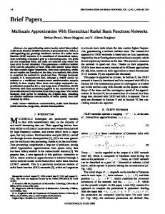
localized basis from the QR factorization of the sparse matrix T , as oppose to the global basis from the eigendecomposition of T , would lead to better approximation accuracy when we numerically implement the Galerkin method in (2.3). When MQ is sufficiently large, M E can even be set to 0 since the QR decomposition of the middle portion of T has generated basis with large enough supports over the attractor of the dynamical system (See Figure 1 (bottom)). In extremely large-scale problems when MQ ¿ N , it is necessary to use a few eigenvectors to stabilize the diffusion forecasting. To illustrate the basis functions constructed by Algorithm 1, let us take the example when the intrinsic manifold M is a unit circle and the observation data are uniformly sampled on M with N =1000. In this case, the eigenfunctions of T are simply the Fourier modes as visualized in Figure 1 (top). Algorithm 1 is applied with M E =20 and MQ = 380 to construct 400 basis functions. As shown in Figure 1 (middle and bottom), the supports of the basis functions from mixed modes gradually grow from a local regime to the whole domain; the basis function oscillates within its supports behaving like a windowed Fourier mode. Hence, applying the basis functions from Algorithm 1 to the Galerkin method in Equation (2.3) is essentially performing a multiresolution analysis on the density p. When p contains local events, the basis functions from Algorithm 1 can capture these features better than the eigenfunctions of T that are all global. Therefore, in the case of local events, the basis functions from Algorithm 1 would lead to better forecasting accuracy. Given M sufficiently large, the error in the approximation in (2.8) is bounded above by: p | A˜ k j − A k j |≤−λk b 0 τ+O (τ), (3.13) where b 0 ≥kb(x)k is an upper bound of the diffusion tensor b(x) in (1.1), λk ≤0 is the kth eigenvalue of the operator Lˆ with the following order, 0=λ0 ≥λ1 ≥.... Note that λk ≤0 ⊥ is also a minimizer of the Dirichlet norm, k∇ f kp eq for any f ∈ H 2 (M ,p eq )∩H k−1 , where H k−1 denotes the eigen subspace spanned by the first k −1 leading eigenfunctions of the operator Lˆ (see the Appendix of [3] or Chapter 6 of [16] for the detailed derivations). With the new proposed orthogonal basis, this error bound still holds with a larger positive constant replacing −λk ≥0 for stochastic problem. In the case of stochastic systems (i.e., b 0 6= 0), numerical examples show that the forecast skill with the new basis functions will not be superior compared to using a large set of eigenfunctions when they are available. However, using the new basis functions to augment existing few eigen functions can improve the forecasting results. For the deterministic problem, the first term in the right hand side of (3.13) vanishes since b 0 =0. Therefore, the error bound is on the order of τ with any orthogonal basis functions including the newly proposed basis. In the numerical section, we will demonstrate that the forecasting skill based on the new basis functions is superior compared to that using the same number of eigenbasis. 8

modes

400

0.01

300

0.005

200

0

100

-0.005 -0.01

0

1

2

3

4

5

6

θ

Figure 1: Top: first 100 leading eigenfunctions as a function of the intrinsic variable θ on periodic domain M =[0,2π). Middle: 400 basis functions by Algorithm 1 with M E =20 and MQ =380. Bottom: the same basis functions as in the middle panel. The color scale is set to [−0.01,0.01] for the purpuse of better visualization. The sizes of the supports of the basis functions grow gradually. The basis funcion oscillates and behaves like a windowed Fourier mode.

9

4 Forecasting dynamical systems In this section, we demonstrate the proposed skill of the diffusion forecasting model in predicting deterministically chaotic and stochastic dynamical systems. In particular, we will consider three examples: a three-dimensional Lorenz model [20], a six-dimensional Lorenz-96 model [21], and a triad stochastic model that is a canonical model for turbulent dynamics [22]. In the deterministic examples, we will see significant forecast improvements using the new basis functions obtained from the QR decomposition relative to the one that uses purely eigenfunctions. For the stochastic example, similar improvement is found relative to the forecasts using a small set of purely eigenfunctions. A crucial component for skillful forecasting of chaotic dynamical systems is the accuracy of the initial conditions. For the diffusion forecasting model in (2.4), we need to specify the coefficients: c k (0)=〈p 0 ,ϕk 〉, which is the representation of the initial density p 0 in the coordinate basis ϕk (x). Practically, however, the initial density, p 0 (x), is rarely known. Instead, one usually needs to specify the initial density from some observations y of the current state. Mathematically, one would like to estimate the conditional density p(x|y) and use it as an initial condition for the diffusion forecasting model. In the remainder of this section, we will first discuss two different methods to specify the initial densities. One of them is the Bayesian inversion introduced in [4] for noisy observations with known error distribution. The second one is a new algorithm based on an application of the Nyström extension [23] for clean data set. Subsequently, we discuss the experimental design. We close this section with the numerical results on the three test examples.

4.1 Specifying initial conditions First, let’s review the Bayesian inversion technique introduced in [4]. Given noisy observations, y n = x n +η n ,

n =1,...,NV ,

with known error distribution, one can specify the initial density by iterating the following predictor-corrector steps: p(x n ) = e τL p(x n−1 |y n−1 ) ∗

p(x n |y n ) ∝ p(x n )p(y n |x n ).

10

(4.14) (4.15)

In (4.14), the prior density, p(x n ), at time n is obtained by solving the diffusion forecasting model in (2.3)-(2.4) starting from the posterior density at the previous time step p(x n−1 |y n−1 ), where the time lag is defined as τ= t n −t n−1 . The Bayes’ theorem in (4.15) is used to specify the posterior density p(x n |y n ). Since the observation error distribution is known, the likelihood function in (4.15) is specified as follows p(y n |x n )= p(y n −x n )= p(η n ). In our implementation, we will start this iterative process with a uniform prior p 1 (x) and discard the posterior densities at first 10 steps to allow for a spin-up time. In the Lorenz-63 and the stochastic triad examples below, we will apply this Bayesian inversion with a Gaussian distributed observation error. When the distribution is not known, one can still implement the Bayes’ correction in (4.15) with a non-parametric likelihood function estimator as proposed in [7]. When the observations are noise-less, then the initial density is given by p(x n |y n )= δ(x n − y n ), such that the coefficients, Z δ(x − y n )ϕk (x)dV (x)=ϕk (y n ). (4.16) c k (t n )=〈p(·|y n ),ϕk 〉= M

Practically, this requires one to evaluate ϕk on a new data point y n that does not belong to the training data set, {x i }i =1,...,N . One way to do this evaluation is with the Nyström extension [23], which is based on the basic theory of reproducing kernel Hilbert space (RKHS) [2]. In our particular application, let L 2 (M ,p eq ) be a RKHS with a symmetric positive kernel Tˆ :M ×M → R that is defined such that the components of (3.11) are given by Tˆi j = Tˆ (x i ,x j ), for training data {x i }i =1,...,N . To be consistent with the conjugation in (3.10), we also define a kernel function T :M ×M → R such that the component of the non-symmetric matrix in (3.12) is given as Ti j =T (x i ,x j )= qˆ −1/2 (x i )Tˆ (x i ,x j )qˆ 1/2 (x j ), P 2 ˆ ˆ i )= N1 N where q(x j =1 K ² (x i ,x j ). Then for any function f ∈L (M ,p eq ), the Moore-Aronszajn theorem states that one can evaluate f at a ∈M with the following inner product, f (a)= 〈 f , Tˆ (a,·)〉peq . In our application, this amounts to evaluating, ϕk (y n ) = qˆ −1/2 (y n )u k (y n ) = qˆ −1/2 (y n )〈u k , Tˆ (y n ,·)〉peq ≈ qˆ −1/2 (y n )

N 1 X Tˆ (y n ,x i )u k (x i ) N i =1

= qˆ −1/2 (y n )

N 1 X Tˆ (y n ,x i )qˆ 1/2 (x i )ϕk (x i ) N i =1

=

N 1 X T (y n ,x i )ϕk (x i ). N i =1

(4.17)

In (4.17), we have used the fact that u j (x i ) is the i j −th component of the matrix U consisting of the eigenvectors of Tˆ in (3.11), i.e. Tˆ U =U Λ; and the fact that the eigenvectors 11

of T are defined via the conjugation formula ϕk (x i )= qˆ −1/2 (x i )u k (x i ). In summary, the estimation of the coefficients in (4.16) requires the construction of an N -dimensional vector whose i th component is T (y n ,x i ) as in constructing the components of (3.12). We will implement this extension formulation on the Lorenz-96 example as well as on the MJO modes application below.

4.2 Experimental design In our numerical experiment below, we consider training the diffusion forecasting model using a data set of length N , {x i }i =1,...,N , where x i := x(t i ) are the solutions of the system of differential equations with a uniform time difference τ= t i = t i −1 . We will verify the forecasting on a separate data set {x n }n=1,...,NV , where x n ∉{x i }i =1,...,N and the time difference is exactly the same as that in the training data set, that is, τ= t n −t n−1 . To specify initial conditions, we define observations, y n = x n +η n , with two configurations. For the Lorenz-63 and the triad examples below, we let the observation noises be Gaussian with variances 1 and 0.25, respectively. For the Lorenz96 example, we let the observations be noise-less, i.e., η n =0. As noted in Section 3, the diffusion forecasting model in (2.5) will be generated using M = M E +MQ modes, where M E denotes the number of eigenvectors and MQ denotes the number of columns of T that are used as specified in Algorithm 1. MQ =0 means that only eigenvectors are used as basis functions. On the other hand, the experiments with modes coming from only the columns of T will be denoted with M E =0. The experiments with the mixed modes are denoted by nonzero M E and MQ . To measure the forecasting skill, we compute the root-mean-square-error (RMSE) of the mean estimate as a function of forecast lead time j τ, E ( j τ)=

³

´1/2 NV X 1 (E[x n+ j ]−x(t n+ j ))2 , NV −10 n=11

(4.18)

R ∗ where E[x n+ j ]= M xe j τL p(x|y n )dV (x) is the mean forecast statistics computed using the diffusion forecasting model. In (4.18), the error is averaged over the verification period, ignoring the first 10 steps to allow for a spin up time in specifying the initial conditions. As a reference, we also show the ensemble forecasting (or Monte Carlo) skill when the underlying model is known. In all of our simulations below, we will use an ensemble of size 1000. To specify the initial conditions, we use the Ensemble Transform Kalman Filter [8, 18] when the observation noises are Gaussian. When the observations are noise-less, we just specify the initial ensemble by corrupting x n with Gaussian noises with variance

12

0.04. With such a small perturbation, we hope to depict the sensitivity of the deterministic dynamical system to initial conditions. In this case, the forecasting statistics are (k) computed by averaging over the ensemble of solutions, {x n+ } . j k=1,...,1000 To quantify the forecast uncertainty, we compare the time evolution of the uncentered second order moment from the diffusion forecasting model and that from the ensemble forecasting using the following RMSE metric, E 2 ( j τ)=

³

´1/2 NV X 1 2 2 2 (E[x n+ , j ]−x n+ j ) NV −10 n=11

(4.19)

x 2 e j τL p(x|y n )dV (x) is the uncentered second order moment com1 P1000 (k) 2 2 = 1000 (x n+ j ) is the empiriputed using the diffusion forecasting model and x n+ k=1 j cally estimated ensemble forecast uncentered second order moment. where E[x n+ j ]=

R

∗

M

4.3 Lorenz-63 example In this section, we test the diffusion forecasting method with new basis functions on the famous Lorenz-63 model [20]. The governing equation of the Lorenz-63 model is given as follows, dx = σ(y −x) dt dy = ρx − y −xz dt dz = x y −bz dt

(4.20)

with standard parameters σ=10, b =8/3, and ρ =28. The dynamics of Lorenz-63 has a chaotic attractor with one positive Lyapunov exponent 0.906 that corresponds to a doubling time of 0.78 time units. Both the training and verification data are generated by solving the ODE in (4.20) with RK4 method with ∆t =0.01. In all of the experiments below, we set τ=0.1. In this example, the training data length is N =25,000 and the verification data length is NV =10,000. In Figure 2, we show the RMSEs of the first and second order moment estimates that are computed based on (4.18) and (4.19), respectively. There are mainly two sets of results in Figure 2: one for M = M E +MQ =2000; another one for M =3000. The set for M =2000 shows that: the proposed basis functions by QR decomposition in Algorithm 1 improve the forecasting results relative to those that purely using eigenvectors based on these two metric evaluations; increasing M E when M is fixed does not improve the forecasting results, i.e., merely using the basis functions from the columns of T in Equation (3.12) are sufficient to make a good prediction when MQ is large enough. The comparison of the results when M =2000 and M =3000 shows that increasing MQ can 13

200

9

180 RMSE of the second order moment

10

8 7 RMSE

6 5

ENS FCST ME =200, MQ =0

4

ME =2000, MQ =0 ME =200, MQ =1800

3

ME =200, MQ =2800 ME =400, MQ =1600

2

ME =0, M Q =2000

1 0

2

4 6 lead time (in model time unit)

8

140 120 100

M =200, M =0 E

Q

M =2000, M =0

80

E

Q

M =200, M =1800 E

Q

60

ME =200, MQ =2800

40

ME =400, MQ =1600 M =0, M =2000 E

20

ME =0, M Q =3000

0

160

0

10

Q

ME =0, M Q =3000

0

2

4 6 lead time (in model time unit)

8

10

Figure 2: RMSE of the mean (left) and second-order uncentered moment (right) of the diffusion forecasting with various choices of basis functions on the Lorenz-63 example.

lead time =0 20 0 -20 250 20 20

255

lead265 time =0

260

270

275

280

lead time =0.5

0

0 -20 250

-20 20 250

255

255

260

260

0

265 270 lead time =0.5

275

265 270 lead time =1

280

275

280

20 0

-20 250

255

260

20 0 -20 250

255255

260 260

-20 250

TRUE

265 270 lead time =1 265 265

ME =2000, MQ =0

270

270

275

280

275

275 280 280

ME =200, MQ =1800

Figure 3: Diffusion forecasting mean estimates of the first component compared to the truth at initial time and forecast lead times 0.5 and 1 model time unit.

14

improve the forecasting accuracy. It is worth emphasizing that the proposed basis leads to better forecasting results than the ensemble forecasting method at all times, while the one of purely eigenfunctions is not. In Figure 3, we show the estimates at 300 verification data points on interval [250,280] for the forecasts that use purely eigenvectors M E =2000,MQ =0 and mixed modes M E = 200, MQ =1800 at the initial time and forecast lead-time of 0.5 and 1. Notice that these times are before and beyond the doubling time of the forecast initial errors, respectively. At the initial time (lead time-0), notice that the Bayesian inversion in (4.14)-(4.15) produces very accurate initial conditions. At lead time-0.5, the mixed-mode forecasts are closer to the truth relative to that of the eigenvectors. The differences between the two are more apparent at lead time-1. Different tests with varying training data sizes (from 5,000 to 50,000) have been performed using the same comparison as discussed just above. The same conclusions above can be drawn from these experiments and results are not shown.

4.4 Lorenz-96 example In this section, we show results for the Lorenz-96 model [21]. The governing equation of the Lorenz-96 model is given as follows, dxj dt

=(x j +1 −x j −2 )x j −1 −x j +F,

j =1,...,d ,

(4.21)

where we set d =6 and F =8 in the experiment here. Note that this model is designed to satisfy three basic properties: it has a linear dissipation (the −x j term) that decreases P the total energy defined as E = 21 dj=1 x 2j , an external forcing term F >0 that can increase or decrease the total energy, and a quadratic discrete advection-like term that conserves the total energy. In our numerical experiment below, both the training and verification data are generated by solving the ODE in (4.21) with RK4 method with time step ∆t =0.05 and we set τ=0.05. Here, we show results with training data of length N =100,000 and verification data of length NV =10,000. For this size of data set, the computing time for the basis functions is recorded in Table 1. Notice that the computational cost for the leading eigenvectors is significantly more expensive than that for QR-decomposition of tall matrices. In Figure 4, we show the RMSEs of the first and second order moment estimates that are computed based on (4.18) and (4.19), respectively. Notice that the proposed mixed basis functions improve the forecasting results relative to those purely based on eigenvectors according to these two metric evaluations. We should point out that the results of mixed basis with M E =2000 and M E =3000 are indistinguishable. So we only report the results of mixed basis with M E =2000. Also, the forecasting skill is slightly improved

15

when MQ in the mixed-mode is increased. In Figure 5, we show the estimates at 1000 verification data points on interval [250,300] for the forecasts that use purely eigenvectors (M E =3000,MQ =0) and mixed modes (M E =2000, MQ =28000) at the initial time and forecast lead-time of 0.5 and 1. Notice that these times are beyond the doubling time of the forecast initial errors. At the initial time (lead time-0), the Nystrom extension produces very accurate initial conditions. At lead time-0.5, the mixed-mode forecasts are closer to the truth relative to that of the eigenvectors. The differences between the two are more apparent at lead time-1. Note that similar trends as above are found in the case of shorter training data sets (namely N =50,000 and 25,000). The only difference is that the forecast errors are larger. Hence, these results are not shown in this paper. Based on these findings, our conjecture is that we may need much longer training data to get results closer to the ensemble forecast in this higher dimensional example. Finally, the results with the mixed basis are also indistinguishable from those obtained using purely QR basis functions with the same number of total modes. This finding is similar to the Lorenz-63 example discussed above. Thus, considering that the QR factorization of an N ×MQ matrix with MQ < N is computationally much cheaper than computing the MQ leading eigenvectors of an N ×N matrix (see Table 1 for an example of wall-clock time comparison), generating basis functions for diffusion forecasting by Algorithm 1 using a large enough MQ is better than the standard diffusion forecasting approach by computing eigenvectors. Table 1: The computational cost (in wall clock time) of computing basis functions based on a data set of length N =100,000. Each case is computed in MATLAB using a singlecore processor of Intel Xeon E7-4830 v2 2.2GHz with a 1Tb of RAM. method

modes

wall clock time (in hours)

QR

10,000 modes 20,000 modes 30,000 modes

0.7 2.6 5.5

2000 modes 3000 modes

15.7 21.8

Eig

4.5 Stochastic triad example In this section, we consider an application of the diffusion forecasting method to the following triad model which was introduced in Chapter 2.3 of [22] as a simplified model

16

16

3.5

14

RMSE of the second order moment

4

3

RMSE

2.5 2

ENS FCST M =2000,M =0 E Q M E =3000,MQ =0 M =2000,M =8000 E Q M E =2000,MQ =18000 M =2000,M =28000

1.5 1 0.5 0

0

1

2

3

E

Q

4

5

M E =2000,MQ =0 M E =3000,MQ =0 M E =2000,MQ =8000 M =2000,M =18000 E Q M E =2000,MQ =28000

12

10

8

6

4

2

6

0

1

2

3

4

5

6

lead time (in model time unit)

lead time (in model time unit)

Figure 4: RMSE of the mean (left) and second-order uncentered moment (right) of the diffusion forecasting with various choices of basis functions on the Lorenz-96 example.

lead time =0 15 10

x1

5 0 -5 -10 200

205

210

215

220

225

230

235

240

245

250

230

235

240

245

250

230

235

240

245

250

lead time =0.5 15 10

x1

5 0 -5 -10 200

205

210

215

220

225

lead time =1 15 10

x1

5 0 -5 -10 200

205

210

215 truth

220

225

ME = 3000, MQ = 0

ME = 2000, MQ = 28000

Figure 5: Diffusion forecasting mean estimates of the first component compared to the truth at initial time and forecast lead times 0.5 and 1 model time unit.

17

for geophysical turbulence, dx ˙, =B (x,x)+Lx −d Λx +σΛ1/2W dt

(4.22)

where x ∈ R3 . The term B (x,x) is bilinear, satisfying the Liouville property, d i v x (B (x,x))= 0 and the energy conservation, x > B (x,x)=0. The linear operator L is skew symmetric, x > Lx =0, representing the β-effect of Earth’s curvature. In addition, Λ>0 is a fixed positive-definite matrix and the operator −d Λx models the dissipative mechanism, with ˙ with scalar σ2 >0 a scalar constant d >0. The white noise stochastic forcing term σΛ1/2W represents the interaction of the unresolved scales. In the following numerical test, we consider B (u,u)=(B 1 u 2 u 3 ,B 2 u 1 u 3 ,B 3 u 1 u 2 )> with coefficients chosen to satisfy B 1 +B 2 +B 3 =0. In our numerical experiment below, we set B 1 =.5,B 2 =1,B 3 =−1.5,     1 1/2 1/4 0 1 0     L = −1 0 −1 , Λ= 1/2 1 1/2 , 1/4 1/2 1

0 1 0

and d =1/2, σ=1/5. Here, the truth is generated by Euler-Maruyama discretization with ∆t =0.01. Here, we show results with training data of length N =25,000 and verification data of length NV =10,000 with temporal step τ=0.05. In Figure 6, we show the RMSEs of the first and second order moment estimates that are computed based on (4.18) and (4.19), respectively. First, notice that using purely eigenvectors (M E =1000,MQ =0) produces forecasting skill close to that of the ensemble forecasting in this example. When the number of eigenvectors is small (M E =100 or M E =200), the forecast skills deteriorate. In the case of deterioration, we can improve the forecast by using mixed modes (see the results for M = M E +MQ =7000). On the other hand, the forecast skill using purely MQ =7000 QR modes is not stable. However, forecasting with QR modes can be stabilized by using more MQ ; but even so, the skill is not superior compared to that with purely M E =1000 eigenvectors. The numerical results here confirm the theoretical error estimate in Chapter 6 of [16]. If the number of modes M is large enough, the M -term approximation error in (2.3) is very small; in this case, the dominant term in the forecasting error is the approximation p error of (2.7), the bound of which is −λk b 0 τ+O (τ) given by (3.13) when eigenbasis is used in (2.8) and (2.9) (see Theorem 6.2 in Chapter 6 of [16] for details). Following the same proof as in Theorem 6.2 in Chapter 6 of [16], if another orthonormal basis is used p in (2.8) and (2.9), the forecasting error is dominated by cb 0 τ+O (τ) since the Dirichlet norm of the new basis functions is larger than the minimizer, k∇ϕk kp eq =c ≥−λk . Hence, in the case of a large M , diffusion forecasting with eigenbasis is the optimal choice for 18

stochastic problems. However, if M is small, i.e., only few eigen functions are available, the M -term approximation error in (2.3) is large and becomes the dominant term in the forecasting error. In this case, one can reduce the M -term approximation error with the mixed modes by Algorithm 1 to reduce the final forecasting error.

5 Forecasting the MJO spatial NLSA modes In this section, we consider predicting two spatial modes associated with the boreal winter Madden-Julian Oscillation (MJO). These two spatial modes were obtained by applying the nonlinear Laplacian Spectral Analysis (NLSA) algorithm [15] on the Cloud Archive User Service (CLAUS) version 4.7 multi-satellite infrared brightness temperature and are associated with the MJO modes based on the broad peak of their frequency spectra around 60 days and the spatial pattern that resembles the MJO convective systems around the Indian Ocean western Pacific Sector (see [15] for the detailed analysis). In [10], a four-dimensional parametric stochastic model has been proposed to predict this time series extensively. Here, we mimic the study in [10] with a slightly different configuration. In particular, we will train our model using the NLSA modes from 3-Sep1983 00:00:00 to 15-Mar-2004 18:00:00, with time discretization τ=6 hours, so the total number of training data points is N =30,000. The verification data is the NLSA modes (obtained separately from the training data) from 01-Jul-2006 00:00:00 to 28-Dec-2008 18:00:00, also with time discretization of τ=6 hours and the total number of verification data points is NV =3,647 (both the training and verification data were provided to us by D. Giannakis, who is one of the inventors of the NLSA algorithm). In Figure 7, we show the RMSE of the mean forecast estimates using various basis functions. Notice that the mixed basis with M E =500, MQ =9500 improves the estimates relative to just using purely M E =500 eigenvectors. The forecasting estimates can be further improved by increasing MQ , say M E =500,MQ =19500. However, when we use only purely MQ =20,000 QR basis, the prediction skill is unstable (dashes). This justifies the use of a few eigen modes to stabilize the performance of the QR basis. In terms of RMSE, notice that the result of M E =3000 is better than that of M E =500,MQ =19500; we speculate that this behavior is because the underlying dynamic is stochastic. However, these two sets of basis functions produce similar results for trajectories at specific times (5, 25, and 40 days) as shown in Figure 8). Notice that the forecasting skill for 15 days is quite high and it deteriorates as the lead time increases to 25 and 40 days. It is worth pointing out that in our implementation, it is implicitly assumed that these two spatial modes can be modeled with a two-dimensional autonomous dynamic, as opposed to the approach in [10] that uses a four-dimensional model (using two auxiliary variables to explain possible interaction of unresolved scales with these two modes).

19

2.5

2

RMSE

1.5

1

ENS FCST ME =100, MQ =0 ME =200, MQ =0 ME =1000, M Q =0 ME =0, M Q =7000 ME =100, MQ =6900 ME =200, MQ =6800 ME =1000, M Q =6000

0.5

0

0

0.5

1

1.5

2

time (model unit time) 5.5 ME =100, MQ =0 ME =200, MQ =0 ME =1000, M Q =0 M =0, M =7000 E Q ME =100, MQ =6900

RMSE of the second order moment

5 4.5 4

ME =200, MQ =6800 ME =1000, M Q =6000

3.5 3 2.5 2 1.5 1 0.5

0

0.5

1

1.5

2

time (model unit time)

Figure 6: RMSE of the mean (top) and second-order uncentered moment (bottom) of the diffusion forecasting with various choices of basis functions on the triad example.

20

RMSE

10 0

10 -1 ME =3000, M Q =0 ME =500, MQ =0 ME =500, MQ =9500 ME =500, MQ =19500 ME =0, M Q =20000

10 0

10 1

forecast lead time (in days)

Figure 7: RMSE of the mean forecast of the diffusion forecasting with various choices of basis functions on the MJO example. Nevertheless, the forecasting skill of these nonparametric models are relatively comparable to those of the parametric model in [10], although their testing and verification periods are slightly different. In their paper, they analyzed the skill of their model for different years. While the nonparametric model we proposed here does not give any mean to understand the physics, it is still advantageous to have the nonparametric model as a reference for developing a more physics-based parametric model. Particularly in this example, it can be concluded that the parametric model in [10] is an appropriate model for predicting these two-dimensional MJO modes, since their predictive skill is relatively comparable (or not worse) compared to that of the diffusion forecasting model.

6 Concluding discussion In this paper, we introduced new basis functions for practical implementation of the diffusion forecasting, a nonparametric model that approximates the Fokker-Planck equation of stochastic dynamical systems. The proposed approach can avoid the expensive computation of a large number of leading eigenvectors of a diffusion matrix T of size N ×N , where N denotes the size of the training data set and could be very 21

forecast lag: 15-day

4

MJO1

2 0 -2 -4 07/01/06

01/01/07

07/01/07

01/01/08

07/01/08

12/28/08

07/01/08

12/28/08

07/01/08

12/28/08

forecast lag: 25-day

4

MJO1

2 0 -2 -4 07/01/06

01/01/07

07/01/07

01/01/08

forecast lag: 40-day

4

MJO1

2 0 -2 -4 07/01/06

01/01/07 truth

07/01/07

01/01/08

ME = 3000, MQ = 0

ME = 2000, MQ = 28000

Figure 8: Diffusion forecasting mean estimates of the MJO1 compared to the truth at forecast lead times of 15-days, 25-days, and 40-days.

22

large. The new basis functions are constructed using the truncated unpivoting Householder QR-decomposition of an N ×(M E +MQ ) matrix, which consists of consecutive MQ columns of T and it’s M E leading eigenvectors. Numerically, the QR-decomposition of a N ×(M E +MQ ) matrix is more efficient compared to finding leading M E +MQ eigenvectors of an N ×N matrix. As long as MQ is large enough such that the time series corresponding to the selected columns fill up the attractor of the dynamical system, the new basis functions perform well in diffusion forecasting. Visually, the supports of the new basis functions gradually grow from a local regime to the whole domain; the basis function oscillates within its supports behaving like a windowed Fourier mode. The locality of the leading modes by QR factorization is inherent because of the diagonally banded structure of T . Using the new basis functions for the M -term approximation of the densities in diffusion forecasting is essentially similar to a multiresolution approximation to the densities. The effectiveness of the proposed algorithm has been demonstrated by numerical examples in both deterministically chaotic and stochastic dynamical systems; in the former case, the superiority of the proposed basis functions over purely eigenvectors is significant, while in the latter case forecasting accuracy is improved relative to using a purely small number of eigenvectors. These numerical results also agree with the theoretical analysis in [3] and [16]. These findings suggest that these new basis functions can be useful for large-scale problems when only a few leading eigenfunctions can be estimated accurately. Acknowledgments. The research of J.H. is partially supported by the Office of Naval Research Grants N00014-16-1-2888 and the National Science Foundation grant DMS1317919, DMS-1619661. We thank D.Giannakis for providing the NLSA modes for the experiments in Section 5. H.Y. is supported by the startup package of the Department of Mathematics, National University of Singapore.

References [1] E. Anderson, Z. Bai, C. Bischof, L. S. Blackford, J. Demmel, Jack J. Dongarra, J. Du Croz, S. Hammarling, A. Greenbaum, A. McKenney, and D. Sorensen, Lapack users’ guide (third ed.), Society for Industrial and Applied Mathematics, Philadelphia, PA, USA, 1999. [2] Nachman Aronszajn, Theory of reproducing kernels, Transactions of the American mathematical society 68 (1950), no. 3, 337–404. [3] T. Berry, D. Giannakis, and J. Harlim, Nonparametric forecasting of low-dimensional dynamical systems, Phys. Rev. E 91 (2015), 032915. [4] T. Berry and J. Harlim, Forecasting turbulent modes with nonparametric diffusion models: Learning from noisy data, Physica D 320 (2016), no. 57-76. [5] T. Berry and J. Harlim, Semiparametric modeling: Correcting low-dimensional model error in parametric models, J. Comput. Phys. 308 (2016), 305–321.

23

[6] T. Berry and J. Harlim, Variable bandwidth diffusion kernels, Appl. Comput. Harmon. Anal. 40 (2016), 68–96. [7] Tyrus Berry and John Harlim, Correcting biased observation model error in data assimilation, Monthly Weather Review 145 (2017), no. 7, 2833–2853. [8] C.H. Bishop, B. Etherton, and S.J. Majumdar, Adaptive sampling with the ensemble transform Kalman filter part I: the theoretical aspects, Monthly Weather Review 129 (2001), 420–436. [9] Frank Böttcher, Joachim Peinke, David Kleinhans, Rudolf Friedrich, Pedro G. Lind, and Maria Haase, Reconstruction of complex dynamical systems affected by strong measurement noise, Phys. Rev. Lett. 97 (2006Sep), 090603. [10] N. Chen, A. J. Majda, and D. Giannakis, Predicting the cloud patterns of the madden-julian oscillation through a low-order nonlinear stochastic model, Geophysical Research Letters 41 (2014), no. 15, 5612– 5619. [11] R. Coifman and S. Lafon, Diffusion maps, Appl. Comput. Harmon. Anal. 21 (2006), 5–30. [12] J. J. Dongarra, Jeremy Du Croz, Sven Hammarling, and I. S. Duff, A set of level 3 basic linear algebra subprograms, ACM Trans. Math. Softw. 16 (March 1990), no. 1, 1–17. [13] M. Ehrendorfer, The liouville equation and its potential usefulness for the prediction of forecast skill. part i: Theory, Mon. Wea. Rev. 122 (1994), no. 4, 703–713. [14] R. Friedrich and J. Peinke, Description of a turbulent cascade by a fokker-planck equation, Phys. Rev. Lett. 78 (1997Feb), 863–866. [15] D. Giannakis, W. w. Tung, and A. J. Majda, Hierarchical structure of the madden-julian oscillation in infrared brightness temperature revealed through nonlinear laplacian spectral analysis, 2012 conference on intelligent data understanding, 2012Oct, pp. 55–62. [16] J. Harlim, An introduction to data-driven methods for stochastic modeling of dynamical systems, Springer (to appear). [17] E.P. Holland, J.F. Burrow, C. Dytham, and J.N. Aegerter, Modelling with uncertainty: Introducing a probabilistic framework to predict animal population dynamics, Ecol. Model. 220 (2009), no. 9–10, 1203 – 1217. [18] B.R. Hunt, E.J. Kostelich, and I. Szunyogh, Efficient data assimilation for spatiotemporal chaos: a local ensemble transform Kalman filter, Physica D 230 (2007), 112–126. [19] C.E. Leith, Theoretical skill of monte carlo forecasts, Mon. Wea. Rev. 102 (1974), no. 6, 409–418. [20] E. N. Lorenz, Deterministic nonperiodic flow, J. Atmos. Sci. 20 (1963), no. 2, 130–141. [21] E.N. Lorenz, Predictability - a problem partly solved, Proceedings on predictability, held at ecmwf on 4-8 september 1995, 1996, pp. 1–18. [22] A.J. Majda, Introduction to turbulent dynamical systems in complex systems, Springer, 2016. [23] Evert J Nyström, Über die praktische auflösung von integralgleichungen mit anwendungen auf randwertaufgaben, Acta Mathematica 54 (1930), no. 1, 185–204. [24] B. Øksendal, Stochastic Differential Equations: An Introduction with Applications, Universitext, Springer, 2003. [25] Jack Poulson, Bryan Marker, Robert A. van de Geijn, Jeff R. Hammond, and Nichols A. Romero, Elemental: A new framework for distributed memory dense matrix computations, ACM Trans. Math. Softw. 39 (February 2013), no. 2, 13:1–13:24. [26] Z. Toth and E. Kalnay, Ensemble forecasting at ncep and the breeding method, Mon. Wea. Rev. 125 (1997), no. 12, 3297–3319.

24