IEEE TRANSACTIONS ON MEDICAL IMAGING
1
Diffusion Basis Functions Decomposition for Estimating White Matter Intra-voxel Fiber Geometry Alonso Ramirez-Manzanares, Mariano Rivera, Baba C. Vemuri, Fellow, IEEE, Paul Carney and Thomas Mareci
Abstract— In this paper, we present a new formulation for recovering the fiber tract geometry within a voxel from diffusion weighted MRI data, in the presence of single or multiple neuronal fibers. To this end, we define a discrete set of Diffusion Basis Functions. The intra-voxel information is recovered at voxels containing fiber crossings or bifurcations via the use of a linear combination of the above mentioned base functions. Then, the parametric representation of the intra-voxel fiber geometry is a discrete mixture of Gaussians. Our synthetic experiments depict several advantages by using this discrete schema: the approach uses a small number of diffusion weighted images (23) and relatively small b values (1250 s/mm2 ), i.e., the intra-voxel information can be inferred at a fraction of the acquisition time required for datasets involving a large number of diffusion gradient orientations. Moreover our method is robust in the presence of more than 2 fibers within a voxel, improving the stateof-the-art of such parametric models. We present two algorithmic solutions to our formulation: by solving a linear program or by minimizing a quadratic cost function (both with non-negativity constraints). Such minimizations are efficiently achieved with standard iterative deterministic algorithms. Finally, we present results of applying the algorithms to synthetic as well as real data. Index Terms— DW-MRI, HARDI, Diffusion basis functions, Axon fiber pathways, Intra–voxel, Basis Pursuit.
I. I NTRODUCTION
W
ATER diffusion estimation has been used extensively in recent years as an indirect way to infer axon fiber pathways and this in turn has made the estimation of fiber connectivity patterns in vivo; one of the most challenging goals in neuroimaging. For this purpose, a special Magnetic Resonance Imaging (MRI) technique named Diffusion Weighted MRI (DW-MRI) is used. This imaging technique allows one to estimate the preferred orientation of the water diffusion in the brain which, in the white matter case, is usually constrained Manuscript received June 17, 2006. This research was supported in part by CONACYT–Mexico (grant 46270) and NIH grants NS42075 & EB007082 to BCV. A. Ramirez-Manzanares was also supported by PhD Scholarship from CONACYT–Mexico. A. Ramirez is with the Computer Science Dept., Centro de Investigacion en Matematicas A.C., Apdo. Postal 402, Guanajuato, Gto., 36000, Mexico. (telephone: (52) 473 73 271 55,
[email protected]). M. Rivera is with the Computer Science Dept., Centro de Investigacion en Matematicas A.C., Apdo. Postal 402, Guanajuato, Gto., 36000, Mexico. (telephone: (52) 473 73 271 55,
[email protected]). B.C. Vemuri is with Dept. of Computer Information Science and Engineering, University of Florida, Gainesville, Fl. 32611, USA. (
[email protected]), P. Carney is with the Dept. of Pediatrics, University of Florida, Gainesville, Fl. 32610, USA (
[email protected]) T. Mareci is with Dept. of Biochemistry & Molecular Biology, University of Florida, Gainesville, Fl. 32610, USA. (
[email protected]).
along the axon orientations. This information is very useful in neuroscience research due to the changes that occur in the neural connectivity patterns with neurological disorders and, in general, with brain development [1], [2]. The water diffusion angular variation has been summarized, in most medical applications, by Diffusion Tensor Magnetic Resonance Images (DT–MRI) [3], [4]. In [5], Stejskal-Tanner presented a mono-exponential model of the decayed MR signal. Afterwards Basser et al. [3], developed the DT model: S(qk , τ ) = S0 exp(−qTk Dqk τ ) + εk ,
(1)
where the anisotropic diffusion coefficients are summarized by the (3 × 3) symmetric positive definite tensor D, S0 is the measured signal in the absent of a diffusion magnetic field gradient (a standard T 2 image [1]), the attenuation factor on the observed DW–MR signal S(qk , τ ) is determined by the gradient diffusion vector qk , the tensor D and the effective diffusion time τ . The gradient diffusion vector qk = γδGgk , where γ is the gyromagnetic ratio, δ is the duration for which the directional magnetic gradient is applied, G is the magnitude of the applied diffusion magnetic field gradient and T the unit vector gk = [gkx , gky , gkz ]k=1,...,M indicates the k– th orientation of the diffusion–encoding gradients. In model (1), εk represents noise with Rician distribution, see [6] and the Appendix. A standard protocol for indirectly measuring water diffusion consists in acquire M three-dimensional (3D) images along independent orientations gk . A convention is to 2 let b = (γδG) τ and thus making b (denoted in s/mm2 ) a constant directly proportional to the magnitude of the diffusion vectors and the acquisition time. Given S0 and at least six measurements S(qk , τ )k=1,...,6 , the DT is estimated by a Least Squares (LS) procedure [3], [7]. The DT can be visualized as a 3D ellipsoid, with the principal axis aligned with the eigen–vectors, [ˆ e1 , eˆ2 , eˆ3 ], and scaled by the eigen–values, λ1 ≥ λ2 ≥ λ3 . Such eigen–values indicates diffusivity along the eigen–vectors. Thus, eˆ1 is named the Principal Diffusion Direction (PDD) and is associated with the orientation of the fibers in the case of a single fiber bundle within a voxel. Therefore, the partial volume effect limits the capacity of determining the fiber orientations: the observed DT at voxels where two or more fibers cross, split, or merge is the average of the diffusion in the constituent fiber orientations. Thus the DT inadequately represents such an intra-voxel information [8]–[10]. On the other hand, the computation of non-parametric diffusivity coefficients with High Angular Resolution Diffusion
c 2007 IEEE 0000–0000/00$00.00 °
IEEE TRANSACTIONS ON MEDICAL IMAGING
2
Images (HARDI) fails to estimate correctly 2 or more fiber orientations (as the Apparent Diffusion Coefficient (ADC) Map [11]), as is deeply discussed in [11]–[14]. In this work we use the Gaussian Mixture Model (GMM) as a more plausible model for the decayed signal phenomenon [12]:
1
1 2
2
3
3
4
4
5
5
(a) S(qk , τ ) = S0
L X
βj exp(−qTk Dj qk τ ) + εk ;
(2)
j=1
where the real coefficients β ∈ [0, 1] indicate the contribution of the tensor³ Dj (the fiber ´ oriented with Dj ) to the total DW P β = 1 . The GMM explains quite well the signal, i.e., j j diffusion phenomenon for two or more fibers within a voxel under the assumption of no exchange between fibers, i.e., the signals are independently added. The GMM was explored by Basser et al. in [15]; they concluded that its solution requires a large number of measurements S(qk , τ ), and remarked the numerical problems because of the non-linearity. Frank [16] expanded his Spherical Harmonic Decomposition (SHD) method to the N –fiber case by using the model (2). Parker and Alexander [17] used the Levenberg-Marquardt algorithm to fit ¨ the GMM. Recently Ozarslan et al. [14] used the GMM to perform an important refinement in their Diffusion Orientation Transform (DOT) for computing a diffusion displacement probability. See [1] for more details about model in (2). However, in the best of our knowledge, the GMM has not been efficiently fitted to the DW-MR signals. We describe below the better implementations for this aim. Tuch et al. [12], [13], proposed a non–linear LS method for solving (2). That approach fixed the eigen–values for the diffusion tensors and solves the GMM for the number of tensors, L, the coefficients, β, and the tensor’s orientation angles. The drawbacks of the method are: the large number of required diffusion images {S} that notably increases the acquisition time (for instance, 126 diffusion 3D–images are used in [12], [13] and more recently 54 measurements in [17]) and the algorithmic problems related to the non-linearity of (2). Thus, multiple restarts of the optimization method are required for preventing the algorithm from settling in a local minimum. Note that it is necessary to choose between fit a single Gaussian or a GMM, or to fit both and then choose the one which explains better the DW-MR signals. Furthermore, no stable solution has been reported for more than 2 fiber bundles, i.e. for L > 2 (see [12] and [13, Chap. 7]). Another interesting model–based approach is reported in [18], by assuming that the observed diffusion signal results from the hindered (extra–axonal space) and the restricted (intra axonal space) water diffusion. Although such a model was extended to a multi-fiber case, the above explained model– selection problem is present. Q–space method is an alternative non-parametric representation. This method is based on the Diffusion Spectrum Imaging (DSI) [19]–[21], by exploiting the Fourier Transform (FT) relationship from which an Ensemble Average Probability (EAP) is computed. The EAP [13], [22] is defined as
(b)
Fig. 1. 2D Schema of DBFs. (a) Continuous-blue line shows the DBFs generated by an uniformly distributed tensor basis with cardinality N = 5; the doted-red line shows the signal S(q) generated by an arbitrary DT. (b) Schema for a two fiber case, the dotted-red line shows the S(q, τ ) measured signals for the two arbitrary tensors, the half-addition of both signals are shown in the cross-marked black line. See text for details.
P (r) = S0−1
Z
T
S(q, τ )e−iq r dq = F −1 [E(q, τ )] ,
(3)
where the displacement vector r = re − r0 defines the particle displacement (located at r0 at the beginning and at re at the end of the experiment), F −1 denotes the inverse FT with respect to the diffusion vector q, and E(q, τ ) = S(q, τ )/S0 . The non-parametric DSI can represent several fibers within the voxel, although the large number of required DW images makes the method impractical for medical purposes. Recent methods for recovering EAP, as Q–Ball [23] , Persistent Angular Structure (PAS) [24] or DOT [14] have demonstrated good results with a smaller number of diffusion images; for instance, in [24] are used 54 measurements. However it is desirable to diminish this number for practical purposes. A drawback in the previous methods is that, for estimating the intra–fiber orientations, the maxima of the EAP need be computed as a postprocessing [13], [14], [22], [23]. Recently, spherical–deconvolution techniques explain DW– MR signals as the convolution of a single fiber response with the Fiber Orientation Distribution (FOD). FOD is represented with a linear basis for spherical functions in [25], [26] and in [27] was proposed a maximum-entropy formulation of the spherical deconvolution (MESD) problem with a non– linear deconvolution kernel (a generalization of PAS method). Although [27] presented better results, the method does not guarantee the attainment of the global minimum and requires a significant computational effort. In [28] it is proposed a simple axial symmetric model of diffusion, where the angular distribution of fibers is computed by a deconvolution process and by assuming constant, both, mean diffusivity and perpendicular diffusivity in all the white matter (a similar assumption was used in [26]). In most previous works [12], [14], [23], [25], [26], [28], large b-values (larger than 2000 s/mm2 ) or large datasets are required for recovering good angular resolution, which is somewhat impractical in a clinical setting. In a recent article [10], a regularization-based approach was proposed for recovering the underlying fiber geometry within a voxel. That approach reconstructs the observed tensors as a linear combination of a given tensor basis. However the multitensor model is computed from previously fitted DTs (instead of the raw measurements S(qk , τ )) and thereby important
IEEE TRANSACTIONS ON MEDICAL IMAGING
3
with αj ≥ 0; where we define the j–th DBF by: ¯ j qk τ ), φj (qk , τ ) = S0 exp(qTk T
¯j Fig. 2. Normalized diffusion weighted signal E(q) for a base Tensor T and its corresponding EAP. The black axis denotes the PDD.
information is lost. In this paper, a novel method for reconstructing the intra– voxel information is presented. We note that present work extends previos conference papers [29], [30]. The method is based on the solution of a discrete version of the parametric model in (2). Synthetic experiments for a realistic situation demonstrate the advantages of our method: the intra-voxel information for more than 2 axon fibers can be inferred at a fraction of the acquisition time with respect to methods that require a larger set of DW-MR images (M ≥ 54) or large b values (b ≥ 2000 s/mm2 ). We present two variants of our method: one based on the minimization of a Linear Programming (LP) problem (which is computationally more efficient) and another based on the minimization of a regularized quadratic cost function (which improves the quality of the results for noise corrupted data), both with non-negativity constraints. II. T HE D IFFUSION BASIS F UNCTIONS In this section we propose a discrete diffusion model based on the GMM in (2). In order to simplify the solution of such a model, we propose to use a set of Diffusion Basis Functions (DBF) {φ}, which are generated from a tensorial basis as the one used in [10]. Such a tensor basis is defined ¯ with cardinality equal to N . as a fixed set of tensors T ¯ j are chosen, such that, they The individual base tensors T are distributed as uniform as possible in the 3D space of orientations, and their anisotropy is chosen according to prior information about longitudinal and transversal fiber diffusion. For the human brain, it is reasonable to assume that the anisotropy and magnitude of the water diffusion for a single fiber in white matter is almost constant in all the volume [12], [26], [28], we will discuss this topic in section VIII. For instance, one could expect that longitudinal fiber diffusion is about five times than the transversal one: [λ1 , λ2 , λ3 ] ≈ [1×10⁻³ mm2 /s, 2×10⁻⁴ mm2 /s, 2×10⁻⁴ mm2 /s] [1], [13]. However, these values could change between patients, so that, we instead recommend setting the basis eigen–values according to the procedure described in section IV-A.2. By fixing the basis eigen–values, we reduce the degrees of freedom for the problem. Thus, we propose to model the DW–MR signal, at each voxel, with: S(qk , τ ) =
XN
j=1
αj φj (qk , τ ) + ηqk + εk ;
(4)
(5)
where, φj (qk , τ ) is understood as the coefficient of the diffusion weighted signal for the diffusion vector qk due to a single ¯ j . The non-negative αj fiber modelled by the base tensor T denotes the contribution of the j–th DBF {φj (qk , τ )}k=1,...,M . Note that the basis {φ} is incomplete, because the available orientations are a discretization of the 3D space (see section VIII). So that, a residual ηqk in the signal representation is observed. By choosing a basis with a large cardinality we can diminish ηqk , until it becomes insignificant enough, and then neglected for practical purposes. As can be noted, an advantage in our model (4) is that the unknowns are the α–coefficients and the φj (qk , τ ) coefficients can be precomputed. In fact, we need to compute the best linear combination of DBFs that reproduce the signal S. This is illustrated in the 2D schema shown in Fig. 1. Panel 1(a) shows a single fiber case where we compute the αj values that, given a set of 5 DBFs (continuous-blue lines) reproduce the S(qk , τ )k=1,...,M measurements (dotted-red line) as accurately as possible; for this particular case, we expect α3 ≈ 1. On the other hand, for the two fiber case (Panel 1(b)), the α coefficients should reproduce the addition (plus-sign black line); in this case, we expect α3 ≈ α5 ≈ 0.5. Note that in our approach, we do not work with the schematized continuous measurements in Fig. 1, but with a discrete set of M samples (measurements). Although in this work we use the free–diffusion model in (5) for setting the DBF, it is possible to use another diffusion model as the cylinder restricted diffusion model proposed in [31], see discussion in section VIII. By substituting our observation model (4) in the EAP in (3), we obtain: P (r) = S0−1
N X
αj F −1 [φj (q, τ )] .
(6)
j=1
As the DBF is a Gaussian (according to the free–diffusion model) and the FT of a Gaussian results in a Gaussian ¡ ¢ F[g((x), Σ)](w) ∝ g(w, Σ−1 ) , then in our case, the EAP is a GMM with peaks oriented along the PDDs of the corresponding base tensors. Moreover, the peaks in P (r) are determined by the largest αj and therefore also the fiber orientations. This is illustrated in Fig. 2 where we show for a given base tensor the synthetic DW signal and the EAP computed with (3). As can be seen, the maxima of a single EAP in the GMM corresponds with the PDD of the associated base tensor. III. N UMERICAL S OLUTIONS F OR DBF M ODEL In this section we present two procedures for estimating the coefficients α in (4). We first introduce the notation that will be useful in the following. The observation model (4) can be written in matrix form as S = Φα + η;
(7)
IEEE TRANSACTIONS ON MEDICAL IMAGING
4
with αj ≥ 0, ∀j; Φ is an M ×N matrix where the j–th column corresponds to the j–th DBF (Φj = [φj (qk , τ )]k=1,...,M ) and S ∈ ℜM is the vector composed by all the DW signals. Note that because of our requirements, the matrix Φ is rectangular: we want to acquire as few as possible S signals and to recover solutions with a high angular resolution; for instance we use N = 129 DBFs and M = 23 DW-MR images. Consequently, we have more unknowns, α’s, than data, S’s; the problem (7) is ill-posed and should be constrained or regularized in order to compute a meaningful solution. In the following subsections we introduce two algorithms for computing the best α vector by means of introducing prior information about desired features in the solution.
A. Basis Pursuit Algorithm Compact signal representation is a well studied problem by signal processing researchers [32]–[34]. In that context, it is convenient to represent a given signal by a set of coefficients associated with elements of a dictionary (or base) of functions. The elements of such a dictionary are called atoms (or basis functions). The idea is to select from the dictionary the atom decomposition that best match the signal structure, using a criterion for choosing among equivalent decompositions. A commonly used criterion is the basic principle of sparsity, i.e., to represent the signal with the fewest atoms as possible. Additionally, a desirable feature is to achieve the decomposition in a computationally efficient way. In our notation, Eq. (7) is the mathematical model for representing the decomposition of the signal S ∈ ℜM as a linear combination of atoms Φj in a dictionary Φ. In [32], the Basis Pursuit (BP) technique was proposed for solving the problem (7), i.e., for computing the α coefficients. Based on the BP framework, we propose to compute a solution to (7) by means of an LP problem of the form: P min kαk1 = j αj = eˆT α subject to Φα = S, αj ≥ 0 , ∀j,
(8)
where eˆ is a vector with all its components equal to one (we can use just eˆT α instead of kαk1 since the sign of the components of α is already constrained). Because of the noise and given that Φ is an uncomplete dictionary, the signal reconstruction constraint in (8) could not to be fully accomplished, resulting in an over-constrained LP problem. Therefore an appropriate minimization procedure is required: an interiorpoint method which tries to minimize the magnitude of the residual vector ηα = Φα−S (see [35]). In our experiments we used the powerful primal-dual predictor-corrector algorithm by Merhotra (see [35], [36]) that computes the results in a fraction of the computational effort required by other less-sophisticated interior point methods. The BP method have shown, in general, a better performance with respect to other pursuit techniques as, for instance, Matching Pursuit (MP) [34]. The BP method represents with few α coefficients the atoms that best fit the local structures.
B. Spatial and Coefficient-Contrast Regularization The adverse effect of noise or a limited number of measurements S(qk , τ ) could possibly lead most methods to miss the original fiber directions. In such situations, the BP method could erroneously estimate the α coefficients: they may do not correspond to the correct axonal fiber orientations or may not indicate the right number of fibers in each voxel. In such a case, the use of a spatial regularization diminishes the noxious noise effect [37], [38]. In this work, in order to reduce such an adverse effect, we propose to filter the α coefficients and therefore to introduce prior knowledge about the piecewise smoothness assumption on the axon fibers orientation and for promoting high contrast in the α–coefficients. In our notation, a voxel position is denoted by r = [x, y, z], such that αjr is the αj –th coefficient at the r voxel position and Nr denotes the second order spatial neighborhood of r: Nr = {s : |r − s| < 2}. Therefore the αjr coefficient is implicitly associated with the fraction diffusion in a given ori¯ j ), entation (i.e. along the PDD of the associated base tensor T and the spatial smoothness of the αj layer (∀r) is intimately related with the fiber’s spatial smoothness. Moreover, if an axon bundle have a trajectory close parallel to the j-th PDD, then we expect a large value for the αj coefficient. Thus, by smoothness, the neighbor voxels along the orientation of the fiber should have its αj coefficient large too. Similarly, such a behavior is expected for the close-to-zero coefficients too: if a fiber is not present in a position, then it is not likely to detect its prolongation along its orientation. The above prior knowledge is coded in the regularization term [10]: X X 2 wjrs (αjr − αjs ) ; Us (α, r) = s:s∈Nr
j
which penalizes the difference between neighboring coefficients along the underlying fiber orientations. Such a process is controlled with the anisotropic weight factors wjrs = T ¯ 4 (s − r) T j (s − r) / ks − rk . Additionally, we promote high contrast in the α–coefficients to distinguish the representative α–coefficients (orientations) from the noisy ones and to compute a sparse solution. Thus we force each αjr coefficient to be different from the arithP metic mean α ¯r = α /N , by minimizing Uc (α, r) = jr j P 2 − j (αjr − α ¯ r ) , see [10]. Finally, the cost function that we propose to minimize is: 2
U (α, r) = kS − Φαr k2 + µs Us (α, r) + µc Uc (α, r) ,
(9)
subject to αjr ≥ 0, where the non–negative control parameters µs and µc allow us to tune the amount of regularization. The potentials were chosen in order to keep the cost function (9) quadratic. Thus by equaling to zero the partial derivative with respect to each αjr results in a constrained linear system. It can easily be solved by using a Gauss-Seidel (GS) scheme [39] (used in our experiments because of its efficient use of memory) or a conjugate gradient technique which is time efficient [35]. The non-negativity constraint over the α coefficients is accomplished along with the minimization with a particular case of the well known Gradient Projection: the negative αjr values are projected to zero in each iteration
IEEE TRANSACTIONS ON MEDICAL IMAGING
[35]. The tuning of the spatial regularization parameter is quite simple: the large µs value eliminates noise but a too large value over–smooths the recovered solution. We found that, in our experiments, µs ∈ [0.5, 3.0] produces an adequate noise reduction. As was explained in [10], the µc value is gradually introduced because it is important to perform the coefficient–contrast regularization once we have an intermediate regularized ¡solution: for each¢iteration k = 1, 2, . . . , n, we (k) set µc = µc 1.0 − 0.95100k/n that increases to µc in the approximately 90% of the total number of iterations n, with µc ∈ [0.1, 0.5] for all our experiments.
5
i+1 i
(a)
(b)
Fig. 3. Example of a single fiber case. (a) Discrete solution (cluster) composed with two DBFs. (b) Level curves of kΦα − Sk2 for αi (X-axis) and αi+1 (Y-axis) coefficients, with αk = 0, ∀k 6= i, j. See text for details.
IV. I MPLEMENTATION D ETAILS In this section we describe important implementation details to be taken into account for obtaining high quality results. A. Designing the Tensor Basis There are two main aspects: (i) the eigen–vector orientations and (ii) the eigen–values. 1) Orientations: The basis orientation set depends on a compromise between the desired resolution of the results and the computational effort. The procedure for obtaining the 3D balanced orientations is exactly the same as that of selecting the acquisition DW orientations in the MR machine [40], i.e. one can use the almost uniformly distributed directions given by the n-fold tessellated icosahedron hemispheres, or by using an electrostatic repulsion model [41]. In particular, we used recursive tessellations of a square pyramid (having equilateral triangles as sides) that results in {3, 9, 33, 129, 513, 2049, . . .} almost uniform orientations for {0, 1, 2, 3, 4, 5, . . .} successive tessellations, respectively. We used N = 129 orientations in all our experiments. Note that in our approach, the high angular resolution is in the tensor basis but not in the acquired signals S(q, τ ). 2) Eigen–Values: As was mentioned in section II, we can make use of prior information about longitudinal and transversal diffusion. As the diffusion parameters may change between patients or by scale-factor effects in the signal, then it is important to determine the best set of parameters for each experiment. In present work we perform experiments using rat brain data. The optimal parameters were determined by fitting the standard DT model to the voxels in the corpus callosum, a well known region with high Generalized Anisotropy (GA) [42] and relatively free of crossing fibers. Then, the mean values of the fitted DTs are used for designing the base; in particular we found [λ1 , λ2 , λ3 ] = [6 × 10⁻⁴ mm2 /s, 2 × 2 10−4 mm2 /s, 2 × 10⁻⁴ mm P /s]. We do not constrain j αj = 1 because (assuming that S0 is accurate enough) a well designed basis will automatically satisfy it. A summation different enough from 1 indicates error in the DBF design; in our experiments, for such a voxelwise summation, we obtained a mean value equal to 0.96. B. Computation of a Continuous Solution The formulation presented in section II produces a discrete set of PDDs that can be conveniently post-processed for
obtaining refined continuous orientations with smaller angular errors. Assuming the 2D example shown in Fig. 3, the BP approach gives us a solution with minimum kαk1 and minimum magnitude of the error rα = Φα − S (as shown in the Panel 3(b)), the maximum diffusion orientation (plotted in a dotted-red line), lies at an intermediate value between ¯ i and T ¯ i+1 the orientation of the two closest base tensors T (continuous–lines). For computing the continuous solution we group the orientations in clusters and we assign an unique orientation to each cluster. A cluster Ω = {vl } is a set of vectors associated with the base tensors that contribute to the GMM (their corresponding coefficients are αl > 1 × 10⁻² ) and with a transitive neighborhood relationship. We denote by Nv l
¯ j ) : elj ∈ E} ∪ = {vj = P DD(T ¯ j ) : v T vl ≤ max v T vl } {vj = −P DD(T j
elk ∈E
k
the set of neighbor vectors to vl ; where E is the set of edges ¯ l ) is the first eigenin the tessellation structure and P DD(T ¯ l . The cluster centroid Q ¯ ∈ ℜ3 is vector of the base tensor T then computed by the weighted summation: X ¯= αl vl . (10) Q vl ∈Ω
Therefore we obtain a new GMM with continuous DTs (with ¯ and mixture eigen–values [λ1 , λ2 ,¯λ3¯] and oriented along Q) ¯ ¯. coefficients equal to ¯Q Due to the high sparsity in the α vector for the discrete solutions, the processed clusters were composed in most cases of two or three vectors. C. Avoiding Ill-conditioning in Merhotra’s Algorithm Last iterations of Merhotra’s algorithm could involve to solve an ill-conditioned problem of the form Ax = b, see [35]. For avoiding such a problem, we modify A by adding the value κ = 5×10⁻⁶ to the diagonal when its smallest eigen– value is less than 1 × 10⁻³ : we solve instead (A + κI)x = b. D. Fast Convergence In order to speed up the GS solver for (9), we use the BP solution as the initial guess for α. Then we eliminate noise by means of a spatial integration performed by a small number of iterations of the GS approach.
IEEE TRANSACTIONS ON MEDICAL IMAGING
6
(a) S(qk , τ )
(b) DS 2 coplanar
(c) CS 2 coplanar
(d) DS 3 coplanar
(e) CS 3 coplanar
(f) EAP for (e)
(g) DS 4 coplanar
(h) CS 4 coplanar
(i) DS 4 non-coplanar
(j) CS 4 non-coplanar
(k) DS 5 non-coplanar
(l) CS 5 non-coplanar
Fig. 4. Results of noise-free synthetic experiments. The fiber axis are plotted in black. (a) DW signal for 4 non–coplanar fiber orientations, b=1200 s/mm2 , Dal = 1 × 10⁻³ , Dtr = 2 × 10⁻⁴ . (b) and (c) Discrete Solution (DS) and refined Continuous Solution (CS) for 2 coplanar fibers, b=800 s/mm2 , Dal = 6 × 10⁻⁴ , Dtr = 2 × 10⁻⁴ (these diffusion parameters are similar to those obtained from the rat brain white matter). (d), (e) and (f) DS, CS and EAP for 3 coplanar fibers, b=800 s/mm2 , Dal = 6 × 10⁻⁴ , Dtr = 2 × 10⁻⁴ . (g) and (h) DS and CS for 4 coplanar fibers, b=1350 s/mm2 , Dal = 1 × 10⁻³ , Dtr = 2 × 10⁻⁴ . (i) and (j) DS and CS for 4 non-coplanar fibers, b=1200 s/mm2 , Dal = 1 × 10⁻³ , Dtr = 2 × 10⁻⁴ . (k) and (l) DS and CS for 5 non-coplanar fibers, b=1000 s/mm2 , Dal = 1 × 10⁻³ , Dtr = 2 × 10⁻⁴ .
V. R ESULTS ON S YNTHETIC DATA For showing important features of the signals, all previous figures were generated using b=5000 s/mm2 and a high angular resolution (so that, the S(qk , τ ) signal generates contrasted plots). In real imaging protocols lower values for previos parameters are preferred. In this section, we show synthetic results obtained by using only 23 diffusion encoding orientations, relative small b values and small ratios between the longitudinal diffusion (Dal ) and the transversal diffusion (Dtr ), see Fig. 4. An example of a realistic S(qk , τ ) is shown in Panel 4(a). Same Fig. shows synthetic noise-free experiments and demonstrates the capability of our method for resolving multiple fiber orientations (in yellow parallelepiped) with a small error. We show the discrete solution and the continuous solution computed according to the procedure described in subsection IV-B. The real axis for the maximum diffusion orientations are plotted as black lines. In Panel 4(f) we show, for illustrative aims, the EAP for the recovered multiDT in Panel 4(e), computed with inverse FT of the GMM as indicated in [8]. We note that the peaks of the EAP (aligned, as expected, with the PDDs of the recovered multiDTs) corresponds with the axes for the maximum diffusion orientations. Such EAP peaks are directly determined by the orientation of DBF with significant α values. Thus, in our approach, for bunch fiber detection we look for large α values and the computation of the EAP is not needed. For computing previous solutions, the BP solver requires approximately 35 ms per voxel, implemented in C language, on a modest PC Pentium IV, 2.8Mhz. In order to analyze the expected error in real conditions,
(a) θ¯ = 9.21◦
(b) θ¯ = 7.76◦
(c) θ¯ = 6.98◦
(d) θ¯ = 6.47◦
Fig. 5. Simulated crossing fibers, the signals were corrupted with Rician noise, SNR = 2.0 (6.02 dB). (a) Solution without regularization (BP based method). (b), (c) and (d) noise removal effect with the quadratic formulation ¯ The solution in (d) is over–smoothed because and the mean angular errors θ. of a too large µs value. See text for details.
IEEE TRANSACTIONS ON MEDICAL IMAGING
VI. R ESULTS ON R AT B RAIN DW-MR DATA
TABLE I M EAN ANGULAR ERROR θ¯ V S . SNR. M = 23 MEASUREMENTS , b = 1250 s/mm2 , DBF PARAMETERS [λ1 , λ2,3 , N ] = [9 × 10⁻⁴ , 1 × 10⁻⁴ , 129], [Dal , Dtr ] = [1 × 10⁻³ , 2 × 10⁻⁴ ], COMPARTMENT SIZES βi = 1/3, (i = 1, 2, 3).
DIFFUSION PARAMETERS
SNR
θ¯
2 (6.02 dB)
15.21
4 (12.04 dB)
7.75
6 (15.56 dB)
5.29
8 (18.06 dB)
3.68
10 (20.00 dB)
3.66
12 (21.58 dB)
2.74
14 (22.92 dB)
2.15
16 (24.08 dB)
1.85
TABLE II M EAN ANGULAR ERROR θ¯ V S . BASIS PARAMETERS . N = 129, M = 23 b = 1250 s/mm2 , SN R = 6 (15.56 D B), DIFFUSION PARAMETERS [Dal , Dtr ] = [1 × 10⁻³ , 2 × 10⁻⁴ ],
DIFFUSION MEASUREMENTS ,
COMPARTMENT SIZES
βi = 1/3, (i = 1, 2, 3).
λ2,3
° ° ¯ − DD ,D ° °T tr al
λ1 8.50 ×
10−4
0.5 ×
F
10−4
1.5 ×
θ¯
10−4
5.45
1.0 × 10⁻⁴
5.77
9.00 × 10⁻⁴
1.0 × 10⁻⁴
9.50 × 10⁻⁴
1.5 × 10⁻⁴
5.0 × 10⁻⁵
5.02
1.00 × 10⁻³
2.0 × 10⁻⁴
0.0
5.46
1.05 × 10⁻³
2.5 × 10⁻⁴
5.0 × 10⁻⁵
5.11
10−3
10−4
1.0 × 10⁻⁴
4.96
3.5 × 10⁻⁴
1.5 × 10⁻⁴
5.60
1.10 ×
3.0 ×
1.15 × 10−3
Mean Angular Error vs. SNR and b values 16
b Values 14
Mean Angular Error (degrees)
we performed 3D synthetic experiments simulating 3 noncoplanar fibers within the voxel, oriented with azimuthal and elevation angles equal to [π/4, π/4], [3π/4, π/4] and [3π/2, π/4], respectively. In Tables I, II, III and Fig. 6, we ¯ of 100 experimenshow the computed mean angular error, θ, tal outcomes taking into account 4 important variables that directly affect the solution quality: 1) Noise robustness. The S(q, τ ) signals were corrupted with Rician noise with an SNR (see the Appendix for SNR definition) range from 2 (6.02 dB) to 16 (24.08 dB), see Table I. 2) Error in the diffusion basis with respect to the diffusion parameters in the data. The purpose of this set of experiments is to evaluate the sensitivity of the method to deviations in the pre–fixed DBFs with respect to the real diffusion parameters which change between voxels, see Table II. 3) Method capability for recovering intra–voxel geometry with different b-values, see Fig. 6. 4) Sensitivity to changes in the fibers compartment size, see Table III. ¯ is small enough for As one can see, the mean angular error, θ, a large set of parameter variations. These results improve the methods of the state-of-the-art. The method in [43] is restricted to recover only one or two fibers orientations within a voxel, and reports a mean angular error smaller than 10 degrees for simulated fibers with an SN R=80 (We note that the SN R is not defined in [43], so can not be directly compared with our SNR definition). In our work, we obtained θ¯ ≈ 5 degrees for SNR=6 (15.56 dB), for the 3 fibers case, see Table I. For SNR ≥ 6, our algorithm is capable of yielding high quality results ( θ¯ ≤ 6 degrees) with realistic b values, see Fig. 6. Fig. 5 demonstrate the spatial and contrast regularization performance, introduced in section III-B. We simulate a crossing of two fibers with b=1250 s/mm2 , Dal = 1 × 10⁻³ mm2 /s, Dtr = 2 × 10⁻⁴ mm2 /s, SNR = 2 (6.02 dB) and a 2D tensor basis composed of N = 30 orientations. Panel 5(a) shows the noise corrupted recovered solution with the BP procedure (i.e. without regularization). The resultant orientation errors are similar to the ones reported by Perrin et al. [44], where θ¯ ≈ 30 degrees was reported in a crossing zone for a realistic phantom and, in our opinion, reveals the need of introducing a regularization mechanism for dealing with highly noise data. Panels 5(b),5(c) and 5(d) show the noise removal effect when our proposed quadratic regularized method is used. The regularization parameters used in the experiments were [µs , µc ] = [1.0, 0.5], [µs , µc ] = [2.0, 0.5] and [µs , µc ] = [3.0, 0.5], for in Panels 5(b), 5(c) and 5(d), respectively.
7
− o x + * .
12
750 1000 1250 1500 1750 2250
10
8
6
4
2 2
4
6
8
10
12
14
16
SNR
Under deep anesthesia, a Sprague Dawley rat was transcardially exsanguinated then perfused with a fixative solution of 4% paraformaldehyde in phosphate buffered saline (PBS). The corpse is stored in a refrigerator overnight then the brain was extracted and stored in the fixative solution. For MR measurements, the brain was removed from the fixative
Fig. 6. Mean angular error θ¯ Vs. SNR and b-values. M = 23 diffusion measurements, tensor basis parameters [λ1 , λ2,3 , N ] = [9 × 10⁻⁴ , 1 × 10⁻⁴ , 129], diffusion parameters [Dal , Dtr ] = [1 × 10⁻³ , 2 × 10⁻⁴ ], compartment sizes βi = 1/3, (i = 1, 2, 3). See text for details.
IEEE TRANSACTIONS ON MEDICAL IMAGING
(a) ROI
8
(b) Zoom of(a)
(d) Zoom of(c)
(c) ROI
(e) ROI
(f) GA, FA Maps
Fig. 7. Computed DTs of the GMM from a real rat brain DW-MR set superimposed over the GA axial map. Note several fiber crossings and splits. (f) GA map, FA map and their difference for the ROI in (a).
TABLE III M EAN ANGULAR ERROR θ¯ V S . C OMPARTMENT SIZES ([β1 , β2 , β3 ]). M = 23 DIFFUSION MEASUREMENTS , b = 1250 s/mm2 , SN R = 8 (18.06 D B), TENSOR BASIS PARAMETERS [λ1 , λ2,3 , N ] = [9 × 10⁻⁴ , 1 × 10⁻⁴ , 129], DIFFUSION PARAMETERS [Dal , Dtr ] = [1 × 10⁻³ , 2 × 10⁻⁴ ]. compartment sizes
θ¯
Mean Recovered [β¯1 , β¯2 , β¯3 ]
[0.333, 0.333, 0.333]
3.90
[0.279, 0.283, 0.279]
[0.433, 0.283, 0.283]
7.15
[0.363, 0.220, 0.221]
[0.533, 0.233, 0.233]
14.16
[0.439, 0.186, 0.183]
[0.633, 0.183, 0.183]
19.27
[0.510, 0.150, 0.159]
solution then soaked in PBS, without fixative, for about 12 hours (overnight). Prior to MR imaging, the brain was removed from the saline solution and placed in a 20 mm tube with fluorinated oil (Fluorinert FC-43, 3M Corp., St. Paul, MN) and held in place with plugs. Extra care was taken to remove any air bubbles in the sample preparation. The multiple-slice diffusion weighted image data were measured at 750 MHz using a 17.6 Tesla, 89 mm bore magnet with Bruker Avance console (Bruker NMR Instruments, Billerica, MA). A spin-echo, pulsed-field-gradient sequence was used for data acquisition with a repetition time of 1400 ms and an echo time of 28 ms. The diffusion weighted gradient pulses were 1.5 ms long and separated by 17.5 ms. A total of 32 slices, with a thickness of 0.3 mm, were measured with an orientation parallel to the long-axis of the brain (slices progressed in the dorsal-ventral direction). These slices have a field-of-view 30 mm x 15 mm in a matrix of 200 x 100. The diffusion weighted images were interpolated to a matrix of 400 x 200 for each slice. Each image was measured with 2
(a)
(b)
(c)
(d)
Fig. 8. Results of regularization in the rat corpus callosum. (a) ROI in axial GA map. (b) Without spatial regularization (BP based method) by using M = 23 measurements, the yellow circle indicates a voxel where the noise and the reduced number of measurements produces an inaccurate result. (c) With M = 23 measurements and quadratic regularization: µs = 0.50, µc = 0.18. (d) With M = 46 measurements with the BP method. Note that the result obtained in (c) and (d) are equivalent for all practical purposes.
diffusion b weights: 100 and 1250 s/mm2 . Diffusion-weighted images with 100 s/mm2 were measured in 6 gradient directions determined by a tetrahedral based tessellation on a hemisphere. The images with a diffusion-weighting of 1250 s/mm2 were measured in 46 gradient-directions, which are also determined by the tessellation on a hemisphere. The 100 s/mm2 images were acquired with 20 signal averages and the 1250 s/mm2 images were acquired with 5 signal averages in a total measurement time of approximately 14 hours. In our DBF based reconstruction, we used only the DW images with
IEEE TRANSACTIONS ON MEDICAL IMAGING
(a)
9
(b)
(c)
Fig. 9. Real 3 fiber crossing in a rat cerebellum. (a) ROI GA map. (b) Region in which three fibers are present. The diffusion along X axis were plotted in red, along Y axis in green and along Z axis in blue. Note that the region contains an intersection of 3 fiber bundles. (c) Zoom in a voxel where the 3 bundles are crossing.
b=1250 s/mm2 . Representative results for this rat brain data are shown in Fig. 7. The GMM model is computed for each position plotted and shown as overlapped ellipsoids. The processed brain regions are indicated by the highlighted boxes in the GA map. The intersecting fibers of cingulum and corpus callosum are seen in Panels (a) and (b) (see Plate 111 and Fig. 111, Paxinos and Watson [45]). In Panels (c) and (d), the detailed fiber structure of the fimbria of the hippocampus can be seen, that illustrates the entry of fibers into the fimbria from surrounding structures. This detailed analysis shows that the computed fiber orientations appear to be congruent with the prior anatomical knowledge for those regions. Note that according to Panel 7(d), a significant difference between the GA (computed from a 6-rank tensor [46]) and FA map are found in the crossing zone, the same region where we detected more than one fiber per voxel (as noted in [47]). The capabilities of the regularization presented in section III-B are shown in Fig. 8, note how the noise effect is eliminated and the obtained results with M = 23 measurements are equivalent to the ones obtained with M = 46 measurements. Finally, we show in Fig. 9 a region of decussation in the cerebellum, in which we recovered voxels with 3 fiber bundles using the BP approach (i.e. without spatial regularization). Note that the region is composed of voxels with 2 and 3 maximum diffusion orientations; in particular, in the center we can observe voxels with the 3 spatially congruent fiber orientations. VII. C OMPARISONS W ITH Q–BALL METHODOLOGY In this section, we compare the performance of the proposal method with respect to Q–Ball, a well known non–parametric method [23]. For all Q–Ball results, we compute the EAP for the 129 orientations defined in section IV-A.1 (the same orientations that we use for building the DBFs) and the integration over the equators was performed over 36 interpolated uniformly spaced points. In the kernel regression stage we used the following parameters: cutoff αc = 20 degrees and σQ−Ball = 10 degrees. A peak in the computed EAP was defined as the maximum value in a radius of 20 degrees. Fig. 10 shows a comparison, given the same signal S for a three fiber crossing with Rician noise and in realistic acquisition conditions. Note that our proposed method reports ¯ than Q–Ball. small mean angular error, θ,
(a)
(b)
Fig. 10. Synthetic S signal generated for a three fiber crossing with compartment sizes βi = 1/3, (i = 1, 2, 3), tensor basis parameters [λ1 , λ2,3 , N ] = [9×10⁻⁴ , 3×10⁻⁴ , 129], diffusion parameters [Dal , Dtr ] = [1×10⁻³ , 2× 10⁻⁴ ], M = 46 measurements, b = 1250 s/mm2 and SN R = 5 (13.97 dB) . (a) Result for Q–Ball, mean angle error (for the three fibers) θ¯ = 10.90 degrees (b) Result for DBF approach, θ¯ = 3.78 degrees. TABLE IV M EAN ANGULAR ERROR FOR DBF (θ¯DBF ) AND Q–BALL (θ¯Q ) RECONSTRUCTIONS . T HREE FIBER CROSSING WITH COMPARTMENT SIZES βi = 1/3, (i = 1, 2, 3), TENSOR BASIS PARAMETERS [λ1 , λ2,3 , N ] = [9 × 10⁻⁴ , 3 × 10⁻⁴ , 129], DIFFUSION PARAMETERS [Dal , Dtr ] = [1 × 10⁻³ , 2 × 10⁻⁴ ]. W HEN THE PARAMETER WAS NOT M = 46 MEASUREMENTS , b = 1250 s/mm2 AND SN R = 6 (15.56 D B).
UNDER ANALYSIS WE SET
SNR→[θ¯Q ,θ¯DBF ]
M →[θ¯Q ,θ¯DBF ]
b→[θ¯Q ,θ¯DBF ]
10→[ 8.70 , 2.48]
513→[ 7.57 , 1.70]
3000→[9.23 , 3.37]
6→[ 9.41 , 4.81]
129→[ 8.03 , 3.78]
2000→[9.48 , 3.61]
4→[11.02 , 5.82]
46→[ 9.57 , 3.97]
1250→[9.42 , 3.77]
2→[24.24 , 11.41]
23→[27.57 , 5.43]
900→[9.18 , 3.48]
In Fig. 11 we show the Q–Ball solution for the rat DWMR images. Confronting Panels 11(a) and 11(b) with Panels 7(b) and 7(d) respectively (both results without spatial regularization), the Q–Ball results presents poor performance for such conditions, i.e. low spatial coherence in the crossing zone in Panel 11(a) and inability in resolving the intra–voxel information (dark region) in the crossing zone in Panel 11(b). Statistical values for the performance of both methods are shown in Table IV. Each experiment consist of 50 Monte– Carlo outcomes with variations of the acquisition parameters. The θ¯ value reported by the DBF method is about half of the one obtained by the Q–Ball approach. This behavior agrees with the results on rat DW–MRI: For M = 46 and b=1250 s/mm2 we expect a significant large value θ¯ for Q–Ball, about twice the one obtained by the DBF approach.
IEEE TRANSACTIONS ON MEDICAL IMAGING
(a)
10
(b)
Fig. 11. Q–Ball results for the rat brain DW–MRI, confront with the DBF results in 7(b) and 7(d).
VIII. D ISCUSSION AND C ONCLUSIONS The use of Basis Functions (for instance radial or kernel basis functions) that span a subspace of smooth functions is a common and successful strategy for noise reduction in signal and image processing problems. Such a strategy can be seen as an implicit regularization procedure where prior knowledge is introduced by selecting the right form of the base function. In our case, the chosen basis functions are directly related with the signal observation model. Thus, besides promoting noise reduction, our formulation reconstructs the signal by estimating the control parameters of the diffusion process (the α−coefficients). An important characteristic of the proposed DBFs is that they are over-complete for spanning the subspace of smooth functions: Some reconstructions can be computed with different combination of α-coefficients; for instance, because of the sparsity constraint, an isotropic diffusion can be approximated with several triads of DBFs with self-orthogonal PDD; similarly a flat (2D-isotropic) diffusion with different possible pairs of DBFs. This could be seen as a limitation of our model that makes the restoration process ill-posed. But it only means that if the S(qk ) signal does not exhibit preferential diffusion directions the DBF representation. Thus, our proposal, like others as DT, Q–space or deconvolution methods will be unable to recover the intra–voxel geometry. Undefined diffusion directions can be caused by noise or tissue properties, as in gray matter or Cerebral Spinal Fluid. In this work we assume that white matter has previously been segmented from other tissues and thus the proposed model can recover the intra-voxel fiber structure for the case of low level of noise. In other cases, for relatively high level noise, a regularization process that codifies the prior knowledge about smooth fiber trajectories is proposed. Subsection III-A and IIIB presented our approaches for the two noise level cases above discussed . The present work is based on the assumption that the MR signals for a single fiber orientation are sufficiently homogeneous in the white matter tissue (as in [12], [26], [28]), so that, for each voxel, the MR signal could be explained as a linear combination of DBFs that takes into account changes only in orientation. In [26] it was noted that if the diffusion parameters change by different myelination levels, axonal diameters and axonal densities, then the diffusion parameters violate the homogeneity assumption and the relative volume fractions
will not be exactly recovered. However, such errors are small and do not significantly alter the estimated fiber orientations (the most important data in axon fiber tracking). The later conclusion is congruent with our experimental results shown in Table II. We have presented a new representation for directly obtaining the local nerve fiber geometry from DW–MR measurements. Our proposal, by means of discrete approximation of the GMM dubbed DBF, overcomes the well known difficulties of fitting a GMM to DW–MR data: 1) Automatically computes the number of fibers and the compartment sizes within each voxel, avoiding the need of prior knowledge about the number of Gaussians. 2) Is capable of detecting more than 2 fibers within a voxel, that improves the state-of-the-art for methods based on parametric GMM. 3) Allows us to infer complicated local fiber geometry with DWIs collected along a sparse set of diffusion encoding directions (46, or 23 by using quadratic regularization) as opposed to techniques that use a large number of directions in HARDI data sets. 4) According to our experiments, it yields small angular errors for relatively small b values (1250 s/mm2 ). 5) Has the additional advantage of being formulated as a constrained LP or constrained quadratic optimization problem, that are solved efficiently by a parallelizable interior point method or by the solution of a bounded linear system, respectively. To the best of our knowledge, the aforementioned properties considerably advance the state-of-the-art. It is important to note that (8) uses an L-1 norm instead of an L-2 norm. In this sense, we know that the L-1 norm belongs to the robust potential category, distinct from the L2-norm. From an ill-posed problem the BP schema allows us to introduce prior information about the desired solution namely: to select among possible solutions that minimizes the magnitude of the residual vector rα = Φα − S, the one with the high sparsity in the α vector. This could be translated in the DW-MR framework as, “to explain the voxel’s DW signal with as few as possible DBFs.” Because the solution is given in a parametric form, the fiber orientations are computed by basis PDDs weighted by the recovered α coefficients, so that the probability of displacement is achieved without the need of looking for peaks in non-parametric models as in [48], [49]. Moreover, in our case for fiber pathway tracking one can use the simple method reported in [10] (no modifications are needed). Distinct from the model–free methods (as Q-Ball, DOT, etc.), our method implicitly incorporates prior knowledge on axonal water diffusion models for the reconstruction of the diffusion signals. In particular, we use the free diffusion model because the parameters (the DT) can be easily estimated from the corpus callosum for each patient (see subsection IV-A.2). However, the proposed method can be adapted to use others axonal water diffusion models, as the cylindrical confined diffusion model [31]. In such a case it is necessary to compute the diffusion coefficient, cylindrical radius and length for the S¨oderman’s et al. model.
IEEE TRANSACTIONS ON MEDICAL IMAGING
Model based methods (as presented here) have the additional advantage over model–free methods of being more robust to noise because one can discard unreasonable fiber topologies; see experimental comparisons for an unique fiber region of DT-MRI versus Q–Ball results in the fiber phantom by Perrin et al. [44]. In many cases, the selection among different mathematical models is based on algorithmic (numerical and algebraic) advantages. This is the case with our approach. Finally, the proposed method is very efficient as the DBF used in the GMM can be pre-computed by using the acquisition parameters. We demonstrated via experiments, the performance of our algorithm on synthetic and real data sets, and in the former case, the results were validated. ACKNOWLEDGMENTS We thank to the anonymous referees for their useful comments that helped us to improve the quality of the paper. A PPENDIX N OISE GENERATION AND SNR DEFINITION For the MR images, the Rician noise distribution results in the magnitude of the complex number such that the real and imaginary parts were corrupted with additive independent Gaussian noise with N (0, σ 2 ). Thus one can simulate signals S pσ (qk , τ ) corrupted with Rician noise [50] as: Sσ (qk , τ ) = (S(qk , τ ) + ε1 )2 + ε22 ; where ε1 ∼ N (0, σ), ε2 ∼ N (0, σ). Signal–To–Noise–Ratio (SNR) was computed according to the ratio of the peak–to–peak distance in the signal to the Root Mean Square of the noise signal (that as convention is . For the equal to σ [51]) as: SN R(S, σ) = max(S)−min(S) σ aim of correct experiment reproducibility, we prefer the above SNR convention that avoids dependency on the Direct Current (DC) component in the signal (differently to one that depends on the mean value of S). For the decibel standard, we use SN RdB (S, σ) = 20 log10 (SN R(S, σ)). R EFERENCES [1] R. Buxton, Introduction to Functional Magnetic Resonance Imaging Principles and Techniques. Cambridge University Press, 2002. [2] R. A. Poldrack, “A structural basis for developmental dyslexia: Evidence from diffusion tensor imaging,” in Dyslexia, Fluency, and the Brain, M. Wolf, Ed. York Press, 2001, pp. 213–233. [3] P. J. Basser, J. Mattiello, and D. LeBihan, “MR diffusion tensor spectroscopy and imaging,” Biophys. J., vol. 66, pp. 259–267, 1994. [4] P. J. Basser and C. Pierpaoli, “Microstructural and physiological features of tissues elucidated by quantitative-diffusion-tensor MRI,” J. Magn. Reson. B, vol. 111, pp. 209–219, 1996. [5] E. O. Stejskal, “Use of spin echoes in a pulsed magnetic-field gradient to study anisotropic restricted diffusion and flow,” J. Chem. Phys., vol. 43, pp. 3597–3603, 1965. [6] H. Gudbjartsson and S. Patz, “The Rician distribution of noisy MRI data,” Magn. Reson. Med., vol. 34, pp. 910–914, 1995. [7] Z. Wang, B. C. Vemuri, Y. Chen, and T. H. Mareci, “A constrained variational principle for direct estimation and smoothing of the diffusion tensor field from complex DWI,” IEEE Trans. Med. Imag., vol. 23, no. 8, pp. 930–939, 2004. [8] D. C. Alexander, “An introduction to computational diffusion MRI: the diffusion tensor and beyond,” in Visualization and Image Processing of Tensor Fields, J. Weickert and H. Hagen, Eds. Berlin: Springer, 2005. [9] M. R. Wiegell, M. Henrik, B. W. Larsson, and V. J. Wedeen, “Fiber crossing in human brain depicted with diffusion tensor MR imaging,” Radiology, vol. 217, pp. 897–903, 2000.
11
[10] A. Ramirez-Manzanares and M. Rivera, “Basis tensor decomposition for restoring intra-voxel structure and stochastic walks for inferring brain connectivity in DT-MRI,” Int. Journ. of Comp. Vis., vol. 69, no. 1, pp. 77–92, 2006. [11] D. S. Tuch, R. M. Weisskoff, J. W. Belliveau, and V. J. Wedeen, “High angular resolution diffusion imaging of the human brain,” in Proc. 7th Annual Meeting of the ISMRM, 1999, p. 321. [12] D. S. Tuch, T. G. Reese, M. R. Wiegell, N. Makris, J. W. Belliveau, and V. J. Wedeen, “High angular resolution diffusion imaging reveals intravoxel white matter fiber heterogeneity,” Magn. Reson. Med., vol. 48, no. 4, pp. 577–582, 2002. [13] D. S. Tuch, “Diffusion MRI of complex tissue structure,” Ph.D. dissertation, Harvard-MIT, Cambridge MA, January 2002. [14] E. Ozarslan, T. Shepherd, B. C. Vemuri, S. Blackband, and T. Mareci, “Resolution of complex tissue microarchitecture using the diffusion orientation transform (DOT),” Neuroimage, vol. 31, no. 3, pp. 1083– 1106, Jul 2006. [15] P. J. Basser and D. K. Jones, “Diffusion-tensor MRI: theory, experimental design, and data analysis,” NMR Biomed., vol. 15, pp. 456–467, 2002. [16] L. R. Frank, “Characterization of anisotropy in high angular resolution diffusion-weighted MRI,” Magn. Reson. Med., vol. 47, pp. 1083–1099, 2002. [17] J. Parker and D. Alexander, “Probabilistic Monte Carlo based mapping of cerebral connections utilising whole-brain crossing fibre information,” in Proc. IPMI, July 2003, pp. 684–695. [18] Y. Assaf, R. Z. Freidlin, G. K. Rohde, and P. J. Basser, “New modeling and experimental framework to characterize hindered and restricted water diffusion in brain white matter,” Magn. Reson. Med., vol. 52, no. 5, pp. 965–978, 2004. [19] V. J. Wedeen, T. G. Reese, D. S. Tuch, M. R. Weigel, J. G. Dou, R. M. Weiskoff, and D. Chessler, “Mapping fiber orientation spectra in cerebral white matter with Fourier-transform diffusion MRI,” in Proc. 8th Annual Meeting of the ISMRM, 2000, p. 82. [20] D. S. Tuch, M. R. Wiegell, T. G. Reese, J. W. Belliveau, and V. Wedeen, “Measuring cortico-cortical connectivity matrices with diffusion spectrum imaging,” in Proc. 9th Annual Meeting of the ISMRM, 2001, p. 502. [21] V. J. Wedeen, P. Hagmann, W.-Y. I. Tseng, T. G. Reese, and R. M. Weisskoff, “Mapping complex tissue architecture with diffusion spectrum magnetic resonance imaging,” Magn. Reson. Med., vol. 54, no. 6, pp. 1377–1386, Oct 2005. [22] D. C. Alexander, “Multiple-fibre reconstruction algorithms for diffusion MRI,” Annals of the New York Academy of Sciences, vol. 1046, pp. 113–133, 2005. [23] D. S. Tuch, “Q-Ball imaging,” Magn. Reson. Med., vol. 52, pp. 1358– 1372, 2004. [24] K. M. Jansons and D. C. Alexander, “Persistent angular structure: new insights from diffusion magnetic resonance imaging data,” Inverse Probl., vol. 19, pp. 1031–1046, 2003. [25] A. W. Anderson, “Sub-voxel measurement of fiber orientation using high angular resolution diffusion tensor imaging,” in Proc. 10th Anual Meeting of the ISMRM, 2002, p. 440. [26] J. D. Tournier, F. Calamante, D. G. Gadian, and A. Connelly, “Direct estimation of the fiber orientation density function from diffusionweighted MRI data using spherical deconvolution,” Neuroimage, vol. 23, pp. 1176–1185, Nov. 2004. [27] D. C. Alexander, “Maximum entropy spherical deconvolution for diffusion MRI,” in Proc. IPMI, 2005, pp. 76–87. [28] A. W. Anderson, “Measurement of fiber orientation distributions using high angular resolution diffusion imaging,” Magn. Reson. Med., vol. 54, no. 5, pp. 1194–1206, 2005. [29] A. Ramirez-Manzanares, M. Rivera, B. C. Vemuri, and T. H. Mareci, “Basis functions for estimating intravoxel structure in DW-MRI,” in Proc. IEEE Medical Imaging Conference, Nuclear Science Symposium Conference Record. Rome, Italy: IEEE, October 2004, pp. 4207–4211. [30] A. Ramirez-Manzanares and M. Rivera, “Basis pursuit based algorithm for intra-voxel recovering information in DW-MRI,” in Proc. IEEE Sixth Mexican International Conference on Computer Science. Puebla, Mexico: IEEE, September 2005, pp. 152–157. [31] O. S¨oderman and B. J¨onsson, “Restricted diffusion in cylindrical geometry,” J. Magn. Reson., vol. 117, pp. 94–97, Nov 1995. [32] S. S. Chen, D. L. Donoho, and M. A. Saunders, “Atomic decomposition by basis pursuit,” SIAM Review, vol. 43, no. 1, pp. 129–159, 2001. [33] R. Gribonval, P. Depalle, X. Rodet, E. Bacry, and S. Mallat, “Sound signal decomposition using a high resolution matching pursuit,” in Proc. ICMC, 1996, pp. 293–296.
IEEE TRANSACTIONS ON MEDICAL IMAGING
[34] S. Mallat and Z. Zhang, “Matching pursuit with time-frequency dictionaries,” IEEE Trans. Signal Processing, vol. 41, no. 12, pp. 3397–3415, 1993. [35] J. Nocedal and S. J. Wright, Numerical Optimization, 2nd ed. Springer Series in Operation Research, 2000. [36] S. Mehrotra, “On the implementation of a primal-dual interior point method,” SIAM J. Optimization, vol. 2, no. 4, pp. 575–601, 1992. [37] Y. Chen, W. Guo, Q. Zeng, G. He, B. C. Vemuri, and Y. Liu, “Recovery of intra-voxel structure from HARD DWI,” in Proc. International Symposium in Biomedical Imaging, October 2004, pp. 1028–1031. [38] O. Pasternak, N. Sochen, and Y. Assaf, “Variational regularization of multiple diffusion tensor fields,” in Visualization and Image Processing of Tensor Fields, J. Weickert and H. Hagen, Eds. Berlin: Springer, 2005. [39] R. L. Burden and J. D. Faires, Numerical Analysis, 7th ed. Brooks/cole., 2001. [40] S. Skare, M. Hedehus, M. E. Moseley, and T. Q. Li, “Condition number as a measure of noise performance of diffusion tensor data acquisition schemes with MRI,” J. Magn. Reson., vol. 147, pp. 340–352, Dec 2000. [41] D. K. Jones, M. A. Horsfield, and A. Simmons, “Optimal strategies for measuring diffusion in anisotropic systems by magnetic resonance imaging,” Magn. Reson. Med., vol. 42, no. 3, pp. 515–525, 1999. [42] E. Ozarslan, B. C. Vemuri, and T. H. Mareci, “Generalized scalar measures for diffusion MRI using trace, variance, and entropy,” Magn. Reson. Med., vol. 53, no. 4, pp. 866–876, 2005. [43] B. W. Kreher, J. F. Schneider, I. Mader, E. Martin, J. Hennig, and K. A. Il’yasov, “Multitensor approach for analysis and tracking of complex fiber configurations,” Magn. Reson. Med., vol. 54, pp. 1216–1225, sep 2005. [44] M. Perrin, C. Poupon, B. Rieul, P. Leroux, A. Constantinesco, J. F. Mangin, and D. LeBihan, “Validation of Q-Ball imaging with a diffusion fibre-crossing phantom on a clinical scanner,” Philos. Trans. R. Soc. B Biol. Sci., vol. 360, no. 1467, pp. 881–891, 2005. [45] G. Paxinos and C. Watson, The Rat Brain in Stereotaxic Coordinates, 2nd ed. San Diego: Academic Press, 1998. [46] E. Ozarslan and T. Mareci, “Generalized diffusion tensor imaging and analytical relationships between diffusion tensor imaging and high angular resolution diffusion imaging,” Magn. Reson. Med., vol. 50, no. 5, pp. 955–965, Nov 2003. [47] M. Descoteaux, E. Angelino, S. Fitzgibbons, and R. Deriche, “Apparent diffusion coefficients from high angular resolution diffusion images: Estimation and applications,” Magn. Reson. Med., vol. 56, no. 2, pp. 395–410, Aug. 2006. [48] G. J. M. Parker and D. C. Alexander, “Probabilistic anatomical connectivity derived from the microscopic persistent angular structure of cerebral tissue,” Philos. Trans. R. Soc. B Biol. Sci., vol. 360, no. 1467, pp. 893 – 902, 2005. [49] D. S. Tuch, J. W. Belliveau, and V. Wedeen, “A path integral approach to white matter tractography,” in Proc. 8th Annual Meeting of the ISMRM, 2000, p. 791. [50] A. M. Wink and J. Roerdink, “BOLD noise assumptions in fMRI,” J. Biomed. Imag., vol. 2006, no. 12014, pp. 1–11, 2006. [51] J. Sijbers, A. den Dekker, J. V. Audekerke, and M. Verhoye, “Estimation of the noise in magnitude MR images,” Magnetic Resonance Imaging, vol. 16, no. 1, pp. 87–90, 1998.
12