4.5 Trellis Coded Modulation . ...... defines the state in the new description (modern description). ... The phase pulse qMSK(t) has the following shape:.
Digital Modulation 2 – Lecture Notes –
Ingmar Land and Bernard H. Fleury
Department of Electronic Systems Aalborg University Version: November 15, 2006
i
Contents 1 Continuous-Phase Modulation
1
1.1 General Description . . . . . . . . . . . . . . . . .
1
1.2 Minimum-Shift Keying . . . . . . . . . . . . . . . .
6
1.3 Gaussian Minimum-Shift Keying . . . . . . . . . . 11 1.4 State and Trellis of CPM . . . . . . . . . . . . . . 19 1.5 Coherent Demodulation of CPM . . . . . . . . . . 26 2 Modern Representation of CPM
30
2.1 Initialization . . . . . . . . . . . . . . . . . . . . . 31 2.2 The Reference Phase Trajectory . . . . . . . . . . . 33 2.3 The Reference Frequency . . . . . . . . . . . . . . 37 2.4 The Tilted Phase and the New Symbols . . . . . . 38 2.5 Block Diagram of the CPM Transmitter . . . . . . 42 3 Laurent Representation of CPM
44
3.1 Minimum Shift Keying . . . . . . . . . . . . . . . . 44 3.2 Precoded MSK . . . . . . . . . . . . . . . . . . . . 51 3.3 Precoded Gaussian MSK . . . . . . . . . . . . . . 57 3.4 Modulation in EDGE . . . . . . . . . . . . . . . . 66 4 Trellis-Coded Modulation
72
4.1 Motivation . . . . . . . . . . . . . . . . . . . . . . 72 4.2 Convolutional Codes . . . . . . . . . . . . . . . . . 81 4.3 Goodness of a TCM Scheme . . . . . . . . . . . . . 83 4.4 Set Partitioning . . . . . . . . . . . . . . . . . . . 87 4.5 Trellis Coded Modulation . . . . . . . . . . . . . . 88 4.6 Examples for TCM . . . . . . . . . . . . . . . . . . 92 Land, Fleury: Digital Modulation 2
SIPCom
ii A ECB Representation of a Band-Pass Signal
102
A.1 The Block diagram . . . . . . . . . . . . . . . . . . 104 A.2 The Signal . . . . . . . . . . . . . . . . . . . . . . 106 A.3 Effect of QA Mod/Demod on Signal . . . . . . . . 107 A.4 Effect of QA Demodulation on Noise . . . . . . . . 110 A.5 Noise After LP Filtering and Sampling . . . . . . . 113
Land, Fleury: Digital Modulation 2
SIPCom
iii
References [1] J. G. Proakis and M. Salehi, Communication Systems Engineering, 2nd ed. Prentice-Hall, 2002. [2] J. G. Proakis, Digital Communications. McGraw-Hill, 1995. [3] P. Laurent, “Exact and approximate construction of digital phase modulations by superposition of amplitude modulated pulses (AMP),” IEEE Trans. Commun., vol. 34, no. 2, pp. 150–160, Feb. 1986. [4] B. Rimoldi, “A decomposition approach to CPM,” IEEE Trans. Inform. Theory, vol. 34, no. 2, pp. 260–270, Mar. 1988. [5] C. E. Shannon, “A mathematical theory of communication,” Bell System Technical Journal, vol. 27, pp. 379–423, 623– 656, July and Oct. 1948.
Land, Fleury: Digital Modulation 2
SIPCom
1
1
Continuous-Phase Modulation
The Classical Representation Continuous-phase modulation allows for a bandwith-efficient transmission. In this section, it is represented in the classical way. The modern representation is discussed in the following section.
1.1
General Description
The general description of a CPM signal reads √ � X(t; α) = 2P cos 2πf0t + ϕ(t; α)
(1)
with the following notation:
The (semi-infinite) sequence of information-bearing symbols is α = (α0, α1, . . .) with the symbols αn ∈ A = {±1, ±3, . . . , ±M − 1} αn ∈ A = {0, ±2, . . . , ±M − 1}
if M is even if M is odd
The mostly used case is that where M is even. (Or even a power of 2. Why?) Example: Binary CPM M = 2: αn ∈ {−1, +1}.
Land, Fleury: Digital Modulation 2
3
SIPCom
2 The time-variant information-bearing phase ϕ(t; α) = ϕ0 + 2πh
∞ X n=0
αnq(t − nT )
Remark: In some cases (see later), L − 1 known symbols are transmitted at the beginning. Then the summation starts with −(L−1).
The modulation index is h = that are relatively prime.
p1 p2 ,
where p1, p2 are natural numbers
The function q(t) is the phase reponse. It satisfies for t ≤ 0,
q(t) = 0 1 q(t) = 2
for t > LT .
q(t) 1 2
T
.....
LT
t
The value L is the memory of the CPM system: L=1 L>1
: full response CPM : partial response CPM
The phase ϕ0 is arbitrary. Without loss of generality, we can assume that ϕ0 is set such that ϕ(0; α) = 0. The carrier frequency is f0. The power of the transmitted signal is P . The symbol rate is T1 . Land, Fleury: Digital Modulation 2
SIPCom
3 Instantaneous Frequency of a CPM signal i 1 d h 2πf0t + ϕ(t; α) f (t; α) = 2π dt i 1 d h = f0 + ϕ(t; α) 2π dt ∞ i d hX αnq(t − nT ) = f0 + h dt n=0 f (t; α) = f0 +
h |
∞ X n=0
∆f (t;α)
The derivative
q 0(t) =
αnq 0(t − nT ) {z
}
(frequency deviation)
d q(t) dt
of q(t) is called the frequency response of the CPM signal. We can rewrite the CPM signal from (1) as a function of the instantaneous frequency according to x(t; α) =
=
√ √
�
2P cos 2π
Zt
f (t˜; α) dt˜
0
�
2P cos 2πf0t + 2πh
Land, Fleury: Digital Modulation 2
�
∞ hZ t X 0
n=0
0
αnq (t˜ − nT ) dt˜
i�
SIPCom
4 Properties of the Frequency Response
q(t) = 0, t < 0 1 q(t) = , t > LT 2 q(LT ) =
1 2
⇒
q 0(t) = 0, t < 0
⇒
q 0(t) = 0, t > LT
⇒
ZLT
1 q 0(t˜)dt˜ = 2
0
Example: Sketch a valid frequency response for L = 4.
Land, Fleury: Digital Modulation 2
3
SIPCom
5 Block diagram of a CPM transmitter (a) Using a phase modulator α(t) =
∞ X
q(t)
ψ(t; α)
1 2
αmδ(t − nT )
Phase
x(t; α)
n=0
Modulator .....
LT
t
(L = 2)
2πk
α(t)
f0
ψ(t; α) +πk +2πhq(t − T ) +1
+1
+1
0
T
t
T −1
−1
t
−1 −πk −2πhq(t − T )
(b) Using a frequency modulator α(t) =
∞ X
q 0(t)
∆f (t; α)
αmδ(t − nT ) 1 2
LT
t
(L = 2)
h
α(t)
∆f (t; α)
+1
+1
f0
+1
0 T −1
x(t; α)
VCD
n=0
t −1
T
t
−1
Land, Fleury: Digital Modulation 2
SIPCom
6
1.2
Minimum-Shift Keying
MSK has the following parameters: • Binary modulation symbols, i.e., M = 2 • Modulation index h =
1 2
• Phase response qM SK (t) =
0 1 2 1 2
t 2
Hence, ISI occurs in each branch. For optimum decoding, the Viterbi algorithm (VA) may be applied.
Land, Fleury: Digital Modulation 2
SIPCom
64 (Close-to-optimum) Vector Decoder 0≤n≤N +2
n even nT
Vn,1 Xn,1
Two-state VA
rn αn
αn−1
α ˆ
Vn,2
T
(−1)
−1 {α ˆ n }N n=0,n even
b n2 c
Xn,2
√ Eb
Two-state VA −1 {α ˆ n }N n=1,n odd
rn
nT
nT n odd
nT −2 ≤ n ≤ N + 2
0≤n≤N +2
Metrics to be used in the upper-branch VA (even n): λ(αe) =
N −1 X
n
(−1)b 2 c
n=0 n even
h
p Eb αn−1 ·
· yn − r1(−1)b
n −1 2
i p c E α b n−3
Metrics to be used in the lower-branch VA (odd n): λ(αo) =
N −1 X
n (−1)b 2 c
n=1 n odd
h
p Eb αn−1 ·
n −1 b · yn − r1(−1) 2 c
Land, Fleury: Digital Modulation 2
i p Eb αn−3
SIPCom
65 GSM Burst Structure Time slot 1 control bit 1 control bit Training sequence (26)
Information bits (57)
8,25 guard bits
Information bits (57)
Normal burst 3 Tail bits
Information bits (39)
3 Tail bits
Training sequence (64)
Information bits (39)
8,25 guard bits
Synchronization burst
Land, Fleury: Digital Modulation 2
SIPCom
66
3.4
Modulation in EDGE
Objective Modify the GSM format in order to increase the bit rate while keeping the spectrum requirement of this modulation scheme. Selected Solution • Extend the signal space in the Laurent representation of GMSK −→ 8PSK, i.e., 3 bits / symbol • Include an additional rotation of the symbols
−→ rotation of 3π/8 in each signaling interval
Signal Constellation and Mapping (U1, U2, U3)
Im (0, 1, 0)
(0, 0, 0)
(0, 1, 1) (1, 1, 1)
(0, 0, 1)
Re
(1, 0, 1)
Land, Fleury: Digital Modulation 2
(1, 1, 0) (1, 0, 0)
SIPCom
67 Phase Rotation Rotation by
3π 8
in each signaling interval Im
Im 1
1
0
0 3π 8
3π 8
2
2
7
7
Re
Re 3
3
6
6
5
4
5
4
By comparison, for 8 PSK without such phase rotation: Im
Im
2
2 3
3
1
0
4
0
4
1
Re
Re 7
5 6
Land, Fleury: Digital Modulation 2
7
5 6
SIPCom
68 Pulse Shaping
p(t) = pGM SK (t) pGM SK (t) 1.0 0.9 0.8 0.7 0.6 0.5 0.4 0.3 0.2 0.1 0
T
2T
3T
4T
t
EDGE Transmitter
[Un,1, Un,2, Un,3]
X(t; u)
Xn
exp(jn 3π 8)
pGM SK (t)
√ Eb
N −1 X n=0
Land, Fleury: Digital Modulation 2
δ(t − nT )
Re{·}
√
2 exp(j2πf0t)
SIPCom
69 EDGE Receiver Y (t)
Yn pGM SK (t)
Vector
[Uˆn,1, Uˆn,2, Uˆn,3]
decoder
nT
√ 2 exp(−j2πf0t)
Discrete-time Representation of the EDGE System Vn [Un,1, Un,2, Un,3]
Xn
rn
Vector decoder
[Uˆn,1, Uˆn,2, Uˆn,3]
exp(jn 3π 8)
The effective impulse response is rn = Rpp(nT ) Rpp(τ ) =
ZLT
pGM SK (t) pGM SK (t + τ ) dt
0
The noise has the covariance h i E VnVn+l = N0rl .
Land, Fleury: Digital Modulation 2
SIPCom
70 Rpp(τ ) 1.0 0.9 0.8 0.7 0.6 0.5 0.4 0.3 0.2 0.1 0 −5 −4 −3 −2 −1 0
1
2
3
4
5
τ /T
Optimum Vector Decoder for EDGE For optimum vector decoding of EDGE in the AWGN channel, the Viterbi algorithm may be applied. The corresponding trellis has • J = 82 = 64 states and • 8 transitions per state. The branch metric is λ(u) =
N −1 X i=0
2) and QPAM : dim X = 2.
2-AM
4-PSK
8-PSK
4-AM
8-AM
8-AMPM
16-QASK
32-AMPM
64-QASK
16-AM
Land, Fleury: Digital Modulation 2
3 SIPCom
73 For these two cases, the vector channel is either of the form. • dimX = 1 Xj
Yj
Wj ∼ N (0, N20 ),
W0, ..., WN −1 independent
• dimX = 2 Yj1
Xj1
Wj1
Xj
Wj2
Xj2
�� � � �� 0 N0/2 0 Wj ∼ N , Yj 0 0 N0/2
Yj2
In both cases, the noise samples are independent.
Land, Fleury: Digital Modulation 2
SIPCom
74 Rate of the encoder The Encoder maps bit-blocks onto modulation symbols � x ∈ X = s0, . . . , sM −1 . Its rate is
R=
K N
bits/symbol
Two equivalent necessary conditions for the encoder to be one-toone are 2K ≤ M N
⇔
R=
K ≤ log2(M ) N
In the case of uncoded modulation, we have N = 1, K = log2(M ) ⇒ R = log2(M )
Bit Error Probability The BER is defined as K−1 � 1 X � b Pb = P Uj 6= Uj K j=0
Land, Fleury: Digital Modulation 2
SIPCom
75 Capacity of the AWGN Channel With the constraint that the transmitted vectors belong to a finite signal constellation X = {s1 . . . , sM }: CX =
max
p(s1 ),...,p(sM )
·
M X
m=1
Z
p(sm) · �
�
�
� p y|sm p(sm) dy p y|sm log2 PM � m0 =1 p y|sm0 p(sm0 )
!
Remark The capacity CX depends on the signal constellation X.
Dropping the restriction h thatiX is finite while assuming a given average power E s = E |Xj |2 , C := log2 1 + SNR
�
,
SNR =
Es N0
The dimension of C is bit / transmitted symbol.
Land, Fleury: Digital Modulation 2
SIPCom
76 Tight lower bounds for the capacities of the signal constellations given on page 72:
Channel Coding Theorem Provided R < C, Pb can be made arbitrarily small by selecting appropriate encoders. In other words, reliable communication is possible at rates R < C. Converse of the Channel Coding Theorem If R > C, reliable communication is impossible.
Land, Fleury: Digital Modulation 2
SIPCom
77 Example: Some comparisons • Uncoded 4−PSK: ◦ R = 2 bits/T
◦ Pb = 10−5 at SN R = 12.9 dB • Coded 8−PSK:
Remark: C ∗ = 2 bits/symbols at 5.9 dB Land, Fleury: Digital Modulation 2
SIPCom
78 Thus, with coded 8PSK it is theoretically possible to transmit reliably 2 bits/symbol at SN R = 5.9 dB. • Coding gain of coded 8PSK transmitting 2 bits/symbol versus uncoded 4PSK at BER = 10−5. 12.9 − 5.9 = 7 dB • Coding gain of coded digital transmission across the AWGN channel ◦ with no restriction on the signal constellation except the average transmitted power, ◦ transmitting (on average) 2 bits/symbol versus coded 4PSK at BER = 10−5 : 12.9 − 4.7 = 8.2 dB • Similar figures for the above coding gains hold when other signal constellations are considered.
3 Remark By doubling the number of vectors in a signal constellation X, containing 2K vectors, almost all is achieved in terms of coding gain for reliable transmission of K bits/T versus uncoded transmission using the signal constellation X. (The transmission rates are the same!)
Land, Fleury: Digital Modulation 2
SIPCom
79 A way to realize the above coding gains by doubling the number of vectors in the signal constellation is as follows: Vj,1 Uj,1
. . . Uj,K
Encoder with rate
r=
K K+1
{0, 1}K
. . .
Vj,K
Vector mapping
{0, 1}K+1 → X
Xj
Vj,K+1 |X| = 2K+1 {0, 1}K+1
X
Open issues: 1. how to select the encoder, and 2. how to design the vector mapping, to obtain a scheme for which Pb is small. For the encoder, block coding or convolutional coding may be used. In many schemes, convolutional codes are applied due to their low decoding complexity. (The Viterbi algorithm is applicable.) A schemes that consists of the combination of a convolutional encoder with a vector mapping device is called Trellis-Coded Modulation (TCM).
Land, Fleury: Digital Modulation 2
SIPCom
80 Block Diagram of a TCM Scheme Vj,1 Uj,1 .
Convolutional Encoder
.
r=
.
Uj,K
K K+1
Vector mapping
{0, 1}K+1 → X
Vj,K
memory length ν
Xj
Vj,K+1 |X| = 2K+1
{0, 1}K
X
{0, 1}K+1
The overall rate is given by R = r · log2(K + 1) = K Objective Find TCM schemes that achieve a good bit-error-rate performance.
Example: Coded 8PSK Vj,1
011 100
Uj,1
T
010
T 101
001
Xj
Vj,2 Uj,2
Vj,3
000
110 (V3, V2, V1)
111
The parameters are r = 2/3, ν = 2, R = 2/3 · log 2 8 = 2. Land, Fleury: Digital Modulation 2
3 SIPCom
81
4.2
Convolutional Codes
Two examples of convolutional encoders. (See e.g. Proakis or Morelos-Zaragoza for a general description.) Example: 1
Vj,1
Uj,1
T
T
Vj,2 Vj,3
Uj,2
Code rate: r =
number of input bits 2 = number of output bits 3
Memory length: ν = number of shift registers = 2 Trellis: 000 100
00
00
010 110 01
10
labels: (v3, v2, v1)
States
001 101
01 011 11
01 011
001 101
Land, Fleury: Digital Modulation 2
111
11
3 SIPCom
82 Example: 2
Uj,1
T
Uj−1,1
Uj,2
T
Uj−2,2
Vj,1
Vj,2
Vj,3
Code rate: r=
2 3
Memory length: ν=2 Trellis: 00
00
10
10
01
01
11
11
3 Land, Fleury: Digital Modulation 2
SIPCom
83
4.3
Goodness of a TCM Scheme
Admissible sequences Let A∞ denote the set of sequences (x0, x1, . . .) generated by a given TCM scheme. These sequences are called admissible for the considered TCM scheme. Example: 1 continued {xj } A∞ ∈ {x0j } {x00 } j n A∞ ∈ / {x000 j }
0 4
= s0 , s 0 , s 0 , s 0 , s 0 , . . . = s0 , s 4 , s 0 , s 0 , s 0 , . . . = s2 , s 1 , s 2 , s 0 , s 0 , . . . = s0 , s 5 , s 3 , s 2 , s 0 , . . .
0
0
4
4
2
q √ (2 − 2)Es
6
�
�
�
�
3 q
4
(2 +
0 √
Es
√ 2Es
1
2
2
2)Es
1
√
6
2
5
1
5
4
7 3 1
7
3
6
0 7
5
3
Land, Fleury: Digital Modulation 2
SIPCom
84 Euclidean Distance Let {xj } and
�
x0j
denote two sequences in A∞.
The Euclidean distance between {xj } and {x0j } is �
�
d {xj }, {x0j } =
∞ X xj − x0j 2 j=0
!1/2
Example: 1 continued �
�
p p = 4Es = 2 Es d � � q p √ � 00 2 + (2 − 2) + 2 Es = 2.1414 Es d {xj }, {xj } = {xj }, {x0j }
3
Free Euclidean Distance The minimum Euclidean distance between pairs of admissible sequences of a TCM scheme is called the free Euclidean distance of the TCM scheme: � � 0 df = min d {xj }, {xj } 0 {xj },{xj } ∈ A∞ xj 6=x0j
Example: 1 continued It can be shown that df = d
�
{xj }, {x0j }
Land, Fleury: Digital Modulation 2
�
p = 2 Es
3 SIPCom
85 Probability of a Sequence Error Probability that the Viterbi decoder makes a wrong decision on the path in the trellis: � d � f Pe ≥ N (df ) · Q √ 2N0 where (i) Q(z) is the Gaussian error function Q(z) =
Z∞ z
� � 1 1 2 √ exp − u du 2 2π
(ii) N (df ) is the average number of sequence pairs in A∞ that have the Euclidean distance df .
Remark The above lower bound for Pb is tight for high SNR. The reason is that in this case an erroneously detected path has a sequence likely to have an Euclidean distance to the true transmitted sequence equal to df , when ML decoding is applied. Remember that �given a finite observed sequence, {y j } = y 0, y 1, . . . , y L−1 , the Viterbi algorithm (which realizes the ML decoder) searches for the finite sequence generated by the trellis (with initial state 0) which minimizes L−1 X y j − xj 2 j−0
Land, Fleury: Digital Modulation 2
SIPCom
86 Optimality Criterion Optimality criterion for finding a vector mapping for a given convolutional code: “Maximize the free Euclidean distance !” TCM schemes maximizing the free Euclidean Distance among all TCM with a specified memory length are called optimal. The method proposed by Ungerboeck to identify ”good” vector mapping given a certain convolutional encoder (or equivalently, given a certain trellis) relies on the technique of set partitioning.
Land, Fleury: Digital Modulation 2
SIPCom
87
4.4
Set Partitioning
Example: 8PSK
√
Es
d0 =
v1
B1
1
0
B0
q √ (2 − 2)Es
sqrtEs
d1 = 0
C0
1
C1
C2
0
√ 2Es v2
C3
1
√ d2 = 2 E s v3 0
D0
000
1
D4
100
D2
0
010
1
D6
0
D1
110
001
1
D5
101
D3
011
0
1
D7
111
3 Goals of set partitioning: 1. The subsets should be similar . 2. The points inside each subset should be maximally separated. Land, Fleury: Digital Modulation 2
SIPCom
88
4.5
Trellis Coded Modulation
General form of the encoding process:
Convolutional Encoder
r0 =
K1 N1
Uj,K1
. . . .
. . . .
Uj,1
Vector Mapping
Vj,1
Select subset
Vj,N1−1 Vj,N1
{1, 2, . . . , 2N1 } Xj
Uj,K
Vj,N1+1 . . . .
. . . .
Uj,K1+1
Select vector from subset
Vj,N {1, 2, . . . , 2K−K1 }
Remarks 1. Number of states in the trellis : 2ν 2. Number of branches leaving each state : 2K1 3. Number of parallel branches in each transition : 2K−K1
Land, Fleury: Digital Modulation 2
SIPCom
89 Example: 1 continued Parameters: K = 2, K1 = 1, N1 = 2, N = 3 Vj,1
Uj,1
T
01010101
T
Vj,2
00110011
Vj,3
Uj,2
00001111 01234567
C0 (0, 4)
0 4
C2 (2, 6)
C3
(1, 5)
(3, 7)
0
6
1
C0 (0, 4)
4
2
7 1
C1 (1, 5)
4
5
4 3
C3 (3, 7)
0
1
2
C2 (2, 6)
0
2
6
C1
xj
7
3
5
3
Land, Fleury: Digital Modulation 2
SIPCom
90 Rules for the Assignments Experimentally inferred rules for assigning the signal vectors to the transitions: 1. All vectors in X are used with the same frequency. 2. The vectors assigned to branches originating from or merging to the same state belong to the same subset at level 1. 3. Vectors with maximum Euclidean distances are assigned to parallel branches.
Remarks • Rule 1 guarantees that the trellis code has a regular structure. • Rule 2 and Rule 3 guarantee that the minimum distance between paths in the trellis which diverge from any state and re-emerge later exceeds the free Euclidean distance of the uncoded modulation scheme.
Example: 1 continued (df )2coded = 4Es 8PSK
≥
2Es = (df )2uncoded 4PSK
3
Land, Fleury: Digital Modulation 2
SIPCom
91 Example: 2 continued Consider the following trellis code:
Uj,1
T
Uj−1,1
Uj,2
T
Uj−2,2
Vj,1
Vj,2
01010101
00110011
Vj,3 00001111
Xj 01234567
Despite the fact that this trellis code has no parallel branches, its free Euclidean distance is smaller than that of the trellis code of Example 1. (See Exercise 4.1). 3
Land, Fleury: Digital Modulation 2
SIPCom
92
4.6
Examples for TCM
In the following, some examples of specific TCM schemes are given and their error probabililites are discussed.
Land, Fleury: Digital Modulation 2
SIPCom
93 TCM with 8PSK and 2 bits/T
Land, Fleury: Digital Modulation 2
SIPCom
94 Implementation
Land, Fleury: Digital Modulation 2
SIPCom
95 Probability of error-event and of bit-error
Land, Fleury: Digital Modulation 2
SIPCom
96
Land, Fleury: Digital Modulation 2
SIPCom
97 TCM with 16QAM and 3 bits/T Set Partitioning
Land, Fleury: Digital Modulation 2
SIPCom
98
Land, Fleury: Digital Modulation 2
SIPCom
99 Error event probability
Land, Fleury: Digital Modulation 2
SIPCom
100 CCITT V.32 standard CCITT V.32 standard for 9.6 Kbit/s and 14.4 bit/s modems. Convolutional Coder
The code is designed to guarantee invariance to phase rotations of ±π/2 and π. These values are the phase ambiguities which result when a phase-locked loop (PLL) is employed for carrierphase estimation.
Land, Fleury: Digital Modulation 2
SIPCom
101 Mapping
Land, Fleury: Digital Modulation 2
SIPCom
102
A
ECB Representation of a BandPass Signal
Band-pass signals can equivalently be represented as complexvalued base-band signals. This is often called the equivalent complex base-band (ECB) representation. This concept is discussed in more detail in the following.
Land, Fleury: Digital Modulation 2
SIPCom
103
Land, Fleury: Digital Modulation 2
SIPCom
A.1
1 t T si T
p(t) N X n=0
X1(t) W (t) X(t)
√ 2 cos(2πf0t) √ − 2 sin(2πf0t)
δ(t − nT )
Xn,2
1 t T si T
Y (t)
√
2 cos(2πf0t) √ − 2 sin(2πf0t)
1 t T si T
p(t)
Yn,1 p(−t)
1 t T si T
Yn,2 p(−t)
X2(t) nT Vn,1 Assumption: p(f )
f0 ≥
1 2T
Xn,1
Xn,2 B≤
1 T
Yn,1 = rn ∗ Xn,1 + Vn,1
Vn,2
1 2T
− 2T1
Yn,1
rn
The Block diagram
Land, Fleury: Digital Modulation 2
Xn,1
Yn,2 rn
Yn,2 = rn ∗ Xn,2 + Vn,2
1/T
104
SIPCom
105 Complex discrete-time representation:
Vn
Xn = Xn,1 + jXn,2 Yn = Yn,1 + jYn,2
Xn rn
Yn
Yn = r n ∗ Xn + Vn
Vn = Vn,1 + jVn,2
Land, Fleury: Digital Modulation 2
SIPCom
106
A.2
The Signal
Consider a real-valued BP signal: √ √ x(t) = x1(t) 2 cos(2πf0 t) − x2(t) 2 sin(2πf0 t) n� √ ��√ �o 2 cos(2πf0t) + j 2 sin(2πf0 t) = < x1(t) + jx2(t) {z } | {z } | √ =x e(t) 2 exp(j2πf0t) n o √ =< x e(t) 2 exp(j2πf0t) The signal x e(t) is a complex-valued LP signal, and it is called the ECB representation of x(t). The spectra
n
X(f ) = F x(t) are related by
o
n o e X(f ) = F x e(t)
√ h i 2 e e S(f − f0) + S(−f − f0 ) X(f ) = 2
The energies of the signals are
Es = Ese
Land, Fleury: Digital Modulation 2
SIPCom
107
A.3
Effect of QA Mod/Demod on Signal √
√
x(t) = x1(t) 2 cos(2πf0t) − x2(t) 2 sin(2πf0 t) X x1(t) = xi,1 δ(t − iT ) ∗ p(t)
x2(t) =
i X i
xi,2 δ(t − iT ) ∗ p(t)
Assumption: p(t) is a LP signal, i.e., its Fourier transform P (f ) = F{p(t)} has the property P (f ) = 0 for |f | > f0 Tricks: 2 cos2 x = 1 + cos 2x 2 sin2 x = 1 − cos 2x 2 sin x cos x = sin 2x In-phase component: √ z1(t) = x(t) 2 cos(2πf0 t) ∗ p(−t) h i 2 = x1(t) 2 cos (2πf0t) −x2(t) 2 sin(2πf0 t) cos(2πf0 t) ∗ p(−t) {z } {z } | | 1 + cos(4πf0 t) sin(4πf0 t) h i = x1(t) ∗ p(−t) + x1(t) cos(4πf0 t) − x2(t) sin(4πf0t) ∗ p(−t) | {z } | {z } LP BP | {z } =0
Land, Fleury: Digital Modulation 2
SIPCom
108 z1(t) = x1(t) ∗ p(−t) X = xi,1 δ(t − iT ) ∗ p(t) ∗ p(−t) {z } | i = Rp(t) X = xi,1 Rp(t − iT ) i
After sampling: z1,n = z1(nT ) X = xi,1 i
=
X i
R (nT − iT ) | p {z � } Rp (n − i)T = rn−i
xi,1 · rn−i = x1,n ∗ rn
rn = Rp(nT ) Quadrature component: (...similar calculations...) zn,2 = z2(nT ) = Xn,2 ∗ rn
Land, Fleury: Digital Modulation 2
SIPCom
Land, Fleury: Digital Modulation 2
√ x1(t) 2cos(2πf0t)
x1(t) A
...cos(2πf0t)
A
A A
A/2
pLP (t) A
√
2 2
A/2
√ √ x1(t) 2cos(2πf0t) + x2(t)(− 2)sin(2πf0t) A A/2 f0
−2f0 −f0
A
A A/2
2f0
A jA
A
√
2 2
A/2
...pLP (t)
x2(t)
√ ...(− 2)sin(2πf0t)
109
SIPCom
√ x2(t)(− 2)sin(2πf0t)
110
A.4
Effect of QA Demodulation on Noise
Block Diagram √
2cos(2πf0t) Z1(t)
p(−t)
Y1(t)
Y1(nT ) = Yn,1
W (t) Z2(t)
√
p(−t)
Y2(t)
Y2(nT ) = Yn,2
2sin(2πf0t)
w(t): WGN with Sw (f ) =
N0 2
Noise before LP filtering √
Z1(t) = W (t) 2 cos(2πf0t) � � E Z1(t) Z1(t + τ ) = � �√ 2 � � = E W (t)W (t + τ ) ( 2) cos 2πf0t cos 2πf0(t + τ ) {z } | N0 = δ(τ ) 2 N0 δ(τ ) 2 cos2(2πf0 t) = | {z } 2 1 + cos(4πf0t) N0 N0 = δ(τ ) + δ(τ ) cos(4πf0 t) = RZ1 (τ ; t) 2 2 | {z } time-variant past
→ Time-variant (periodic) auto-correlation function Land, Fleury: Digital Modulation 2
SIPCom
111 Noise after LP filtering Assumption: p(t) is a LP signal, i.e., its Fourier transform P (f ) = F{p(t)} has the property P (f ) = 0 for |f | > f0 Autocorrelation function of Y1(t): √ Y1(t) = W (t) 2 cos(2πf0 t) ∗ p(t) h
i
E Y1(t)Y1 (t + τ ) = hZ √ � =E W (t − s) 2 cos 2πf0(t − s) p(s)ds · Z √ � 0 0i 0 0 · W (t + τ − s ) 2 cos 2πf0(t + τ − s ) p(s )ds Z Z h i 0 = E w(t − s) w(t + τ − s ) · | {z } N0 δ(τ − s0 + s) 2 � � · 2 · cos 2πf0(t − s) · cos 2πf0(t + τ − s0) · · p(s) p(s0) ds ds0 Integrate w.r.t. s0 ⇒ 6= 0 for τ − s0 = −s ⇔ s0 = τ + s Z � N0 = 2 cos2 2πf0 (t − s) p(s) p(τ + s) ds | {z }� 2 1 + cos 4πf0(t − s)
Z � N0 N0 = Rp(τ ) + cos 4πf0(t − s) p(s) p(τ + s) ds 2 2 | {z � } = cos 4πf0(t − τ ) p(τ ) ∗ p(−τ )
Land, Fleury: Digital Modulation 2
SIPCom
112
h
i
E Y1(t) Y1(t + τ ) =
N0 Rp(τ ) 2 Z � N0 cos 4πf0 (t − s) p(s) p(τ + s) ds + 2 | {z } (1) Rp(τ ) = p(τ ) ∗ p(−τ )
h
�
i
(1) = cos 4πf0 (t − τ ) p(τ ) ∗ p(−τ )
(6)
The Fourier transform w.r.t. τ of � � � cos 4πf0(t − τ ) = cos 4πf0(τ − t) = cos 4πf0τ ∗ δ(τ − t) is
i 1h δ(f − 2f0) + δ(f + 2f0) exp(−j2πf t) = 2 h i 1 = δ(f − 2f0) exp(−j4πf0t) + δ(f + 2f0) exp(j4πf0t) = (3) 2 Consider the Fourier transform w.r.t. τ of (6): h i (2) = (3) ∗ P (f ) · P (−f ) 1h = P (f − 2f0) exp(−j4πf0t) 2 i + P (f + 2f0) exp(j4πf0t) · P (−f ) =0
because P (f ) = 0 for |f | > f0 according to the assumption.
Land, Fleury: Digital Modulation 2
SIPCom
113
h
i
N0 ⇒ E Y1(t) Y1(t + τ ) = Rp(τ ) 2 | {z } RY1 (τ ) ⇒ RY1 (τ ) =
A.5
N0 Rp(τ ) 2
Noise After LP Filtering and Sampling N0 Rp(kT ) 2 | {z } = rk N0 = rk 2
RY1 (kT ) =
Land, Fleury: Digital Modulation 2
SIPCom