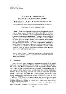
8th ASCE Specialty Conference on Probabilistic Mechanics and Structural Reliability
PMC2000-130
DIGITAL SIMULATION OF NON-GAUSSIAN STATIONARY PROCESSES USING KARHUNEN-LOEVE EXPANSION S.P. Huang, K.K. Phoon and S.T. Quek Department of Civil Engineering, National University of Singapore, Singapore 117576
[email protected],
[email protected] and
[email protected] Abstract A new simulation algorithm is developed for generating non-Gaussian processes with a specified marginal distribution function and covariance function.
It utilizes the Karhunen-Loeve (K-L) expansion for
simulation and an iterative mapping scheme to fit the target marginal distribution function. A stationary random process with Gamma marginal distribution is used to demonstrate the validity and convergence characteristics of the proposed algorithm.
Introduction Problems involving random processes are commonly encountered in various fields of engineering. Most random processes are assumed to be Gaussian both for simplicity and by virtue of the Central Limit Theorem. However, this simplification cannot be generalized to all situations. In some cases, the Gaussian assumption is not valid because observation data exhibit distinct non-Gaussian characteristics. Therefore, the simulation of non-Gaussian processes is of practical and theoretical importance. Simulation methods for Gaussian processes are quite well established. However, research on the simulation of non-Gaussian processes is comparatively limited. Yamazaki and Shinozuka (1988) proposed an iterative method for the generation of sample fields of a multi-dimensional non-Gaussian homogeneous stochastic field with a target power spectral density and marginal distribution function. Deodatis et al. (1998) extended the work done by Yamazaki and Shinozuka to the simulation of multi-variate, multidimensional non-Gaussian stochastic fields. Grigoriu (1998) also developed a simulation algorithm for generating non-Gaussian stationary translation processes with prescribed marginal distribution and covariance function. Karhunen-Loeve (K-L) expansion was previously used to represent Gaussian stationary or non-stationary processes (e.g., Huang et al., 1999). The present paper extends this representation to the case of non-Gaussian processes. A K-L representation-based simulation methodology will be proposed for generating both stationary and nonstationary non-Gaussian processes. It utilizes K-L expansion for the simulation of stochastic processes and an iterative mapping scheme to fit the non-Gaussian marginal distribution. The proposed method differs from other available techniques for generating non-Gaussian processes in four important aspects: (a) target covariance function is Huang, Phoon and Quek
1
maintained while the marginal distribution is updated iteratively, (b) processes with Gaussian-like marginal distribution can be generated almost directly without iteration, (c) distributions that deviate significantly from the Gaussian case can be handled efficiently, and (d) non-stationary non-Gaussian processes can be generated within the same unified framework. A stationary non-Gaussian process will be simulated to illustrate the algorithm and its performance. Karhunen-Loeve expansion Consider a random process ϖ ( x,θ ) defined on a probability space ( Ω , A, P) and indexed on a bounded domain D. Assume that the process has a mean ϖ (x) and a finite variance, E [ ϖ ( x ,θ ) − ϖ ( x )] 2 , that is bounded for all x ∈ D . The process can be expressed as ∞
ϖ ( x,θ ) = ϖ ( x) + ∑ λi ξ i (θ ) f i ( x)
(1)
i =1
in which λi and f i (x) are the eigenvalues and eigenfunctions of the covariance function C ( x1 , x2 ) . It has the following spectral decomposition ∞
C ( x1 , x2 ) = ∑ λi f i ( x1 ) f i ( x 2 )
(2)
i =1
and its eigenvalues and eigenfunctions are solutions of the homogenous Fredholm integral equation of the second kind given by
∫D C ( x1 , x2 ) f i ( x1 )dx1 = λi f i ( x2 )
(3)
Eq. (3) arises from the fact that the eigenfunctions form a complete orthogonal set satisfying the equation
∫D f i ( x) f j ( x)dx = δ ij
(4)
where δ ij is the Kronecker-delta function. The Fredholm integral equation can be solved analytically only under special circumstances. In most cases, numerical methods such as the Galerkin, collocation or Rayleigh-Ritz method are required (e.g., Huang et al., 1999). The parameter ξ i ( θ ) in Eq. (1) is a set of uncorrelated random variables which can be expressed as
ξ i (θ ) =
Huang, Phoon and Quek
1
λi
∫ [ϖ ( x,θ ) − ϖ ( x)] f i ( x)dx
(5)
D
2
with mean and covariance function given by E [ ξ i ( θ )] = 0
(6a)
E [ ξ i ( θ )ξ j ( θ )] = δ ij
(6b)
The series expansion in Eq. (1), referred to as the K-L expansion, provides a secondmoment characterization in terms of uncorrelated random variables and deterministic orthogonal functions. It is known to converge in the mean square sense for any distribution of ϖ ( x, θ ) (Van Trees, 1968). For practical implementation, the series is approximated by a finite number of terms, say M, giving M
ϖ M ( x,θ ) = ϖ ( x) + ∑ λi ξ i (θ ) f i ( x)
(7)
i =1
The corresponding covariance function is given by M
C M ( x1 , x 2 ) = ∑ λi f i ( x1 ) f i ( x 2 )
(8)
i =1
If ϖ ( x,θ ) is limited to a zero-mean Gaussian process, then an appropriate choice of { ξ i (θ ) } is a vector of zero-mean uncorrelated Gaussian random variables. For a random process ϖ ( x,θ ) with arbitrary distribution, the probability distribution of ξ i (θ ) may be estimated by integrating Eq. (5) numerically using any quadrature schemes. However, the integrand is obviously an unknown. Hence, an iterative procedure is required as discussed below. Simulation algorithm of non-Gaussian process The proposed algorithm to digitally generate sample functions of any non-Gaussian process is briefly described below. Full details are given elsewhere (Phoon et al., 2000). a. Select a target covariance function C ( x1 , x 2 ) and a marginal cumulative distribution function F. b. Set the random variables ξ i ( θ ) in the K-L expansion to satisfy Eq. (6) and to be identically F-distributed. c. Decompose the covariance function C ( x1 , x2 ) into its eigenvalues and eigenfunctions using Eq. (3). d. Generate N sample functions of the non-Gaussian process using the truncated K-L expansion as follows:
Huang, Phoon and Quek
3
(k ) ( x ,θ m ϖM
M
) = ϖ ( x ) + ∑ λi ξ i( k ) ( θ m ) f i ( x )
m = 1, 2, … N
(9)
i =1
where k = iteration number and m = sample number. e. Compute the simulated covariance and marginal cumulative distribution functions as shown below: ! (k ) 1 N (k ) (k ) CM ( x1 , x 2 ) = ∑ ϖ M ( x1 ,θ m ) − ϖ ( x1 ) ϖ M ( x 2 ,θ m ) − ϖ ( x 2 ) (10a) N m=1
[
][
! 1 FM( k ) ( y | x ) = N
]
∑ I (ϖ M( k ) ( x ,θ m ) ≤ y ) N
(10b)
m =1
where I ( event ) = indicator function = 1 if event is true and 0 otherwise. f. Transform each sample function so that the target marginal distribution is achieved:
[
]
! (k ) (k ) ( x ,θ m ) = F −1 FM( k ) ϖ M ( x ,θ m ) ζM
(11)
g. Compute the next generation of ξ i ( θ ) using Eq. (5) as follows:
ξ i( k +1 ) ( θ m ) =
1
λi
∫ [ζ M
(k )
]
(k ) ( x ,θ m ) − ζ M ( x ) f i ( x )dx
(12)
D
(k ) (k ) where ζ M = mean of ζ M ( x ,θ ) .
h. Standardize ξ i ( θ ) so that E [ ξ i2 ( θ )] = 1 . Note that E [ ξ i ( θ )] = 0 by virtue of Eq. (12). i. Apply the Latin Hypercube sampling technique (e.g., Florian, 1992) to reduce the correlation between ξ i ( θ ) . j. Repeat steps (d) through (i) until the sample functions achieved the target marginal distribution. Numerical example Numerical simulation of a non-Gaussian stationary stochastic process is performed to investigate the performance of the method. The following Gamma distribution with parameters p=4, q=0.5 is selected to illustrate the proposed simulation algorithm. The target covariance function is: C ( x1 , x 2 ) = e −|x1 − x2 |
2
Huang, Phoon and Quek
(13)
4
Figure 1a shows the target marginal distribution and the simulated distribution function of the non-Gaussian process at the first iteration. Because the assumed K-L random variables at the first generation are not correct, the simulated distribution function will not coincide with the target distribution function. During the iterative process, the random variables used to generate sample functions at the kth iteration are updated according to algorithm described above. Figure 1b compares the target marginal distribution function with the simulated distribution function computed from sample functions at the end of the iteration procedure (the second iteration). It can be seen that the two curves in Fig. 1b agree very well. Note that the proposed algorithm is very efficient for this example as the target distribution does not deviate significantly from the Gaussian case. In fact, iteration is not required to generate the above Gamma process if the error in the lower tail probability at the first iteration is considered to be acceptable. The target covariance function and the simulated covariance function computed from sample functions at the last iteration are compared in Fig. 2. The comparison is good as to be expected. In fact, the comparison will be good at any iteration by virtue of Eq. (8). The algorithm is also capable of generating a strongly nonGaussian process as illustrated elsewhere (Phoon et al., 2000). Conclusions A new simulation algorithm has been developed for generating stationary non-Gaussian processes with a specified marginal distribution and covariance function. It utilizes Karhunen-Loeve (K-L) expansion for simulation of stochastic processes and iterative mapping scheme to fit the marginal distribution. A stationary random process with Gamma marginal distribution was used to demonstrate the validity and performance of the proposed simulation algorithm. 1
1
0.9
0.9 target simulated
0.7
0.7
0.6
0.6
0.5 0.4
0.5 0.4
0.3
0.3
0.2
0.2
0.1
0.1
0 -4
-3
-2
-1
target simulated
0.8
probability (F)
probability (F)
0.8
0 1 values ( y)
2
3
4
0 -4
-3
-2
-1
0 1 values ( y)
2
3
4
Figure 1. Target and simulated distribution function in (a) the first and (b) the last (second) iteration.
Huang, Phoon and Quek
5
1 tar ge t s im u late d
0 .9
c o va r i a n c e
0 .8 0 .7 0 .6 0 .5 0 .4 0 .3
0
0 .1
0 .2
0 .3
0 .4
0 .5 lag
0 .6
0 .7
0 .8
0 .9
1
Figure 2. Target and simulated covariance function of Gamma process (last iteration).
References Deodatis G., Popescu R. & Prevost J.H. (1998), “Simulation of homogenous nonGaussian stochastic vector fields”, Probabilistic Engineering Mechanics, 13(1), 1-13. Florian, A. (1992), “An efficient sampling scheme: Updated Latin Hypercube Sampling”, Probabilistic Engineering Mechanics, 12(2), 123-130. Grigoriu, M. (1998), “Simulation of stationary non-gaussian translation processes”, Journal of Engineering Mechanics, ASCE, 124(2), 121-126. Huang S.P., Quek S.T. & Phoon, K.K. (1999). “Karhunen-Loeve Expansion for Representation and Simulation of Stationary and Non-stationary Gaussian Random Processes”, International Journal for Numerical Methods in Engineering (under review). Phoon, K.K., Huang S.P. & Quek S.T. (2000). “Simulation of Non-Gaussian Processes Using Karhunen-Loeve Expansion”, Journal of Engineering Mechanics, ASCE (under review). Yamazaki, F. & Shinozuka, M. (1988), “Digital generation of non-Gaussian stochastic fields”, Journal of Engineering Mechanics, ASCE, 114(7), 1183-1197. Van Trees, H.L. (1968), Detection, Estimation and Modulation Theory, Part 1, John Wiley & Sons, New York.
Huang, Phoon and Quek
6