Dimension Reduction and Variable Selection

2/13/2018

Leonardo Auslender –Ch. 1 Copyright 2004

Ch. 1.1-1

2/13/2018


Ch. 1.1-2

Positive Definite Matrix and definitions. Symmetric matrix with all positive eigenvalues. In the case of covariance and correlation matrices (that are symmetrical), all eigenvalues are real numbers. Correlation and covariance matrices must have positive eigenvalues, otherwise they are not of full rank  there are perfectly linear dependencies among the variables. For X data matrix of predictors, sample covariance = X’X = v. Generalized sample variance = det (v) (not much used). Since vars in X have different scales, could use instead correlation matrix, i.e., det (R).

2/13/2018


1.1-3

Principal Components Analysis (PCA) Technique for forming new variables from (typically) large ‘p’ data set, which are linear composites of the original. Variables.

Aim is to reduce dimension (‘p’) of the data set while minimizing the amount of information lost if we do not choose all the composites. Number of composites = number of original variables  problem of composite selection.

2/13/2018


Ch. 1.1-4

Web example: 12 observations.

2/13/2018


1.1-5

23.091 is variance of X1 ….

2/13/2018


1.1-6

Let’s create Xnew arbitrarily from x1 and x2.

2/13/2018


1.1-7

2/13/2018


1.1-8

Play with the angle to maximize the fitted variance.

2/13/2018


1.1-9

2/13/2018


1.1-10

2/13/2018


1.1-11

2/13/2018


1.1-12

Aim: find projections to summarize (mean centered) data. Approaches. 1) Find projections/vectors of maximum variance. 2) Find projections with smallest avg (mean-squared) distance between original and projections, which is equivalent to 1). Thus, maximize the variance by choosing ‘w’ (w is the vector of coeffs, x the original data matrix), where variance is given by:

2/13/2018


1.1-13

To maximize variance fitted by component w, requires w to be a unit vector, and thus w’w = 1 as constraint. Thus maximize with constraint, i.e., Lagrange multiplier method.

L( w,  )     ( w ' w  1) 2 w

L  w ' w 1  L  2vw  2 w w And setting them to 0, we obtain: 2/13/2018


1.1-14

w'w 1 vw   w  vw   w  0 Thus, ‘w’ is eigenvector of v & maximizing w is the one associated with largest eigenvalue. Since v (= x’x) is (p, p), there are at most p eigenvalues. Since v is covariance  it is symmetric  all eigenvectors orthogonal to each other. Since v positive matrix  all eigenvalues > 0.

2/13/2018


1.1-15

While these principal factors represent or replace one or more of the original variables, they are not just a one-to-one transformation,  inverse transformations are not possible.

NB: can obtain PCA without w’w = 1 constraint, but then standard PCA interpretation is not true.

2/13/2018


1.1-16

Detour on Eigenvalues, etc. Let A (n,n) , v (n, 1),  scalar. Note that A is not the typical rectangular data set but a square matrix, for instance, a covariance or correlation matrix. Problem: find  / A v =  v has nonzero solution. Note that A v is a vector, for instance, the estimated predictions of a linear regression. (For us, A is data, v is coefficients,  v linear transformation of coefficients).  called eigenvalue if nonzero vector v exists that satisfies equation.

Since v  0  |A -  I| = 0  equation of degree n in , determines values for  (notice that roots of equation could be complex). 2/13/2018


Ch. 1.1-17

Diagonalization. Matrix A diagonalizable  has n distinct eigenvalues. Then S (n,n) is diagonalizing matrix, with eigenvectors of A as elements, and D is diagonal matrix with eigenvalues of A as its elements. S–1AS = D  A = SDS–1, and A2 = (SDS–1) (SDS–1) = SD2S–1 Ak = (SDS–1) …. (SDS–1) = SDkS–1 Example: 30% of married women get divorced; 20% of single get married each year. 8000 M and 2000 S, and constant population. Find number of M and S in 5 years. v = (8000, 2000)’; A = {0.7 0.2 0.3 0.8} Eigenvalues = 1; .05. Eigenvectors: v1 = (2; 3)’ v2 = (1; -1)’ ,,,,,,,, A5 = SDS–1 = (4125, 5875)’ As k  , eigenvalues  (1; 0)  A   (4000; 6000)’

2/13/2018


Ch. 1.1-18

Detour on Eigenvalues, etc (cont. 2). Singular Value Decomposition (SVD) Notice that only square matrices can be diagonalized. Typical data sets, however, are rectangular. SVD provides necessary link.

A (m,n), m  n  A = UV’, U(m, m) orthogonal matrix (its columns are eigenvectors of AA’) (AA’ = U  V’V  U’ = U 2U’) V(n, n) orthogonal matrix (its columns are eigenvectors of A’A) (A’A= V  U’U  V’ = V 2V’)  (m,n) = diagonal ( 1, 0) , 1 = diag( 1  2 ….  n)  0.

’s called singular values of A.

2’s are eigenvalues of A’A.

U and V: left and right singular matrices (or matrices of singular vectors). 2/13/2018


Ch. 1.1-19

Principal Components Analysis (PCA): Dimension Reduction for interval-measure variables (for dummy variables, replace Pearson correlations by polychoric correlations that assume underlying latent variables. Continuous-dummy correlations are fine). PCA creates linear combinations of original set of variables which explain largest amount of variation.

First principal component explains largest amount of variation in original set; second one explains second largest amount of variation subject to being orthogonal to first one, etc.

PCi=V1i*X1+ V2i *X2+V3i*X3

X3

PC1

X2

PC3

PC2

X1 2/13/2018


Ch. 1.1-20

PC scores for each observation created by product of X and V, the set of eigenvectors.

Covariance/Correlation Matrix

XV =

 p   Vi1 X1i  i p1  V X i1 2 i  i 1   p  Vi1 X ni  i 1

p

V

i2

X 1i



V

i2

X 2i



i 1 p

i 1 p



V

i2

i 1

 X ni

 Vip X1i   i 1  p Vip X 2i    i 1    p Vip X ni    i 1 p



SVD of Covariance/Correlation Matrix = USVT

2/13/2018

Ch. 1.1-21 Leonardo Auslender –Ch. 1 Copyright 2004

PCA computed by performing SVD/Eigenvalue Decomp. on covariance or correlation matrix. Eigenvalues and associated eigenvectors extracted from covariance matrix ‘sequentially’. Each successive eigenvalue is smaller (in absolute value), and each associated eigenvector is orthogonal to previous one. Covariance/Correlation Matrix

X=

SVD of Covariance/Correlation Matrix = USVT

2/13/2018


Ch. 1.1-22

Amount of variation fitted by first k principal components can be computed in following way. i are eigenvalues of covariance/correlation matrix.  1 0    0    0

2 

0



0



2 

0











0

 k











0



0



0 0     0     p 

k

% Variation fitted =



i



j

i 1 p

 100%

j1

2/13/2018


Covariance or Correlation Matrix derivation? Overlooked point: results are different. Correlation matrix is the covariance matrix of the same data but in standardized form. Assume 3 variables x1 through x3. If Var(x1) = k (var (x2) + var(x3)) for large k, then x1 will dominate the first eigenvalue and the others would be negligible. Standardization implicit in correlation matrix treats all variables equally, because of unitary variance of each one. Recommendation: depends on focus of study, similar problem in clustering: outliers can badly affect standard deviation and mean estimations  standardized variables do not reflect behavior of original variable.

2/13/2018


Ch. 1.1-24

proc princomp data = fraud.fraud cov out = outp_princomp; var DOCTOR_VISITS FRAUD MEMBER_DURATION NO_CLAIMS OPTOM_PRESC TOTAL_SPEND ; run; proc corr data = outp_princomp; var prin1 prin2 prin3 DOCTOR_VISITS FRAUD MEMBER_DURATION NO_CLAIMS OPTOM_PRESC TOTAL_SPEND; run;

2/13/2018


Ch. 1.1-25

Eigenvalues

Eigenvalue

Difference

Proportion

Cumulative

125607670.56

125600984.82

1.00

1.00

6685.73

6635.81

0.00

1.00

49.93

47.23

0.00

1.00

2.70

1.53

0.00

1.00

1.17

1.04

0.00

1.00

0.00

1.00

1.00

6.00

Number 1 2 3 4 5 6

0.13

All

125614410.22

125607670.43

Variance Explained

1.3E8

1.0

1E8

0.8 Proportion

Eigenvalue

Scree Plot

7.5E7

5E7

0.6

0.4

2.5E7

0.2

0

0.0 1

2

3

4

5

Principal Com ponent

6

1

2

3

4

5

Principal Com ponent

Cumulative Proportion

Just one components fits all the variance. Leonardo Auslender –Ch. 1 Copyright 2004

6

Principal Comp # 1 vs # 2

Principal com p # 2

400

200

0

-200 -20000

0

20000

40000

60000

Principal com p # 1

2/13/2018


Ch. 1.1-27

Correlations Principal Components Variable DOCTOR_VISITS FRAUD MEMBER_DURATION NO_CLAIMS OPTOM_PRESC PRIN1 PRIN2 PRIN3 TOTAL_SPEND

Princ. Component # 1 Princ. Component # 2 Princ. Component # 3 0.10 -0.08 0.09 -0.03 0.05 1.00 0.00 0.00

1.00

0.19 -0.17

0.98

0.03

-0.02 -0.00 0.05

-0.11 0.00 1.00 0.00 -0.00

-0.05 0.00 0.00 1.00 -0.00

1.00

Three important dimensions: total spending, member Duration and doctor visits. Also note how principal components are uncorrelated Among themselves. Typically, interpretation not to ‘easy’, and number of PCs for later use has to be determined. Leonardo Auslender –Ch. 1 Copyright 2004

2/13/2018


Ch. 1.1-29

Data set used is Home Equity Loan. All continuous Variables (except for job, reason) are: BAD(binary target) -

Default or seriously delinquent

CLAGE -

Age of oldest trade line in months

CLNO -

Number of trade (credit) lines

DEBTINC -

Debt to income ratio

DELINQ -

Number of delinquent trade lines

DEROG -

Number of major derogatory reports

JOB -

Prof/exec, sales, manager, office, self, or other

LOAN -

Amount of current loan request

MORTDUE -

Amount due on existing mortgage

NINQ -

Number of recent credit inquiries

REASON -

Home improvement or debt consolidation

VALUE -

Value of current property

YOJ -

Years on current job.

2/13/2018


Ch. 1.1-30

Variables used in PCA are measured in interval scale. Variables are:

LOAN -

Amount of current loan request

MORTDUE -

Amount due on existing mortgage

VALUE -

Value of current property

YOJ -

Years on current job

CLAGE -

Age of oldest trade line in months

NINQ -

Number of recent credit inquiries

CLNO -

Number of trade (credit) lines

DEBTINC -

Debt to income ratio.

2/13/2018


Ch. 1.1-31

Eigenvalues report indicates that first four principal components fit %70.77 of variation of original variables.

2/13/2018


Ch. 1.1-32

Eigenvectors report contains V coefficients associated with each of original variables for first four principal components.

First principal component score for each observation is created by following linear combination. PC1=.3179*LOAN + .6005*MORTDUE +. 6054*VALUE + .0141*YOJ + .1827*CLAGE + .0606*NINQ + .3314*CLNO + .1574*DEBTINC

2/13/2018


Ch. 1.1-33

At this stage, it is customary to try to interpret the eigenvectors in terms of the original variables. The first vector had high relative loads in MORTDUE, VALUE and CLNO that indicates a dimension of financial stress (remember that there is no dependent variable, i.e., BADS does not play a role). Given “financial stress”, the second vector is a measure of “time effects” based on YOJ and CLAGE. And so on to the third and fourth vectors. Notice that the interpretation is based on the magnitude of the coefficients, without any guidelines as to what constitutes a high relative load. Therefore, with a large number of variables, interpretation is more difficult because the loads do not necessarily distinguish themselves as high or low. In next table, conditioning on value and mortdue, hardly afflects correlation between YOJ and CLAGE. Note that full analysis would require 2nd order partial correlations (not done here). 2/13/2018


1.1-34

1st component.

2/13/2018


1.1-35

Correlations

Corr Type Zero order, partial and semipartial Corrs Model Name

With Var

Variables

Cond. Var

M1

VALUE

YOJ

CLNO

YOJ

CLAGE

MORTDUE

PARTIAL SEMI_P Value Value

Value

-0.010 -0.010

0.138

0.138 0.202

CLNO

0.225

0.221

MORTDUE

0.236

0.231

VALUE

0.226

0.221

CLNO

0.025 MORTDUE

0.042

0.042

VALUE

0.013

0.013

MORTDUE

-0.088 CLNO

-0.095 -0.095

VALUE

-0.162 -0.162

VALUE

0.008 CLNO

-0.010 -0.010

MORTDUE

0.138

0.138

YOJ 2/13/2018

ZERO_O RDER


1.000 1.1-36

Interpretation: PCR1: high loadings for MORTDUE, VALUE and CLNO  financial aspect? PCR2: given PCR1, YOJ and CLAGE  time aspect?, etc. Note: nice to have inference on component loadings. When p large, very difficult. Also, when looking at PCR2 for interpretation, it is imperative to first remove the effects of the first component equation from all variables, before looking at correlations.

2/13/2018


1.1-37

PCA advantage; co-linearity is removed when regressing on principal components, which is called Principal Components Regression (PCR). Y

Y

X1

X2 2/13/2018

PC1

PC2 Leonardo Auslender –Ch. 1 Copyright 2004

Ch. 1.1-38

Principal Components Regression.

1)

Resulting model still contains all variables.

2) Similar to ridge regression , but with truncation (due to choice of vectors) instead of shrinkage of ridge. 3) “Look where there’s light” fallacy. We are not looking at original information.

2/13/2018


Ch. 1.1-39

2/13/2018


Ch. 1.1-40

Discussion on Principal components (PCs). •

Dependent variable is not used  No selection bias (i.e., dep var does not affect PCA, which is ‘good’.)

•

Very often PCs not interpretable in terms of original variables.

•

Dependent variable not necessarily highly correlated with vectors corresponding to largest eigenvalues (in var sel context, tendency to select top eigenvalues related eigenvectors is unwarranted).

•

Sometimes most highly correlated vector corresponds to smaller eigenvalue.

•

Common practice: choose eigenvectors corresponding to high eigenvalues  vector selection problem in addition to third point above (Ferre (1995) argues most methods fail. For newer version, see Guo et al, (2002), and Minka (2000) for Bayesian perspective). Foucart (2000) provides framework for “dropping” principal components in regression. For robust calculation, see Higuchi and Eguchi (2004). Li et al (2002) analyze L1 for Principal Components.

2/13/2018


Ch. 1.1-41

Discussion on Principal components (PCs) (cont. 1). •

Alternative to ‘ad-hoc’ PC selection, eigenvalues. See Johnstone (2001).

•

May be impossible to implement in present Tera-Giga-bases.

•

If error component components.

2/13/2018

in

data,

PC

inference

chooses


too

on

many

Ch. 1.1-42

INTERVIEW Question: Our data is mostly binaries. PCA? 2/13/2018


Ch. 1.1-43

2/13/2018


Ch. 1.1-44

Factor Analysis. Family of statistical techniques to reduce variables into small number of latent factors. Main assumption: existence of unobserved latent variables or factors among variables. If factors are partialled from observed vars, partial corrs among existent variables should be zero.

Each observed var can be expressed as weighted sum of latent components: y  a f  a f  ....  a f  e i

i1 1

i2 2

ik k

i

For instance, concept of frailty can be ascertained by testing strength, weight, speed, agility, balance, etc. Want to explain the component of frailty in terms of these measures. Very popular in social sciences, such as psychology, survey analysis, sociology, etc. Idea is that any correlation between pair of observed variables can be explained in terms of their relationship with latent variables.

FA as generic term includes PCA, but they have different assumptions.

2/13/2018


Ch. 1.1-45

Differences between FA and PCA. Difference in the definition of variance of the variable to be analyzed. Variance of variable can be decomposed into common variance, shared by other variables and thus caused by values of the latent constructs, and unique variance that include error component. Unique unrelated to any latent construct. “Common” Factor analysis (FA (CFA used for confirmatory later) or exploratory EFA) analyzes only common variance, PCA considers total variance without distinction of common and unique. In PCA, factors account for inter-correlations among variables, to identify latent dimensions. In PCA, we account for maximum portion of variation in original set of variables. FA uses notion of causality, PCA is free of that. PCA better when vars measured relatively error free (age, nationality, etc). If vars are only indicators of latent constructs (test score, response to attitude scale, or surveys of aptitudes)  CFA. PCs: composite variables computed from linear combinations of the measured variables. CFs: linear combinations of “common” parts of measured variables that capture underlying constructs. 2/13/2018


Ch. 1.1-46

EFA Rotations.

An infinite number of solutions is possible, which produce same correlation matrix, by rotating reference axes of the factor solution to simplify the factor structure and to achieve a more meaningful and interpretable solution. IDEA BEHIND: rotate factors simultaneously so as to have as many zero loadings on each factor as possible. Meaningful and interpretable demand analyst’s expertise. Orthogonal rotation: angle between reference axes of factors are maintained at 90 degrees; oblique no (when factors assumed to be correlated). In next slides, example with computer hardware sales data, comparing PCA with different FA alternatives. In FA case, negative eigenvalues  covariance matrix NOT positive definite  Cum fitted variation proportion > 1. Note PCA not affected.

2/13/2018


Ch. 1.1-47

EFA. PCA gives unique solution, FA different solutions depending on method & estimates of communality. While PCA analyzes Corr (cov) matrix, CFA replaces main diagonal corrs by prior communality estimates: estimate of proportion of variance of the variable that is both error-free and shared with other variables in matrix (there are many methods to find estimates). Determining optimal # factors: ultimately subjective. Some methods: Kaiser-Guttman rule, % variance, scree test, size of residuals, and interpretability. Kaiser-Guttman: eigenvalues >= 1. % variance of sum of communalities fitted by successive factors. Scree test: plots rate of decline of successive eigenvalues. Analysis of residuals: Predicted corr matrix similar to original corr. Possibly, huge graphical output. 2/13/2018


Ch. 1.1-48

Differences between FA and PCA, communalities. PCA analyzes original corr matrix with’1’ in main diagonal, i.e., total variance. FA analyzes communalities, given by common variance. Main diag of corr matrix is then replaced, with options

(SAS):

ASMC sets the prior communality estimates proportional to the squared multiple correlations but adjusted so that their sum is equal to that of the maximum absolute correlations (Cureton; 1968).

INPUT reads the prior communality estimates from the first observation with either _TYPE_=’PRIORS’ or_TYPE_=’COMMUNAL’ in the DATA = data set (which cannot be TYPE=DATA).

MAX sets the prior communality estimate for each variable to its maximum absolute correlation with any other variable.

ONE sets all prior communalities to 1.0. RANDOM sets the prior communality estimates to pseudo-random numbers uniformly distributed between 0 and 1.

SMC sets the prior communality estimate for each variable to its squared multiple correlation with all other variables. Final communalities: proportion of the variance in each of the original variables retained after extracting the factors. 2/13/2018


1.1-49

FA properties (SAS)

Estimation method: PRINCIPAL (yields principal components), MAXIMUM LIKELIHOOD MINEIGEN: Smallest eigenvalue for retaining a factor.

Nfactors: Maximum number of factors to retain. Scree: display scree plot.

Rotate

Priors.

2/13/2018


1.1-50

Additional Factor Methods and comparisons. EFA: explores possible underlying factor structure of set of observed variables without imposing preconceived structure on outcome. Aim: identify underlying factor structure.

Confirmatory factor analysis (CFA): statistical technique used to verify the factor structure of a set of observed variables. CFA allows to test hypothesis that relationship between observed variables and their underlying latent constructs exists. Researcher uses knowledge of theory, empirical research, or both, postulates relationship pattern a priori and then tests the hypothesis statistically.

Confirmatory factor models ( ≈ linear factor models) Item response models ( ≈ nonlinear factor models). 2/13/2018


1.1-51

2/13/2018


1.1-52

2/13/2018


1.1-53

EDA Cum fitted variation by Eigenvectors up to 50 Eigenvalues. Principal Components Analysis and/or Factor Analysis. M_ = M1_TRN_ASMC_NONE

M_ = M1_TRN_ASMC_VARIMAX

M_ = M1_TRN_MAX_NONE

M_ = M1_TRN_MAX_VARIMAX

M_ = M1_TRN_ONE_NONE

M_ = M1_TRN_ONE_VARIMAX

1.25 1.00 0.75

Cum proportion of fitted variation

0.50 0.25

1.25 1.00 0.75 0.50 0.25 M_ = M1_TRN_RANDOM_NONE M_ = M1_TRN_RANDOM_VARIM... 1.25 1.00 0.75 0.50 0.25 0

10

20

30

40

50 0

10

20

30

40

50 0

10

20

30

40

50

Eige nvalue #

2/13/2018

M1_TRN_ASMC_NONE M1_TRN_MAX_NONE M1_TRN_ONE_NONE Leonardo Auslender

–Ch. 1

M1_TRN_ASMC_VARIMAX M1_TRN_MAX_VARIMAX M1_TRN_ONE_VARIMAX Copyright 2004

1.1-54

EDA Scree Plot - Factor Analysis - Eigenvalues and Eigenv. differences. M_ = M1_TRN_ASMC_NONE

4 3 2 1 0

Eigenvalue

3 2 1 0

4.44

4.44

3.06 2.92 2.16 1.59 1.34 1.26 Diff. 0.85 0.69 0.58 0.56 0.52 0.50 0.42 0.35 0.28 0.25 0.19 0.16 0.14 0.12 0.11 0.04 0.02 0.01 0.00 0.00 0.00 0.00 0.00 0.00 0.00 0.00 0.00 0.00 0.00 0.00 0.00 0.00 0.00 0.00 0.00 0.00 0.00 0.00 0.00 0.00 0.00 0.00 0.00 0.00 0.00 0.00 0.00 0.00 0.00 0.00 0.00 0.00 0.00 0.00 0.00 0.00 0.00 0.00 0.00 0.00 -0.00 -0.01 -0.02 -0.05 -0.06 -0.06 -0.10 -0.15 -0.17 -0.20 -0.24 -0.34 Eigenv.

3.06 2.92 2.16 1.59 1.34 1.26 Diff. 0.85 0.69 0.58 0.56 0.52 0.50 0.42 0.35 0.28 0.25 0.19 0.16 0.14 0.12 0.11 0.04 0.02 0.01 0.00 0.00 0.00 0.00 0.00 0.00 0.00 0.00 0.00 0.00 0.00 0.00 0.00 0.00 0.00 0.00 0.00 0.00 0.00 0.00 0.00 0.00 0.00 0.00 0.00 0.00 0.00 0.00 0.00 0.00 0.00 0.00 0.00 0.00 0.00 0.00 0.00 0.00 0.00 0.00 0.00 0.00 -0.00 -0.01 -0.02 -0.05 -0.06 -0.06 -0.10 -0.15 -0.17 -0.20 -0.24 -0.34 Eigenv.

3.06 2.92 2.16 1.59 1.34 1.26 Diff. 0.85 0.69 0.58 0.56 0.52 0.50 0.42 0.35 0.28 0.25 0.19 0.16 0.14 0.12 0.11 0.04 0.02 0.01 0.00 0.00 0.00 0.00 0.00 0.00 0.00 0.00 0.00 0.00 0.00 0.00 0.00 0.00 0.00 0.00 0.00 0.00 0.00 0.00 0.00 0.00 0.00 0.00 0.00 0.00 0.00 0.00 0.00 0.00 0.00 0.00 0.00 0.00 0.00 0.00 0.00 0.00 0.00 0.00 0.00 0.00 -0.00 -0.01 -0.02 -0.05 -0.06 -0.06 -0.10 -0.15 -0.17 -0.20 -0.24 -0.34 Eigenv.

M_ = M1_TRN_MAX_VARIMAX

M_ = M1_TRN_ONE_NONE

M_ = M1_TRN_ONE_VARIMAX

3.06 2.92 2.16 1.59 1.34 1.26 Diff. 0.85 0.69 0.58 0.56 0.52 0.50 0.42 0.35 0.28 0.25 0.19 0.16 0.14 0.12 0.11 0.04 0.02 0.01 0.00 0.00 0.00 0.00 0.00 0.00 0.00 0.00 0.00 0.00 0.00 0.00 0.00 0.00 0.00 0.00 0.00 0.00 0.00 0.00 0.00 0.00 0.00 0.00 0.00 0.00 0.00 0.00 0.00 0.00 0.00 0.00 0.00 0.00 0.00 0.00 0.00 0.00 0.00 0.00 0.00 0.00 -0.00 -0.01 -0.02 -0.05 -0.06 -0.06 -0.10 -0.15 -0.17 -0.20 -0.24 -0.34 Eigenv. M_ = M1_TRN_RANDOM_NONE

4 3 2 1 0

4.58

4.58

3.40 3.23

3.40 3.23

2.33 2.03 1.83 1.65 1.47 1.26 1.19 1.11 1.05 1.04 0.99 Diff. 0.91 0.84 0.79 0.76 0.73 0.69 0.65 0.62 0.59 0.52 0.49 0.43 0.40 0.27 0.26 0.22 0.19 0.15 0.12 0.09 0.06 0.05 0.03 0.00 0.00 0.00 0.00 0.00 0.00 0.00 0.00 0.00 0.00 0.00 0.00 0.00 0.00 0.00 0.00 0.00 0.00 0.00 0.00 0.00 0.00 0.00 0.00 0.00 0.00 0.00 0.00 0.00 0.00 0.00 0.00 0.00 0.00 0.00 0.00 0.00 0.00 0.00 0.00 0.00 0.00 Eigenv.

2.33 2.03 1.83 1.65 1.47 1.26 1.19 1.11 1.05 1.04 0.99 Diff. 0.91 0.84 0.79 0.76 0.73 0.69 0.65 0.62 0.59 0.52 0.49 0.43 0.40 0.27 0.26 0.22 0.19 0.15 0.12 0.09 0.06 0.05 0.03 0.00 0.00 0.00 0.00 0.00 0.00 0.00 0.00 0.00 0.00 0.00 0.00 0.00 0.00 0.00 0.00 0.00 0.00 0.00 0.00 0.00 0.00 0.00 0.00 0.00 0.00 0.00 0.00 0.00 0.00 0.00 0.00 0.00 0.00 0.00 0.00 0.00 0.00 0.00 0.00 0.00 0.00 Eigenv.

M_ = M1_TRN_RANDOM_VARIMAX

4.13

4.19

3.06 2.79 2.13 1.91

2.99 2.90

1.24 1.14 1.00 0.95 0.90 Diff. 0.82 0.71 0.68 0.56 0.51 0.49 0.43 0.40 0.31 0.23 0.23 0.14 0.06 0.03 0.01 0.01 0.00 0.00 0.00 0.00 0.00 0.00 0.00 0.00 0.00 0.00 0.00 0.00 0.00 0.00 0.00 0.00 0.00 0.00 0.00 0.00 0.00 0.00 0.00 0.00 0.00 0.00 0.00 0.00 0.00 0.00 0.00 0.00 0.00 0.00 0.00 0.00 0.00 0.00 0.00 0.00 0.00 0.00 -0.07 -0.12 -0.13 -0.16 -0.23 -0.35 -0.39 -0.43 -0.48 -0.60 -0.61 Eigenv.

0

2/13/2018

M_ = M1_TRN_MAX_NONE

4.44

4.44 4

M_ = M1_TRN_ASMC_VARIMAX

20

40

60

80

1.85 1.62 1.52 1.13 1.07 1.00 Diff. 0.85 0.77 0.72 0.68 0.59 0.50 0.48 0.43 0.40 0.32 0.29 0.23 0.17 0.12 0.00 0.00 0.00 0.00 0.00 0.00 0.00 0.00 0.00 0.00 0.00 0.00 0.00 0.00 0.00 0.00 0.00 0.00 0.00 0.00 0.00 0.00 0.00 0.00 0.00 0.00 0.00 0.00 0.00 0.00 0.00 0.00 0.00 0.00 0.00 0.00 0.00 0.00 0.00 0.00 0.00 0.00 -0.01 -0.04 -0.09 -0.12 -0.17 -0.19 -0.24 -0.26 -0.27 -0.32 -0.40 -0.41 -0.59 -0.68 Eigenv.

0

20

40

60

80


0

20

40

60

80

1.1-55

7.5 # Factors selected

EDA

# of factors selected - Factor Analysis. 15.0

12.5

10.0

5.0

2.5

0.0

M N_ TR 1_

M N_ TR 1_

A _V AX

M RI

NE NO C_

VA C_

NE O _N AX

M

M

AX

IM AR _V M O ND RA N_ TR NE 1_ O M _N M O ND RA N_ TR AX 1_ M IM AR _V NE O N_ TR 1_ M NE O _N NE O N_ TR AX 1_ M RI M

M

M

AS N_ TR 1_

AS N_ TR 1_

AX

1.1-56 Leonardo Auslender –Ch. 1 Copyright 2004 2/13/2018

M

M

Model Name

2/13/2018


1.1-57

2/13/2018


1.1-58

Varimax Rotation. VARIMAX: orthogonal rotation that maximizes sum of variance of squared loadings (squared correlations between variables and factors). Orthogonality: Intuitively achieved if, (a) any given variable has a high loading on a single factor but near-zero loadings on the remaining factors and if (b) any given factor is constituted by only a few variables with very high loadings on this factor while remaining variables have near-zero loadings on this factor. a) and b)  factor loading matrix is said to have "simple structure," and varimax rotation brings the loading matrix closer to such simple structure (as much as the data allow). Each variable can be well described by a linear combination of only a few basis functions (Kaiser, 1958). In next slides, compare ORIGINAL with VARIMAX for different factors (F_).

2/13/2018


1.1-59

2/13/2018


1.1-60

2/13/2018


1.1-61

2/13/2018


1.1-62

2/13/2018


1.1-63

2/13/2018


1.1-64

All variables, And very messy.

2/13/2018


1.1-65

2/13/2018


1.1-66

2/13/2018


1.1-67

2/13/2018


1.1-68

From: https://www.linkedin.com/groups/4292855/4292855-6171016874768228353 Question about dimension reduction (factor analysis) for survey question set What would be the interpretation for a set of survey questions where rotation fails to converge in 25 iterations, and the non-rotated solution shows 2 clear factors with Eigenvalues above 2, but the scree plot levels out right at eigenvalue = 2 and the remaining (many) factors are quite close together?

Answers: 1. Well you first want to get the model to convergence. I usually increase the # of iterations to 500. 2. I would suggest its a one factor solution and the above 1 criteria is probably not appropriate. How many items/questions were there in your survey? Answer from poster: Thank you. I was able to do this with # iteration = 500. There are 14 factors with eigenvalues above 1, accounting for a total of 66.7% of the variance. I am still unsure what the interpretation would be - I've never had a dataset before that had so many factors. Too much noise? A lot of variability in survey response? 3. I think that "14 eigenvalues make just 2/3 of the variance" is a warning. It means to my experience that there are no large eigenvalues at all and that there are just "scree" eigenvalues. This can be an effect of having too many variables (= too high dimension). In this case an "automatic" dimensional reduction will necessarily fail and a visual dimensional reduction is due.

2/13/2018


1.1-69

It can also mean that the data cloud is more or less "spherical". This would mean that there are many columns (or rows) in the correlation matrix containing just values close to zero. One can easily "eliminate" such "circular" variables as follows a) copy the correlation matrix to an Excel sheet b) For each column calculate (sum of elements - 1) = rowsum c) sort the columns by descending rowsum d) take just the "top 20" or so variables with the largest rowsum e) do the analysis with the 20 variables and study the "scree plot"

Sorry, in step b) you should also calculate the maximal column element except the "1" on the diagonal. In step d) you should also add variables with a small rowsum but a relatively large maximal correlation. 4. I agree with stated above. Just FYI, use Bartlett sphericity test to formally check low correlation issue. Try also alternate the type of rotation. 5. Without knowing what you are measuring ... I can tell you about a similar situation I experienced ... it took a high number of iteration to converge, only one eigen value above 2, and a dozen or more above 1 that made no theoretical sense. I deleted all items with little response variability, and reran it ... and it came out more clearly as a homogeneous measure (1 factor). Once accepted that I was dealing with one factor, I was able to make some edits to the items, collected more data on the revised measure, and now have a fairly tight homogeneous measure.... where I really thought there would be 5 or so factors!

 MESSAGE: Extremely ad-hoc solutions are typical, not necessarily recommended  think before you rush in.. 2/13/2018


1.1-70

2/13/2018


Ch. 1.1-71

Basic Introduction Different approaches to clustering (there are other taxonomies) 1) disjoint (k-means); 2) non-disjoint hierarchical(agglomerative), 3) fuzzy, soft method or overlapping methods or model-based clustering (EM algorithm). Marketing prefers disjoint to separate customers completely (assuming independent observations). Archaeology prefers agglomerative because two nearby clusters might emerge from previous one in downward tree hierarchy (e.g., fossils in evolutionary science).

Agglomerative or hierarchical methods: typically bottom-up method. Start from individual observations and agglomerate upwards. Info on # of clusters not necessary, but impractical for large data sets. End result called dendogram, tree structure. Necessary to define distance, different distances  different methods.

Overlapping, fuzzy: methods that deal with data that cannot be completely separated or with probability statement attached to cluster membership. Won’t review top-down (divisive methods), overlapping or fuzzy methods. 2/13/2018


1.1-72

Why so many methods? If there are ‘n’ data points, and aim at clustering into ‘k’ clusters, there are kn / k! number of ways to do it,  brute force methods not adequate. For instance, k = 3, n = 100, the number of ways is 8.5896253455335 * 10 ** 46. For n = 1000, a computer cannot calculate it. And n = 1000, it is rather small data size at present. Heuristics used, such as k-means, especially.

Methods typically use Euclidean distance, but correlation distance is also possible.

2/13/2018


1.1-73

2/13/2018


1.1-74

Disjoint: K-means (McQueen, 1967) (most used clustering method in business) Key concept underlying cluster detection: similarity, homogeneity or closeness of OBSERVATIONS. Resulting implementation is based on similarity or dissimilarity of measures of distance. Methods typically greedy (one observation at time). Start with given number of requested clusters K, N data points and P variables. Continuous variables only. Algorithm determines K arbitrary seeds that become original location of clusters in P dimensions (there is variety of ways to change starting seeds). By using Euclidean distance function, allocate each observation to nearest cluster given by original seeds. Re-calculate centroid (cluster center of gravity). Re-allocate observations based on minimal distance to newer centroids and repeat until convergence given by maximum number of iterations, or until cluster boundaries remain unchanged. K-means typically converges quickly. 2/13/2018


Ch. 1.1-75

Outliers can have negative effects because calculated centroid would be affected. If outlier is itself chosen as initial seed, effect is paradoxical: analyst may realize that the relative scarcity of observations is an indication of an outlier. If outlier is not chosen initially, centroid is unavoidably affected. On the other hand, the distortion introduced may be such as to make such a conclusion difficult to reach. Further disadvantage: method depends heavily on initial choice of seeds  recommended that more than one run be performed but then difficult/impossible to combine results. In addition, # of desired clusters must be specified, which is in many situations the answer the analyst wants the algorithm to provide. # iterations must also be given.

More importantly, search for clusters is based on Euclidean distances that produce convex shapes. If ‘true’ cluster is not convex, K-means could not find that solution. 2/13/2018


Ch. 1.1-76

Number of Clusters, determination. Cubic clustering criterion (CCC) explained later with Ward method.

Elbow rule: for each ‘k’ clustering solution, find out % Between cluster variation over total variation at every K, and stop at point when increasing K does not decrease the ratio significantly (can also be used for WARD method later on).

Elbow point sometimes cannot be fully distinguished. WEB

2/13/2018


1.1-77

Alternatives:

K-medoids replaces mean by data points. In this sense, more robust to outliers but inefficient for large data sets (Rousseeuw and Kaufman, 1987). Resulting clusters are disjoint: merging two clusters does not lead to combined overall super-cluster. Since method is non-hierarchical, impossible to determine closeness among clusters.

In addition to closeness issue, it is possible that some observations may belong in more than one cluster and thus it would be important to report a measure of the probability belonging in a cluster. Originally created for continuous variables. Huang (1998) among others, extended algorithm to nominal variables. Next: Cluster graphs derived from canonical discriminant analysis. 2/13/2018


1.1-78

2/13/2018


1.1-79

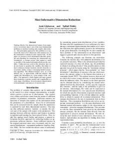
Fraud data set. Clusterin g solution Cluster 1 2 3 4 5 6 7

Total visits to a doctor # obs Mean 503 1452 203 165 491 150 662

1.81 -0.40 0.17 -0.01 -0.20 -0.18 -0.35

Fraudul No of ent Members claims Activity hip made yes/no duration recently

Number of opticals claimed

Total spent on opticals

Mean

Mean

Mean

Mean

Mean

-0.42 -0.50 -0.18 1.23 2.00 0.57 -0.49

0.48 -0.56 0.32 0.16 -0.43 -0.46 1.19

-0.18 -0.23 -0.21 3.77 0.01 -0.08 -0.25

-0.27 -0.12 -0.14 0.12 0.04 3.57 -0.27

-0.01 -0.18 2.79 -0.17 -0.41 0.45 -0.14

Is this great? NO, look at validation but Fraud difficult to work with. . Clusterin Fraudule No of Number g nt Member claims of Total solution ship made opticals spent on VALIDAT Total visits to a Activity doctor yes/no duration recently claimed opticals ION Cluster 1 2/13/2018

# obs 2334

Mean

Mean

Mean

Mean

Mean

Mean

-0.00

0.01

-0.01

0.00

-0.02

-0.02


Ch. 1.1-80

Hmeq K-means 3 clusters selected (ABC method,Aligned Box Criterion, SAS).

2/13/2018


1.1-81

Rescaled variable means by cluster (statistical inference, Parametric or otherwise, necessary to create profiles).

2/13/2018


1.1-82

2/13/2018


1.1-83

ods output ABCResults= abcoutput; proc hpclus data = training maxclusters = 8 maxiter = 100 seed = 54321 NOC = ABC (B= 1 minclusters = 3 align= PCA); input DOCTOR_VISITS /* FRAUD */ MEMBER_DURATION NO_CLAIMS OPTOM_PRESC TOTAL_SPEND; /* FRAUD OMITTED BEC. IT’S BINARY */ run;

proc sql noprint; select k into :abc_k from abcoutput; quit; proc fastclus data = training out = outdata maxiter = 100 converge = 0 replace = random radius = 10 maxclusters = 7 outseed = clusterseeds summary; var DOCTOR_VISITS /* FRAUD */ MEMBER_DURATION NO_CLAIMS OPTOM_PRESC total_spend; run; /* VALIDATION STEP, NOTICE validation AND clusterseeds. */ proc fastclus data = validation out = outdata_val maxiter = 100 seed = clusterseeds converge = 0 radius = 100 maxclusters = 7 outseed = outseed summary; var DOCTOR_VISITS /*FRAUD */ MEMBER_DURATION NO_CLAIMS OPTOM_PRESC TOTAL_SPEND; run; ; 2/13/2018


Ch. 1.1-84

2/13/2018


1.1-85

k-means assume: 1) the variance of the distribution of each attribute (variable) is spherical, i.e., E(x.x’) = σ2 IN. 2) all variables have the same variance; 3) the prior probability for all k clusters is the same, i.e. each cluster has roughly equal number of observations. Assumptions almost never verified, what happens when violated?

Plus, difficult if not impossible to ascertain best results. Examples in two dimensions, X and Y next. 2/13/2018


1.1-86

Non-spherical data.

2/13/2018


1.1-87

K-means solutions. X: centroids of found clusters.

2/13/2018


1.1-88

Instead, single linkage hierarchical clustering solution.

2/13/2018


1.1-89

Additional problems: Differently sized clusters. NO FREE LUNCH – NFL- (Wolpert, MacReady, 1997) “We have dubbed the associated results NFL theorems because they demonstrate that if an algorithm performs well on a certain class of problems then it necessarily pays for that with degraded performance on the set of all remaining problems”.

CANNOT USE SAME MOUSETRAP ALL THE TIME.  Hint: Verify assumptions, they ARE IMPORTANT. 2/13/2018


1.1-90

Interview Question: Aliens from far away prepare for invasion of Earth. Need to find whether intelligent creature live here and plan to launch 1000 probes for that purpose to random locations. Unknown to them, the oceans cover 71% of the Earth and the probe send back about the landing site and surroundings. Let us assume that just (some) humans are intelligent. The alien data scientist decides to use k-means on the data. Discuss how he/she would conclude whether there’s intelligent life on Earth (no sarcastic answers allowed)

2/13/2018


1.1-91

Agglomerative (hierarchical) clustering methods: Single linkage Centroid, Average Linkage and Ward.

2/13/2018


1.1-92

Agglomerative Clustering (standard in bio sciences). In single-linkage clustering (aka nearest neighbor or neighbor joining tree in genetics), distance between two clusters is determined by single element pair, namely those two elements (one in each cluster) that are closest to each other. And later compounds defined by min distance (see example below).

Shortest of these links that remains at any step causes fusion of two clusters whose elements are involved. Method is also known as nearest neighbor clustering: distance between two clusters is the shortest possible distance among members of clusters, or best of the friends. Result of clustering can be visualized as dendogram, which shows sequence of cluster fusion and distance at which each fusion took place. Distance or linkage factor given by

D( X ,Y )  min d ( x, y ) x X ,y Y

X and Y clusters, d is distance between 2/13/2018


1.1-93

In centroid method, (comonly used in biology) distance between clusters “l” and “r” is given by Euclidean distance between centroids. Centroid method is more robust than other linkage methods presented here, but has drawback of inversions (clusters do not become more dissimilar as we keep on linking up) .

In complete linkage (a.k.a. furthest neighbor) the distance between two clusters is longest possible distance between the groups, or the worst among the friends. In the case of average linkage method, the distance is the average distance between each pair of observations, one from each cluster. The method tends to join clusters with small variances. The Ward’s minimum variance method assumes that data set is derived from multivariate normal mixture, that clusters have equal covariance matrices and sampling probabilities. Tends to produce clusters with roughly same number of observations and based on the notion of information loss suffered when joining two clusters. Loss is quantified by Anova like Error Sums of Squares criterion. 2/13/2018


1.1-94

Example of complete linkage: Assume 5 observations with Euclidean distance as given by: 1 2 3 4 5

1 0 9 3 6 11

2

3

4

5

0 7 5 10

0 9 2

0 8

0

Let’s cluster closest observations, 3 and 5 (as 35), where distance between 1 and 35 is given by max distance (1 – 3, 1 – 5). After 6 steps, all observations are clustered. Dendograms (distance has height in Y axis) show agglomeration.

35 1 2 4 2/13/2018

35 0 11 10 9

1

2

4

0 9 6

0 5

0


1.1-95

Complete linkage

Single linkage

2/13/2018


1.1-96

How many clusters with agglomerative methods? Cut previous dendogram with horizontal line at specific point. No prevailing method, however. . E.g., 2 clusters.

Next: cluster solutions comparison (skipped bar charts of means of vars.) 2/13/2018


1.1-97

Cubic clustering criterion (Warren,1982). Assume 3 cluster solution left, and a reference distribution (right)

Reference distribution: hyper-cube of uniformly distributed random points aligned with principal components. Reference distribution typically be a hyper-cube. Heuristic formula to calculate error of distance based methods for k = 1 to k = top # clusters. CCC is difference error ( k = 1 ,,,,) to Top K – 1 to Error (top K). Largest CCC  desired k. Fails when variables are highly correlated. ABC method improves on CCC because it simulates multiple reference distribution, instead of just one heuristic as in CCC. 2/13/2018


1.1-98

Example, and Putting all Methods together.

2/13/2018


1.1-99

Hmeq methods comparison of canonical discr. Vectors.

2/13/2018


1.1-100

Notice missing ‘.’ cluster allocation. 2/13/2018


1.1-101

Previous slide: Hpclus (SAS proprietary cluster solution), Similar solutions between hpclus and k-means, very different from others. How to compare? Full disagreement. Since there is no initial cluster membership, no basis to obtain error rates.

There are many proposed measures, such as silhoutte coefficient, Adjusted Rand Index, etc. Final issues: Number of Clusters could be different across methods. Number of predictors, i.e., predictor selection, could be also different across methods. 2/13/2018


1.1-102

Methods for Number of Clusters determination. Ideal solution should minimize the “within cluster variation” (WCV) and maximize the between cluster variation (BCV). But WCV decreases and BCV increases with increasing number of clusters. WCV

K 1

Compromises: BCW n K CH index (Calinski et al, 1974): which is undefined for K = 1, i.e., no cluster case. GAP statistic (Tibshirani et al 2001): WCV ↓ as K ↑. Evaluate rate of decrease against uniformly distributed points. Milligan and Cooper (1985) compared many methods and up until 1985, CH was best. 2/13/2018


1.1-103

2/13/2018


1.1-104

Applications 1) Marketing Segmentation and customer profiling, even when supervised methods could be used.

2) Content based Recommender systems. E.g.: recommend based on movie categories preferred. E.g., cluster movie database and recommend within clusters. 3) Establish hierarchy or evolutionary path of fossils.

2/13/2018


1.1-105

Especially in marketing. 2/13/2018


1.1-106

Clustering and Segmentation in Marketing (easily Extrapolated to other applications). Definition: Segmentation: “viewing a heterogeneous market as a number of smaller homogeneous markets” (Wendell Smith, 1956). Bad practices. 1) Segmentation is descriptive, not predictive. However, business decisions made with eye to future (i.e., predictive). Business decisions based on segmentation are subjective and inappropriate for decision making, because segmentation only shows present strengths and weaknesses of brand (in marketing research), but doesn’t give and cannot give indications as to how to proceed. 2) CRM ISSUE: Segmentation assumes segment homogeneity, which contradicts basic CRM tenet of customer segments of 1. 2/13/2018


Clustering and Segmentation in Marketing 3) Competitors information and reactions are usually ignored at segment level. When Coca-Cola analyzed introduction of sweeter drink, only focused on Coca-Cola drinkers, forgetting customers’ perception of Coca Cola image. About AT&T, just look as to where AT&T is after 2000, after big mid-90 marketing failure based on segmentation, among other horrors.

4) Segmentation always excludes significant numbers of real prospects and conversely includes significant ones of nonprospects. In typical marketing situation, best and worst customers are easier to find, and the ones in between are non-easily classifiable. But segmentation imposes such a classification, and users do not remind themselves enough of the classification issues behind.

2/13/2018


Ch. 1.1-108

Clustering and Segmentation in Marketing Really unfortunate bad practices.

1) Humans categorize information to make it into comprehensible concepts. Thus, segments are typically labeled, and labels become “the” segments, regardless of segment accuracy, construction or stability of content, or changing market conditions. Worse yet, could well be that segments do not properly exist but that data derived clusters merely reflect normal variation (e.g., human evolution studies area of conflict in this). 2) Segments thus constructed cannot foretell changing market conditions, except once they have already taken place. Thus, you either gained, lost or kept customers. No amount of labeling, relabeling or label tweaking can be basis of successful operation in market place, since segments cannot predict behavior.

2/13/2018


Ch. 1.1-109

Clustering and Segmentation in Marketing. Really unfortunate bad practices. 3) Segments also derived from attitudinal data. Attitudes of customer base usually measured by way of survey opinions and/or focus groups. Derived information (psychographics) not easy to merge with created clusters from operational and demographic information.

4) Immediate temptation is to view whether segments derived from two very different sources have any affinity. This implies that it is necessary to ‘score’ customer base with psycho-graphically derived segments, in order to merge results. Accuracy of classification for this application has been traditionally very low. 5) Better practice: encourage usage of original clusters based on operational and demographic data as basis for obtaining psychographic information. 2/13/2018


Ch. 1.1-110

Clustering and Segmentation in Marketing 6) Finally, all models are based on available data. If aim is to segment entire US population, and one feature is NY Times readership (because that’s only subscription list available), useful mostly in NorthEast, but not so much in Kansas probably. In fact, it produces geographically based clustering, which may be undesirable or unrecognized effect.

Good practice. •

It can be systematic way to enhance marketing creativity, if possible.

Patting yourself in the back  2/13/2018


Ch. 1.1-111

Important note on how to work: Confirmatory Bias. Psychologists call ‘confirmatory bias’ the tendency to try to prove a new idea correct instead of searching to prove the new ideas wrong. This is a strong impediment to understanding randomness. Bacon (1620) wrote: “the human understanding, once it has adopted an opinion, collects any instances that confirm it, and though the contrary instances may be more numerous and more weighty, it either does not notice them or else rejects them, in order that this opinion will remain unshaken.” Thus, we confirm our stereotypes about minorities, for instance, by focusing on events that prove our prior beliefs and dismiss opposing ones. This is a serious contradiction to the ability of experts to judge in an unbiased fashion. Thus many times, we see what we want to see. Instead, per Doyle’s Sherlock Holmes: “One should always look for a possible alternative, and provide against it.” (to prove your point, The Adventure of Black Peter). 2/13/2018


Ch. 1.1-112

2/13/2018


1.1-113

1. Cluster Analysis using the Jaccard Matching Coefficient

2. Latent Class Analysis 3. CHAID analysis (class of tree methods, requires a target variable). 4. Mutual Information and/or Entropy. 5. Multiple Correspondence Analysis MCA.

Not reviewed in this class.

2/13/2018


1.1-114

Some Un-reviewed methods Mean shift clustering: non-parametric mode seeking algo. Density based spatial clustering of applications with noise (DBSCAN)

BIRCH: balanced iterative reducing and clustering using hierarchies. Gaussian Mixture Power iteration clustering (PIC) Latent Dirichlet allocation (LDA) Bisecting k-means

Streaming k-means …

2/13/2018


1.1-115

2/13/2018


1.1-116

Many analytical methods require the presence of complete observations, that is, if any feature/predictor/variable as a missing value, the entire observation is not used in the analysis. For instance, regression analysis requires complete observations. Failing to verify the completeness of a data set can lead to serious error, especially if we rely on UEDA notions of missingness.

For instance, the table below shows a simulation in which for a given set of number of variables ‘p’ (100, 350, 600, 850) and number of observations in the data set ‘n’ (1000, 1500, 2000), each variable has a probability of 0.01 and 0.11 of being missing. A priori these probabilities seem very low to cause much harm.

Table shows, however, that for modest ‘p’ = 100, resulting data sets have at least 60.93% missing values, and when ‘p’ reaches 350 almost all observations are missing. When univariate missingness is 11%, all observations are missing.

2/13/2018


1.1-117

Num Obs_in Database (n)

1000

Missing value analysis

Prob of missing value 0.01

0.11

2/13/2018

Num Vars_in Database (p) 100 350

# obs with_at least one missing value

1500 2000 # obs # obs % with_at % with_at missing least missing least obs_in one obs_in one databas missing databas missing e value e value

% missing obs_in database

619

61.90

914

60.93

1224

61.20

960

96.00

1449

96.60

1936

96.80

600

998

99.80

1496

99.73

1995

99.75

850

1000 1000

100.00 100.00

1500 1500

100.00 100.00

2000 2000

100.00 100.00

1000

100.00

1500

100.00

2000

100.00

600

1000

100.00

1500

100.00

2000

100.00

850

1000

100.00

1500

100.00

2000

100.00

100 350


1.1-118

A more subtle complication arises when missingness is not at random like in the table above. That is, assume that missingness in a variable of importance is related to its information itself, such as reported income is likely to be missing for high earners.

In this case, study of occupation by income, in which observations with missing values are skipped, would provide a very distorted picture. In other cases, data bases are created by merging different sources that were partially matched by some key indicator that could be unreliable (e.g., customer number)  data collection missingness).

2/13/2018


1.1-119

Missing values taxonomy (Little and Rubin, 2002)

We looked at the importance of treatment of missing values in a dataset. Now, let’s identify the reasons for occurrence of these missing values. They may occur at two stages: Data Extraction: It is possible that there are problems with extraction process. In such cases, we should double-check for correct data with data guardians. Some hashing procedures can also be used to make sure data extraction is correct. Errors at data extraction stage are typically easy to find and can be corrected easily as well.

Data collection: These errors occur at time of data collection and are harder to correct. They can be categorized in three types: Missing completely at random (MCAR): This is a case when the probability of missing variable is the same for all observations. For example: respondents of a data collection process decide that they will declare their earnings or weights after tossing a fair coin. In this case, each observation has an equal chance of containing a missing value. 2/13/2018


1.1-120

Missing at random (MAR): This is a case when a variable is missing at random regardless of the underlying value but probably induced by a conditioning variable. For example: age is typically missing in higher proportions for females than for males regardless of the underlying age of the individual. Thus, missingness is related only to the observed data.

Missing not at random (MNAR): the case of missing income above, that is, a variable is missing due to its underlying value. It also involves missingness that depends on unobserved predictors.

2/13/2018


1.1-121

Solving missingness in Data Bases. Case Deletion: It is of two types: List Wise Deletion and Pair Wise Deletion, used in the MCAR case, because otherwise a biased sample might occur. .

List-wise deletion removes all observations in which at least one missing value occurs. As we say above, the resulting sample size could be seriously diminished. Due to the disadvantage of list-deletion, pair wise deletion proceeds with analyzing all cases in which variables of interest are complete. Thus, if the interest centers on variables A and B to be correlated, analysis proceeds on those observations with non-missing values of variables A and B, regardless of missingness in other variables. If the study centers on different pairs of variables, then different sample sizes may result.

2/13/2018


1.1-122

Mean/ Mode/ Median Imputation: Imputation is a method to fill in the missing values with estimated ones. The objective is to employ known relationships that can be identified in the valid values of the data set to assist in estimating the missing values. Mean / Mode / Median imputation is one of the most frequently used methods. It consists of replacing the missing data for a given attribute by the mean, median (quantitative attribute) or mode (qualitative attribute) of all known values of that variable. It can be of two types: Generalized Imputation: In this case, we calculate the mean or median for all the complete values of that variable and then impute the missing values correspondingly. Conditional imputation: If missingness is known to differ by a third variable, obtain the mean/median/mode by the different values of the third variable and impute. Thus, in the case of missing age, obtain the statistics corresponding to males and females, and impute.

2/13/2018


1.1-123

Prediction Model:

Prediction model estimates values that will substitute missing data. In this case, divide our data set into two sets: One set with no missing values for the variable in question and another one with missing values. First data set become training data set of model while second data set with missing values is test data set and variable with missing values is treated as target variable. Next, create model to predict target variable based on other attributes of training data set and populate missing values of test data set. We can use regression, ANOVA, Logistic regression and various modeling technique to perform this. 2 drawbacks: 



2/13/2018

Model estimated values usually more well-behaved than true values, i.e., smaller variance. If there are no relationships with attributes in the data set and the attribute with missing values, then model will not be precise for estimating missing values. Leonardo Auslender –Ch. 1 Copyright 2004

1.1-124

KNN Imputation In this method of imputation, missing values of attribute are imputed using given number of attributes that are most similar to the attribute whose values are missing. Similarity of two attributes determined using distance function. It is also known to have certain advantage & disadvantages. Advantages: k-nearest neighbor can predict both qualitative & quantitative attributes Creation of predictive model for each attribute with missing data is not required Attributes with multiple missing values can be easily treated Correlation structure of data is taken into consideration Disadvantage: KNN algorithm very time-consuming in analyzing large database. It searches through all dataset looking for most similar instances. Choice of k-value is very critical. Higher value of k would include attributes which are significantly different from what we need whereas lower value of k implies missing out of significant attributes.

2/13/2018


1.1-125

Dummy coding. While not a solution, it recognizes the existence of the missing value. For each variable with a missing value anywhere in the data base, we create a dummy variable with value 0 when the corresponding value is not missing, and 1 when it is missing. The disadvantage is that the number of predictors can increase significantly. In some contexts, researchers drop the missing variables and work with the dummies instead. In most applied work, it is assumed that missingness is not of the MNAR type. In all cases of imputation, we should note that the imputed values may shrink the variance of the individual variables. Thus, it is appropriate to ‘contaminate’ these estimates with a random component, for instance, a normally distributed random error for a continuous variable. ISSUE

If also want to transform data, decide whether to transform and then impute, or instead to impute raw data and then work with transformations.

2/13/2018


1.1-126

2/13/2018


1.1-127

Dataset 'bbny' with 8166 Obs Var_1

Variable

Model Name M1_INTERVAL_VARS

Var_2

M1_INTERVAL_VARS

Var_3

M1_INTERVAL_VARS M1_IMPUTED_INTERV AL_VARS

Var_4


Var_5


Var_6


Var_7


# Nonmis s Obs % Missing

Mean

Std of Mean

Mode

1,430

82.49

64.681

3.545

3.990

8,166

0.00

136.898

2.329

49.990

5,014

38.60

520.282

9.850

49.990

8,166

0.00

447.642

6.156

273.053

3,741

54.19

0.261

0.029

0.000

8,166

0.00

0.135

0.014

0.000

4,358

46.63

0.207

0.022

0.000

8,166

0.00

0.122

0.012

0.000

7,344

10.07

11.770

0.849

0.000

8,166

0.00

10.823

0.765

0.000

8,164

0.02

12.207

0.246

5.000

8,166

0.00

12.207

0.246

5.000


Distr of imputed Variables same as that of original variables. 2/13/2018


1.1-129

2/13/2018


1.1-130

Outliers and Variables Transformations. Outlier and variable transformation analysis are sometimes included as part of EDA. Since both topics must be understood in context of modeling of dependent or target variable, we will state some general issues. Wrongly asserted that analyst should verify existence of outliers and then blindly remove or impute them to more ‘accomodating’ values without reference to problem at hand. E.g., sometimes argued that registered data point for man’s height of 8 feet must be wrong or outlier, except that in antiquity there is historical evidence for that occurrence. In present times, tendency to disregard income levels above say, $50 million, when mean value in sample is probably $50,000. However, extreme values are real, and probably most interesting. On the other hand, age of 300 years or more is quite suspicious, unless we are referring to a mummy. In cases when data points in reference to the model at hand can and should be disputed, outliers can then be treated as if they were missing values, and most likely of the MNAR kind. Thus, mean, median or mode imputation should not be considered as the immediate solution. 2/13/2018


1.1-131

If we view the data bi-variately, data points that otherwise would not be considered to be outliers, could be bi-variate outliers. For instance, weight of 400 pounds and 3 years of age are possible when considered univariately, but highly suspicious in one individual.

In the area of variable transformations, we already saw the convenience of standardizing all variables in the case of principal components and/or clustering. There are other cases when the analyst implements single variable transformations, such as taking the log, which lowers the variance of the variable in question.

Again, it is important to reiterate that most information is not of univariate but of multi-variate importance. Further, there is no magic in trying to obtain univariate or multi-variate normality, as it may be thought for the case of inference, since inference does not require that variable information be normally distributed. 2/13/2018


1.1-132

Sources of outlierness: 

Data Entry or data processing Errors, such as errors in programming when merging data from many different sources.



Measurement Error due to faulty measuring device, for instance.



Experimental Error: Another cause of outliers is experimental error. For example: In a 100m sprint of 7 runners, one runner missed out on concentrating on the ‘Go’ call which caused him to start late. Hence, this caused the runner’s run time to be more than other runners. His total run time can be an outlier.



Intentional misreporting: Adverse effects of pharmaceuticals are well known to be under-reported.



Sampling error, when information unrelated to the study at hand is included. For instance, male individuals included in a study on pregnancy.

2/13/2018


1.1-133

Effects of Outliers.

Outliers may distort analysis as is well known in the case of linear and logistic regressions. They also distort inference since by their very nature, they affect mean calculations, which are the focus of inference in many instances. We will review outlier detection while reviewing modeling methods. There are “robust’ modeling methods that are (more) impervious to outliers, such as robust regression. Tree modeling methods and their derivatives are also impervious to outliers.

2/13/2018


1.1-134

Variables transformations and MEDA. Raw data sets can have variables or features that are not directly useful for analysis. For instance, age coded in terms of “infant”, “teen’, etc. do not connote the underlying ordering, and can be more easily denoted in terms of an ordered sequence of numbers. In a different example, if we are studying volumes, variables that may affect them might require to be raised to the third power to correspond to the cubic nature of volumes. In short, variable transformation belongs in the MEDA realm because we are interested in how the transformed variable relates to others.

The topic of variable transformations is also called variable engineering because different disciplines add more jargon to each other. 2/13/2018


1.1-135

Some prevailing practices in variable transformation (see previous sections for more detail). 1) Standardization (as we saw in clustering and also principal components): it does not alter the variable distribution but rescales and standardizes to a common variance of 1. 2) Linearization, via logs: If the underlying model is deemed to be multiplicative, log transformation turns it into an additive model. Likewise for skewed distributions, as in the case of count variables. And obviously, sometimes the required transformation is the square, cubic or square root of the original variable. 3) Binning: usually done by cutting the range of a continuous variable into sub-ranges that are deemed to be uniform or more representative, for instance, in the case of age mentioned previously. 4) Dummying: Used typically with a categorical variable, such as one denoting color. Some modeling methods, such as regression based methods, require that if there are k classes of a categorical variable, (k-1) dummy variables (0/1) variables be derived. Tree methods do not require this construction.

2/13/2018


1.1-136

2/13/2018


1.1-137

1. A baseball bat and a ball cost $1.10 together, and the bat costs $1 more than the ball. What’s the cost of the ball? 2. In a 2007 blog, David Munger (as stated by Adrian Paenza of Pagina 12, 2012/12/21), proposes the following question: without thinking more than a second, choose a number between 1 and 20 and ask friends to do the same and tally all the answers. What is the distribution. 3. Three friends go out to dinner and the bill is $30. They each contribute $10 but the waiter brings back $5 in $1 dollar bills because there was an error and the tab was just $25. They each take $1 and give $2 to the waiter. But then, one of them says that they each paid $9 for a total of $27, plus the $2 tip to the waiter, which all adds up to $29 and not to the $30 that they originally paid. Where is the missing dollar? 4. Explain the relevance of the central limit theorem to a class of freshmen in the social sciences who barely have knowledge about statistics.

5. What can you say about statistical inference when sample is whole population? 6. What is the number of barber shops in NYC? (coined by Roberto Lopez of Bed, Bath & Beyond, 2017). 2/13/2018


1.1-138

In a very tiny city there are two cab companies, the Yellows (with 15 cars) and the Blacks (with 75 cars). The core of the problem is that there was an accident during a drizzly night and that all cabs were on the streets. 7)

A witness testifies that a yellow cab was guilty of the accident. The police check his eyesight by showing him yellow and black cab pictures and he identified them correctly 80% of the time. That is, in one case out of five he confused a yellow cab for a black cab or vice-versa. Knowing what we know so far, is it more likely that the cab involved in the accident was yellow or black? The immediate unconditional answer (i.e., based on the direct evidence shown) is that there is 80% probability that the cab was yellow. State your reasoning, if any.

8) Can a random variable have infinite mean and/or variance? 9) State succintly differences between PCA, FA and clustering. 2/13/2018


1.1-139

References Bacon F. (1620): Novum Organon, XLVI. Calinski T., Harabasz J. (1974): A dendrite method for cluster analysis, Communications in Statistics Huang Z. (1998): Extensions to the k-Means Algorithm for Clustering Large Data Sets with Categorical Values, Data Mining and Knowledge Discovery 2. Johnstone I. (2001): On the Distribution of the largest eigenvalue in Principal Components Analysis, The Annals of Statistics, vol. 29, # 2.

MacQueen J. (1967): “Some Methods for Classification and Analysis of Multivariate Observations.” In Proceedings of the Fifth Berkeley Symposium on Mathematical Statistics and Probability, Volume 1: Statistics, 281–97. Berkeley, Calif.: University of California Press. Milligan G., Cooper M. (1985): An examination of procedures for determining the number of clusters in a data set, Psychometrika, 159-179. Tibshirani R. et al (2001): Estimating the number of clusters in a data set via the gap statistic., J. R. Statis. Soc. B, pp. 411-423

2/13/2018


1.1-140

2/13/2018


Ch. 1.1-141