sufficient dimension reduction based on normal and

SUFFICIENT DIMENSION REDUCTION BASED ON NORMAL AND WISHART INVERSE MODELS

A THESIS SUBMITTED TO THE FACULTY OF THE GRADUATE SCHOOL OF THE UNIVERSITY OF MINNESOTA BY

LILIANA FORZANI

IN PARTIAL FULFILLMENT OF THE REQUIREMENTS FOR THE DEGREE OF DOCTOR OF PHILOSOPHY

R. DENNIS COOK, Advisor

December, 2007

c °Liliana Forzani 2007

UNIVERSITY OF MINNESOTA

This is to certify that I have examined this copy of a doctoral thesis by

Liliana Forzani

and have found that it is complete and satisfactory in all respects, and that any and all revisions required by the final examining committee have been made.

R. Dennis Cook Name of Faculty Adviser

Signature of Faculty Adviser

Date

GRADUATE SCHOOL

0.1

Acknowledgments

I would like to thanks my thesis advisor, Dennis Cook. He always welcomed my questions and doubts (and they were not so few). His insights, contagious enthusiasm and intensity were a big part of what made possible for me to complete this work. I hope to carry some of these attributes with me in my professional life, as I know I will carry all the knowledge he taught me. ¡ Gracias ! Thanks (orderless) to Carlos, who introduced me to the data world and shared with me so many principal component analysis conversations... to Professor Eaton for teaching me, among other things, to resist the temptation to take the derivative every time there is a function to maximize... to John, Pedro, Roberto and Yongwu, who were always willing to have discussions (even about statistics)... to Marcela who generously gave me the bird-plane-car data... to Li Bing for giving me the code for directional reduction to Aaron, who was always there for a graphical, LATEX or statistics question... to Marco who in order to share the joy I was having doing this thesis made the beautiful mathematical drawing that is in this thesis... to Davide, for the coffee, the food and being the alma of the fourth floor... to my dear friends from IMAL (Instituto de Matem´atica Aplicada ”Litoral”), who are still waiting for me... to my little friends, Bruno, Gaby, Leo, Manon, Palito, who together with Marco are the smiles of my life outside the academics...(and their parents too) to Edu, for making this journey with me... to Nancy, she knows why...

i

To Bera, Edu, Javier and Marco ....

ii

Contents 0.1

Acknowledgments . . . . . . . . . . . . . . . . . . . . . . . . . . . . .

i

Dedication

ii

1 Introduction

1

2 Models and their attached reductions

5

2.1

Normal reductive models with constant variance . . . . . . . . . . .

5

2.2

Normal reductive models with non-constant variance . . . . . . . . .

11

2.3

Wishart reductive models . . . . . . . . . . . . . . . . . . . . . . . .

14

2.4

A look of functional data analysis and dimension reduction . . . . .

18

3 Normal inverse models with constant variance: the general case

30

3.1

Estimation under model PFC∆

. . . . . . . . . . . . . . . . . . . .

31

3.2

Relationships with other methods . . . . . . . . . . . . . . . . . . . .

33

3.3

Structured ∆ . . . . . . . . . . . . . . . . . . . . . . . . . . . . . . .

37

3.4

Inference about d . . . . . . . . . . . . . . . . . . . . . . . . . . . . .

38

3.5

Testing predictors

. . . . . . . . . . . . . . . . . . . . . . . . . . . .

39

3.6

Robustness . . . . . . . . . . . . . . . . . . . . . . . . . . . . . . . .

40

3.7

Simulation results

. . . . . . . . . . . . . . . . . . . . . . . . . . . .

41

3.8

Conclusions . . . . . . . . . . . . . . . . . . . . . . . . . . . . . . . .

46

iii

4 Normal inverse models with constant variance: mean and variance connection

62

4.1

Variations within model (2.4) . . . . . . . . . . . . . . . . . . . . . .

63

4.2

Relationships with other methods . . . . . . . . . . . . . . . . . . . .

64

4.3

Estimation . . . . . . . . . . . . . . . . . . . . . . . . . . . . . . . .

68

4.4

Simulations and data analysis illustrations . . . . . . . . . . . . . . .

74

4.5

Discussion . . . . . . . . . . . . . . . . . . . . . . . . . . . . . . . . .

78

5 Normal inverse models with non-constant variance

84

5.1

Estimation of Sα when d is known . . . . . . . . . . . . . . . . . . .

85

5.2

Choice of d . . . . . . . . . . . . . . . . . . . . . . . . . . . . . . . .

88

5.3

Testing Variates

. . . . . . . . . . . . . . . . . . . . . . . . . . . . .

89

5.4

Comparing with SIR and SAVE . . . . . . . . . . . . . . . . . . . . .

91

5.5

Is it a bird, a plane or a car? . . . . . . . . . . . . . . . . . . . . . .

94

5.6

Discussion . . . . . . . . . . . . . . . . . . . . . . . . . . . . . . . . .

98

6 Wishart inverse models

110

6.1

Relationship with principal components . . . . . . . . . . . . . . . . 111

6.2

Estimation of C with d Specified . . . . . . . . . . . . . . . . . . . . 113

6.3

Choice of d . . . . . . . . . . . . . . . . . . . . . . . . . . . . . . . . 115

6.4

Testing Variates

6.5

Garter Snakes . . . . . . . . . . . . . . . . . . . . . . . . . . . . . . . 119

6.6

Discussion . . . . . . . . . . . . . . . . . . . . . . . . . . . . . . . . . 121

. . . . . . . . . . . . . . . . . . . . . . . . . . . . . 117

7 Functional Data Analysis and Dimension Reduction

127

7.1

Introduction . . . . . . . . . . . . . . . . . . . . . . . . . . . . . . . . 127

7.2

The setting in Ferr´e and Yao (2005) . . . . . . . . . . . . . . . . . . 128

7.3

The results . . . . . . . . . . . . . . . . . . . . . . . . . . . . . . . . 130

7.4

Conclusions . . . . . . . . . . . . . . . . . . . . . . . . . . . . . . . . 132

iv

8 Further work and work in progress

134

8.1

Improving the mean-variance model for non-constant variance . . . . 134

8.2

Other models reducing the variance . . . . . . . . . . . . . . . . . . . 135

8.3

Several response variables . . . . . . . . . . . . . . . . . . . . . . . . 139

8.4

Minimal sufficiency for non-constant variance . . . . . . . . . . . . . 140

8.5

Functional data analysis . . . . . . . . . . . . . . . . . . . . . . . . . 142

Bibliography

158

v

List of Tables 4.1

Simulation results with alternative error distributions . . . . . . . .

6.1

Empirical distribution of db in percent. . . . . . . . . . . . . . . . . . 117

6.2

Simulation results on the level of the variate test using the likelihood ratio statistic Λd (H0 )

76

. . . . . . . . . . . . . . . . . . . . . . . . . . 118

vi

List of Figures 3.1

Tests of a diagonal ∆: The x-axis represents sample size and the y-axis the fraction F of time the null hypothesis is not rejected . . .

3.2

Inference about d, for d = 2 vs n: The x-axis is the sample size n. The y-axis is the fraction F (2) of runs in which d = 2 was chosen . .

3.3

42

43

Inference about d: The x-axis is the number of predictors p. The y-axis for Figures a and b is the fraction F (2) of runs in which d = 2 was chosen; for Figure c it is the fraction F (2, 3) of runs where d = 2 or 3 was chosen; for Figure d it is the fraction F (2, 3, 4) of runs where d = 2, 3 or 4 was chosen. . . . . . . . . . . . . . . . . . . . . . . . . .

3.4

44

Testing Y independent of X2 given X1 : The x-axis is the sample size and the y-axis is the fraction of runs in which the null hypothesis is not rejected. . . . . . . . . . . . . . . . . . . . . . . . . . . . . . . . .

45

4.1

Percentage of correct classifications versus the indicated variable. . .

75

4.2

b 1 and R b1 with separate Pea Crab data: Plots of the first LDA variate L density estimates for mussels with a Pea Crab (right density) and for mussels without a Pea Crab (left density). . . . . . . . . . . . . . . .

4.3

77

b1 and R b2 for the data Plots of the first two estimated reductions R from the Australian Institute of Sport. The curves are lowess smooths with tuning parameter 0.6.

. . . . . . . . . . . . . . . . . . . . . . .

vii

78

5.1

b Quartiles (a) and median (b) of the cosine of the angle between α and α versus sample size . . . . . . . . . . . . . . . . . . . . . . . . .

5.2

87

Inference about d: The x-axis is the sample size for each population. Figures a and b are for Case (i) where d = 1 and Figures c and d are for Case (ii) where d = 2. The y-axis for Figures a is the fraction F (1) of runs in which d = 1 was chosen; for Figure b is the fraction F (1, 2) of runs where d = 1 or 2 was chosen. For Figure c the y-axis is the fraction F (2) of runs where d = 2 was chosen and Figure d it is the fraction F (2, 3) of runs where d = 2, 3 was chosen. . . . . . . .

5.3

90

Comparing NEW method with SIR and SAVE: X ∼ N (0, Ip ) with p = 8. The x-axis is a from 1 to 10. For Figures a, b and c the sufficient reduction is α = (1, 0, 0, 0, 0, 0, 0, 0) and the y-axis represent the first coordinate of the estimation for the sufficient reduction. For Figure d the y-axis represent the maximum angle between the true subspace and the estimate one. . . . . . . . . . . . . . . . . . . . . .

93

5.4

Directions for BIRDS-PLANES using SIR, SAVE and DR . . . . . .

95

5.5

Two first NEW directions for BIRDS-PLANES . . . . . . . . . . . .

96

5.6

Directions for BIRDS-PLANES-CARS . . . . . . . . . . . . . . . . .

99

5.7

A 2-D projection of the 3-D plot when we consider three directions in DR for BIRDS-PLANES-CARS . . . . . . . . . . . . . . . . . . . 100

5.8

First two directions of NEW for BIRDS-PLANES-CARS . . . . . . . 101

5.9

Directions for BIRDS-PLANES-CARS without outliers . . . . . . . . 101

5.10 First two directions of NEW for BIRDS-PLANES-CARS without outliers . . . . . . . . . . . . . . . . . . . . . . . . . . . . . . . . . . . . 102 6.1

b Quartiles (a) and median (b) of the cosine of the angle between α and C versus sample size. . . . . . . . . . . . . . . . . . . . . . . . . 114

viii

Chapter 1

Introduction Many statistical problems deal with the study of the conditional distribution of a response Y given a predictor of vectors X ∈ Rp or with the relationship of a set of predictors X in different populations Y = 1, . . . , h. When the number of predictors is large, almost all of the methods used to study these relationships include some type of dimension reduction for X. Principal components is the dominant method of dimension reduction across the applied sciences, although there are other established and recent statistical methods that can be used in these regression settings, as for example, partial least squares (Wold, 1975; Helland, 1990), projection pursuit (Huber, 1985), and sparse methods based on the lasso (Tibshirani, 1996). Among the methods under the paradigm of sufficient dimension reduction for studying intrinsically low-dimensional regressions without requiring a pre-specified model, we can include sliced inverse regression (SIR; Li, 1991), sliced average variance estimation (SAVE; Cook and Weisberg, 1991), minimum average variance estimation (MAVE; Xia, et al. 2002), contour regression (Li, Zha and Chiaromonte, 2005), inverse regression estimation (Cook and Ni, 2005), Fourier methods (Zhu and Zeng, 2006), and a variety of methods based on marginal moments like principal Hessian directions (Li, 1992), iterative Hessian transformations (Cook and Li, 2002, 2004), and Directional Regression (DR; Li and Wang, 2007). These methods are semi-parametric or 1

non-parametric estimation techniques with limited inference capabilities relative to those typically associated with parametric modeling and many of them are designed to either focus or broaden the estimative target of other methods. In this thesis we work under the umbrella of the sufficient dimension reduction paradigm. Continuing a line of reasoning initiated by Cook (2007a), who derived principal components regression from the likelihood when X|Y follows a normal distribution, we develop a model-based approach to dimension reduction. In contrast to past studies, which focused on developing methodology with few assumptions, our goal is to discover structures in the data that allow increased efficiency. The following definition provides a conceptual foundation for sufficient dimension reduction and for the models we develop. Definition 1.0.1 (Cook, 2007a) A reduction R : Rp → Rq , q ≤ p, is sufficient for Y |X if it satisfies one of the following three statements: (i) inverse reduction, X|(Y, R(X)) ∼ X|R(X) (ii) forward reduction, Y |X ∼ Y |R(X) (iii) joint reduction, X where

Y |R(X)

indicates independence and ∼ means identically distributed.

The choice of a reductive paradigm depends on the stochastic nature of X and Y . If the values of X are fixed by design, then forward regression (ii) seems the natural choice. In discriminant analysis X|Y is a random vector of features observed in one of a number of populations indexed by Y . In this case the inverse regression (i) is perhaps the only reasonable reductive route. For the case of (Y, X) having a joint distribution the three statements in Definition 1.0.1 are equivalent. In this last case we are free to estimate a reduction inversely or jointly and then pass the estimated reduction to the forward regression without additional structure.

2

Part of this thesis is based on models for the inverse regression X|Y , where X is a vector of predictors. When (X, Y ) has a joint distribution, we use them to study the sufficient reduction for the regression of Y |X. When Y is fixed indicating different populations, we use them to study the behavior of the predictors X in each of those populations. Using as a starting point the hypothesis of normality of X|(Y = y), we developed a methodology for the forward regression of Y |X in the first case, and for discrimination in the second one. This methodology includes finding the dimension of the central subspace, maximum likelihood estimation for a basis of the central subspace, testing for predictors and prediction, among others. Chapters 3, 4 are dedicated to the case when Var(X|Y ) is constant. In Chapter 5 we consider the case of non-constant variance. For each of these models, we study estimation, inference procedures and connections and relations with other models. Although we adopt a model-based approach, these models seems to be robust to a range of variations in the error distribution. Later, in Chapter 6, we concentrate in sufficient reductions for covariance matrices. In that context we study covariance matrices for different values of Y and how to define and estimate a sufficient reduction. Having done that, we concentrate on estimation of the dimension of the central subspace. We also study maximum likelihood estimators for a basis of the central subspace, as well as the associated methodology. In Chapter 7 we move away from finite dimension and we give some basic results that will allow us to extend the results of this thesis to the context of Functional Data Analysis. Finally, Chapter 8 is about work in progress and further work for the finite and infinite dimensional cases. The following notation will be used repeatedly in our exposition. For positive integers r and p, Rr×p stands for the class of all matrices of dimension r × p, Sr×r denotes the class of all symmetric r × r matrices and S+ r the subclass of positive definite matrices of dimension r. For α ∈ Rp×d , d ≤ p with orthogonal columns,

3

α0 ∈ Rp×(p−d) will denote its orthogonal completion. For A ∈ Rr×r and a subspace S ⊆ Rr , AS ≡ {Ax : x ∈ S}. For B ∈ Rr ×p , SB ≡ span(B) denotes the subspace of Rr spanned by the columns of B. The sum of two subspaces of Rr is S1 +S2 = {ν 1 + ν 2 |ν 1 ∈ S1 , ν 2 ∈ S2 }. For a positive definite matrix Σ ∈ Rr + , the inner product in Rr defined by ha, biΣ = aT Σb will be referred to as the Σ inner product; when Σ = Ir , the r by r identity matrix, this inner product will be called the usual inner product. A projection relative to the Σ inner product is the projection operator in the inner product space {Rr , h·, ·iΣ }. If B ∈ Rr ×p , then the projection onto SB relative to Σ has the matrix representation PB(Σ) ≡ B(BT ΣB)† BT Σ, where † indicates the Moore-Penrose inverse. Projection operators employing the usual inner product will be written with a single subscript argument P(·) , where the subscript indicates a subspace or a basis, and Q(·) = I − P(·) . The orthogonal complement S ⊥ of a subspace S is constructed with respect to the usual inner product, unless indicated otherwise. We will denote by Sd (A, B) the span of A−1/2 times the first d eigenvectors of A−1/2 BA−1/2 , where A and B are symmetric matrices and A is nonsingular. All the proofs can be found in the Appendices after each chapter.

4

Chapter 2

Models and their attached reductions In what follows we present all the models under consideration in this thesis, as well as the natural reductive paradigm and the sufficient reduction attached to each of them. We leave for the following chapters estimation and related issues.

2.1

Normal reductive models with constant variance

The general hypothesis of the models in this section is the conditional normality of the predictors X given the response Y . The goal is to study the the forward regression Y |X or to study reduction in the predictors X when they represent features for different populations.

2.1.1

Basic structure

We assume that the data consist of n independent observations on X ∈ Rp and Y ∈ R, or that Y is fixed and for each value of Y we have an independent observation X ∈ Rp . Let Xy denote a random variable distributed as X|(Y = y), and assume that Xy is normally distributed with mean µy and constant variance ∆ > 0. Let 5

¯ = E(X) and let SΓ = span{µy − µ|y ¯ ∈ SY }, where SY denotes the sample space µ of Y and Γ ∈ Rp×d is a semi-orthogonal matrix whose columns form a basis for the d-dimensional subspace SΓ . Then we can represent Xy as (Cook, 2007a, eq. 16) ¯ + Γν y + ∆1/2 ε, Xy = µ

(2.1)

¯ ∈ Rd , µy − µ ¯ ∈ SΓ , and ε = ∆−1/2 (Xy − µy ) is assumed to where ν y = ΓT (µy − µ) be independent of y and normally distributed with mean 0 and identity covariance matrix. The matrix Γ is not identified in this model, but SΓ is identified and estimable. The parameter space for SΓ is thus a Grassmann manifold G(d,p) of dimension d in Rp . Nothing on the right hand side of this model is observable, except for the subscript y. It is conditional on the observed values of Y , in the same way that we condition on the predictor values in a forward model. The following proposition gives a minimal sufficient reduction under model (2.1). The first part was given by Cook (2007a, Prop. 6), but here we establish minimality as well. Proposition 2.1.1 Let R = ΓT ∆−1 X, and let T (X) be any sufficient reduction. Then R is a sufficient reduction and R is a function of T . Following this proposition, our interest centers on estimation of the subspace ∆−1 SΓ . Any basis B for this space will serve to construct a minimal sufficient reduction R = BT X, which is unique up to the choice of basis. There is no general interest in Γ except as one ingredient of R. Since R is a linear function of X and minimal, following the sufficient dimension reduction literature we can say that ∆−1 SΓ is the central subspace, under this model. Generally, the central subspace, when it exists, is the intersection of all subspaces that are the image of a linear function R of X with property (iii) (Cook, 1998). The central subspace is denote by SY |X . It follows that ∆−1 SΓ is a model-based central subspace. The parameter space for ∆−1 SΓ and for SΓ is the d-dimensional Grassmann 6

manifold G(d,p) in Rp . The manifold G(d,p) has analytic dimension d(p − d) (Chikuse 2002, p. 9), which is the number of reals needed to specify uniquely a single subspace in G(d,p) . This count will be used later when determining degrees of freedom. Cook (2007a) developed estimation methods for two special cases of model (2.1). In the first, ν y is unknown for all y ∈ SY but ∆ = σ 2 Ip is restricted. This is called b the PC model since the maximum likelihood estimator of ∆−1 SΓ = SΓ is Sd (Ip , Σ) and thus R(X) is estimated by the first d principal components. In the second version of model (2.1), the coordinate vectors are modeled as ν y = β{fy − E(fY )}, where fy ∈ Rr is a known vector-valued function of y with linearly independent elements and β ∈ Rd×r , d ≤ r, is an unrestricted rank d matrix. Again ∆ = σ 2 Ip . This is called a principal fitted component (PFC) model since the maximum likelib fit ), where Σ b fit is the sample covariance matrix hood estimator of SΓ is now Sd (Ip , Σ of the fitted vectors from the multivariate linear regression of Xy on fy , including an intercept. R(X) is thus estimated by the first d principal fitted components, the b fit instead of Σ. b principal components from the eigenvectors of Σ Principal fitted components can be seen as an adaptation of principal components to a particular response Y . However, the required error structure ∆ = σ 2 Ip is restrictive. The first model we consider here is the one where we model the ν y and we allow for a general error structure. Part of the goal of Chapter 3 is to develop maximum likelihood estimation of ∆−1 SΓ and related inference methods under the following generalized principal fitted components model, ¯ + Γβ{fy − E(fY )} + ∆1/2 ε = µ + Γβfy + ∆1/2 ε, Xy = µ

(2.2)

¯ − ΓβE(fY ) and var(ε) = Ip . We called this model PFC∆ . For this where µ = µ model the full parameter space (Γ, SΓ , β, ∆) has analytic dimension p + d(p − d) + dr + p(p + 1)/2.

7

2.1.2

Joining the conditional mean and variance

In the PC and PFC models ∆ = σ 2 I, while in the PFC∆ model, ∆ > 0 but otherwise is unconstrained. We consider intermediate models that allow, for example, the conditional predictors Xy to be independent but with different variances or for linearly structured variances. These models may involve substantially fewer parameters, perhaps resulting in notable efficiency gains when they are reasonable. We will discuss these intermediate models in Chapter 3. We also consider a refined parametrization of model (2.2) to allow for a novel parametric connection between the conditional mean and variance, that is between Γ and ∆, that will allow us to gain again in efficiency. We develop now the framework for this model and leave to Chapter 4 estimation, inference procedures and connections with other models. To be able to present this structured model we need some theory introduced recently by Cook, Li and Chiaromonte (2007). Recall that a subspace R of Rp is an reducing subspace of M ∈ Sp×p if MR ⊆ R, (Conway, 1990). In such case we said that R reduces M. The M-envelope EM (S) of S is the intersection of all reducing subspaces of M that contain S. The following proposition characterizes reducing subspaces and will play a key role in our re-parametrization of model (2.2). Proposition 2.1.2 (Cook, Li, Chiaromonte, 2007) R reduces M ∈ Sp×p if and only if M can be written in the form M = QR MQR + PR MPR ,

(2.3)

where PR indicates the orthogonal projection onto R and QR the projection over the orthogonal complement of R. Given Proposition 2.1.2 we are now in a position to allow for a parametric connection between the mean and variance of model (2.2). Let u = dim{E∆ (SΓ )} and let Φ ∈ Rp×u be a semi-orthogonal matrix whose columns form a basis for E∆ (SΓ ). Let Φ0 be the completion of Φ so that (Φ, Φ0 ) is an orthogonal matrix. 8

Then since E∆ (SΓ ) reduces ∆ we have from Proposition 2.1.2 ∆ = PΦ ∆PΦ + QΦ ∆QΦ = ΦΩΦT + Φ0 Ω0 ΦT0 , where Ω = ΦT ∆Φ and Ω0 = ΦT0 ∆Φ0 . Since SΓ ⊆ E∆ (SΓ ) and Γ and Φ are semiorthogonal matrices, there is a semi-orthogonal matrix θ ∈ Ru×d so that Γ = Φθ. Substituting all this into model (2.2) gives Xy = µ + Φθβfy + ∆1/2 ε

(2.4)

∆ = ΦΩΦT + Φ0 Ω0 ΦT0 . This model, that we will call PFCΦ , imposes no scope-limiting restrictions beyond + d×r the original normality assumption for Xy . In it, Ω0 ∈ S+ p−u , Ω ∈ Su and β ∈ R

has rank d ≤ min(u, r). The basis Φ is not identified, but SΦ = E∆ (SΓ ) ∈ G(u,p) ⊥ is determined. Similarly, is identified and estimable. Once SΦ is known, SΦ0 = SΦ

θ is not identified, but Sθ ∈ G(d,u) is identified and estimable. The role of E∆ (SΓ ) is to provide an upper bound on SΓ that links the mean and variance, effectively reducing the number of parameters and hopefully increasing estimation efficiency relative to model (2.2). The total number of real parameters in model (2.4) is p + d(u + r − d) + p(p + 1)/2, while it was p + d(p + r − d) + p(p + 1)/2 for the PFC∆ model (2.1). Model (2.4) is parameterized specifically in terms of the ∆-envelope of SΓ . This parameterization is equivalent to several other possibilities, as stated in the following proposition. Proposition 2.1.3 Assume model (2.2). Then Σ−1 SΓ = ∆−1 SΓ = SY |X , and E∆ (SΓ ) = EΣ (SΓ ) = E∆ (∆−1 SΓ ) = EΣ (Σ−1 SΓ ) = EΣ (∆−1 SΓ ) = E∆ (Σ−1 SΓ ). This proposition shows, for example, that parameterization in terms of E∆ (SΓ ) is 9

equivalent to parameterization in terms of the ∆ or Σ envelopes of the central subspace. Under model (2.4) we have strong independence, (Y, ΦT X)

ΦT0 X, so that ΦT X

furnishes all regression information about Y |X. Consequently we could restrict the regression to ΦT X without loss of information. The next proposition, which follows immediately by application of Proposition 2.1.1, gives a more formal description of this structure. Proposition 2.1.4 Assume model (2.4). Then the minimal sufficient reduction is R(X) = θ T Ω−1 ΦT X and SY |X = ΦSY |ΦT X = span(ΦΩ−1 θ). Additionally, ΦT X is a sufficient reduction for Y |X, but will not be minimal unless u = d. This proposition provides both a sufficient reduction ΦT X and a minimal sufficient reduction θ T Ω−1 ΦT X. The sufficient reduction ΦT X may be useful because it provides an upper bound on the minimal sufficient reduction. It is important to notice that the PFC∆ model is a general model when the variance of the predictors given the response is constant. Under the model the minimal sufficient reduction is ∆−1 SΓ which seems to give the limit to the possible efficiency of the estimators. However, it is possible to improve it by using model (2.4). This is a PFC∆ model where we extract from ∆ all the information about the mean central subspace. We do this by connecting the conditional covariance matrix and the mean. When the dimension u of the ∆-envelope is strictly smaller than p this allows us to focus the search for a sufficient reduction and we can obtain more efficient estimators. As far as we know, there is not such a connection in the classical multivariate analysis models.

10

2.2

Normal reductive models with non-constant variance

PFC∆ model is suitable for regressions when the covariance of X|Y does not depend on Y . If we apply the estimation method developed for PFC∆ when the conditional variance depends on the response, we cannot be certain that we are reaching the whole central subspace. The model we present here builds on this approach: we assume again that Xy := X|(Y = y) is normally distributed with mean µy and variance ∆y > 0. Let µ = E(X) and let SΓ = span{µy − µ|y ∈ SY }, where SY denotes the sample space of Y and Γ ∈ Rp×d denotes a semi-orthogonal matrix whose columns form a basis for the d-dimensional subspace SΓ . The goal is to find the sufficient reduction and the maximum likelihood estimator for the reduction under those situations. Since we do not want to assume in advance that Y is random, we will use the paradigm (i) to find linear sufficient reductions: R(X) = αT X is a sufficient reduction if the distribution of X|(αT X, Y = y) is independent of y. P Let ∆ = y fy (∆y ), with fy the fraction of points in population y. The following theorem gives a necessary and sufficient condition under which αT X is a sufficient reduction when Xy follows a normal distribution. Theorem 2.2.1 Suppose Xy ∼ N (µy , ∆y ) with SΓ = span{µy − µ|y ∈ SY }. Then, R(X) = αT X is a linear sufficient reduction if and only if a) span(∆−1 Γ) ⊂ span(α), and b) αT0 ∆−1 y is constant. The next proposition, which does not require normal distributions, gives conditions that are equivalent to condition b from Theorem 2.2.1. Proposition 2.2.1 Condition b of Theorem 2.2.1 and the following five statements are equivalent. For y ∈ SY , 11

T (i) αT0 ∆−1 y = α0 ∆,

(ii) the following two conditions hold (a) Pα(∆y ) and (b) ∆y (Ip − Pα(∆y ) )

(2.5)

do not depend on y. (iii) the following two conditions hold (a) Pα(∆y ) = Pα(∆) and ∆y (Ip − Pα(∆y ) ) = ∆(Ip − Pα(∆) ),

(2.6)

−1 + α{αT ∆y α)−1 − (αT ∆α)−1 }αT , (iv) ∆−1 y =∆ T (v) ∆y = ∆ + Pα(∆) (∆y − ∆)Pα(∆) .

Together, Theorems 2.2.1 and Proposition 2.2.1 state that for αT X to be a sufficient reduction the translated conditional covariances ∆y − ∆ must have common invariant subspace S∆α and the translated conditional means should fall in that same subspace. Now, since span(µy − µ) = SΓ ⊂ ∆Sα there exists a semiorthogonal matrix θ such that Γ = ∆αθ. Theorem 2.2.1 and Proposition 2.2.1 plus the the conditional normality of Xy gives Xy = µy + ∆1/2 y ε

(2.7)

with ε normally distributed with mean 0 and identity covariance matrix and 1. µy = µ + ∆αθν y where we can required E(ν Y ) = 0. 2. ∆y = ∆ + ∆αTy αT ∆, with E(TY ) = 0. Absorbing the constant matrix θ into ν y we will consider the model Xy = µy + ∆1/2 y ε 12

(2.8)

with ε normally distributed with mean 0 and identity covariance matrix and 1. µy = µ + ∆αν y with E(ν Y ) = 0. 2. ∆y = ∆ + ∆αTy αT ∆, with E(TY ) = 0. As we will study later, for this model R(X) = αT X will not be always a minimal sufficient reduction. Nevertheless it is the minimal among the linear sufficient reduction as indicated in the following proposition that follows directly from Theorem 2.2.1. Proposition 2.2.2 span(α) = ∩span(γ), where the intersection is over all subspaces Sγ such that T (X) = γ T X is a sufficient reduction for model (2.8). Following this proposition our interest centers on estimation of the subspace Sα . Again any basis B for this space will serve to construct the minimal linear reduction R = BT X, which is unique up to a choice of basis. There is no general interest in α except as being part of R. Since R is a linear function of X, it follows from Proposition 2.2.2 that Sα is a model-based central subspace and will be denoted as Sα and d will denote the dimension of the central subspace. As a consequence of being a central subspace, it is equivariant under linear transformations: If Sα is the central subspace for Xy then A−T Sα is the central subspace for AXy , where A ∈ Rp×p is not singular. The reductions in our approach are linear, R(X) = αT X and produce the minimal linear reduction. However, we should keep in mind that sufficient reduction need not to be linear function of X. From this point the columns of α will denote a semi-orthogonal basis for Sα , unless indicated otherwise. This parameter space for Sα is the d dimensional Grassmann manifold G(d,p) in Rp . A single subspace in G(d,p) can be uniquely specified by choosing d(p − d) real numbers (Chikuse, 2003). We can notice that for the case of constant variances we have Tg = 0 for g = 1, . . . , h and model (2.8) reduces to model (2.1). In Chapter 5 we will discuss estimation and related issues of model (2.8). 13

2.3

Wishart reductive models

We now turn our attention to the problem of characterizing the behavior of positive definite covariance matrices ∆g , g = 1, . . . , h, of a random vector X ∈ Rp observed in each of the h populations. Testing for equality or proportionality (Muirhead, 1982, ch. 8; Flury, 1988, ch. 5) may be useful first steps, but lacking such a relatively simple characterization there arises a need for more flexible methodology. 0

Perhaps the most well-known methods for studying covariance matrices are Flury s (1987) models of partial common principal components, which postulate that the covariance matrices can be described in terms of spectral decompositions as ∆g = ΓΛ1,g ΓT + Γg Λ2,g ΓTg

(2.9)

where Λ1,g and Λ2,g are diagonal matrices and (Γ, Γg ) is an orthogonal matrix with Γ ∈ Rp×q , q ≤ p − 1, g = 1, . . . , h. The linear combinations ΓT X are then q principal components that are common to all populations. This model reduces to 0

Flury s (1984) common principal component model when q = p − 1. Situations can 0

arise where the ∆g s have no common eigenvectors but they have same invariant 0

subspaces. This possibility is covered by subspaces models. Flury s (1987) common space models do not require the eigenvector sets to have the largest eigenvalues, while the common principal component subspace models studied by (Schott, 1991) do have this requirement. Schotts rationale was to find a method for reducing dimensionality while preserving variability in each of the h populations. Schott (1999, 2003) developed an extension to partial common principal component subspaces that targets the sum of the subspaces spanned by the first few eigen0

vector of the ∆g s. Again, Schott’s goal was reduction of dimensionality while maintaining variability. Boik (2002) proposed a comprehensive spectral model for covariance matrices that allows the ∆g ’s to share multiple eigenspaces without sharing eigenvectors and permits sets of homogeneous eigenvalues. Additional background

14

on using spectral decompositions as a basis for modeling covariance matrices can be found in the references cited here. Houle, Mezey and Galpern (2002; see also Mezey and Houle, 2003) considered the suitability of spectral methods for studying covariance matrices that arise in evolutionary biology. They concluded that Flury’s principal component models perform as might be expected from a statistical perspective, but they were not encouraging about their merits as an aid to evolutionary studies. Their misgivings seem to stem in part from the fact that spectral methods for studying covariance matrices are not generally invariant or equivariant: For a nonsingular matrix A ∈ Rp×p , the transformation A → A∆g AT can result in a new spectral decompositions that are not usefully linked to the original decompositions. For example, common principal components may not be the same or of the same cardinality after transformation.

2.3.1

Characterizing sufficient reductions

˜ g denote the sample covariance For samples of size Ng = ng + 1 with ng ≥ p, let ∆ ˜ g , g = 1, ..., h. matrix from population g computed with divisor ng and let Sg = ng ∆ Random sampling may or may not be stratified by population, but in either case we condition on the observed values of g and ng so these quantities are not random. Our general goal is to find a semi-orthogonal matrix α ∈ Rp×q , q < p, with the property that for any two groups k and j Sk |(αT Sk α = A, nk = m) ∼ Sj |(αT Sj α = A, nj = m).

(2.10)

In other words, given αT Sg α and ng , the conditional distribution of Sg |(αT Sg α, ng ) must not depend on g. In this way we may reasonably say that, apart from dif+ ferences due to sample size, the quadratic reduction R(S) = αT Sα : S+ p → Sq is

sufficient to account for the change in variability across populations. Marginally, (2.10) does not require αT0 Sg α0 to be distributionally constant, but conditionally this must be so when given the sample size and αT Sg α. The matrix α is not 15

identified since, for any full rank A ∈ Rq×q , (2.10) holds for α if and only if it holds for αA. Consequently, (2.10) is in fact a requirement on the subspace Sα rather than on its basis. Our restriction to semi-orthogonal bases is for convenience only. For any α satisfying (2.10) we will call Sα a dimension reduction subspace for the covariance matrices ∆g . The smallest dimension reduction subspace can be identified, as we will discuss soon. This formulation does not appeal directly to variability preservation or spectral decompositions for its motivation. To make (2.10) operational we follow the literature on the various spectral approaches and assume that the Sg ’s are independently distributed as Wishart random matrices, Sg ∼ W (∆g , p, ng ). The sum of squares matrices Sg can then be characterized as Sg = ZTg Zg with Zg ∼ N (0, Ing ⊗ ∆g ) and therefore we have the following two distributional results: for g = 1, ..., h, Zg |(Zg α, ng ) ∼ N {Zg αPα(∆g ) , Ip ⊗ ∆g (Ip − Pα(∆g ) )}

(2.11)

T Sg |(αT ZTg , ng ) ∼ W {∆g (Ip − Pα(∆g ) ), p, ng ; Pα(∆ ZT Zg Pα(∆g ) )} (2.12) g) g

where W with four arguments describes a noncentral Wishart distribution (Eaton, 1983, p. 316). From (2.12) we see that the distribution of Sg |(αT ZTg , ng ) depends on depends on Zg α only through αT ZTg Zg α = αT Sg α. It follows that the conditional distribution of Sg |(αT Sg α, ng ) is as given in (2.12), and this distribution will be independent of g if and only if, in addition to ng , (a) Pα(∆g ) and (b) ∆g (Ip − Pα(∆g ) )

(2.13)

are constant functions of g. Consequently, Sα is a dimension reduction subspace if and only if (2.13) holds. Now, Proposition 2.2.1 gives conditions that are equivalent to (2.13). Let us remaind to ourselves that Proposition 2.2.1 does not require any specific distribution. On the other hand, condition (2.13) is a necessary condition for Sα being the central subspace for model (2.8) and is sufficient when the mean of 16

the different populations are the same. For such a case, (2.8) reduces to this model for covariance matrices.

2.3.2

The central subspace

There may be many dimension reduction subspaces and one with minimal dimension will normally be of special interest. The next proposition shows that a smallest subspace can be defined uniquely as the intersection of all dimension reduction subspaces. Before that, let us remind ourselves that in a finite dimensional space the intersection of a collection of subspaces is always equal to the intersection of a finite number of them. Proposition 2.3.1 Let Sα and Sβ be dimension reduction subspace for the ∆g ’s. Then Sα ∩ Sβ is a dimension reduction subspace. Following the terminology for linear sufficient reductions, we call the intersection of all dimension reduction subspaces the central subspace (Cook, 1994, 1998) and denote it by C with d = dim(C). From this point on the columns of α will denote a semi-orthogonal basis for C, unless indicated otherwise. The central subspace serves to characterize the minimal quadratic reduction R(S) = αT Sα. It is equivariant under linear transformations: If C is the central subspace for ∆g then A−T C is the central subspace for ASg AT , where A ∈ Rp×p is nonsingular. This distinguishes the proposed approach from spectral methods which do not have a similar property. The parameter space for C is a d dimensional Grassmann manifold G(d,p) in Rp . Part (v) of Proposition 2.2.1 shows that ∆g depends only on ∆, C and coordinates αT ∆g α for g = 1, . . . , h − 1, with parameter space being the Cartesian product of + S+ p , G(d,p) and h − 1 repeats of Sp . Consequently the total number of reals needed

to fully specify an instance of the model is p(p + 1)/2 + d(p − d) + (h − 1)d(d + 1)/2. This count will be used later when determining degrees of freedom for likelihoodbased inference. The reductions in our approach are quadratic, R(S) = αT Sα and C produces the minimal quadratic reduction. However, sufficient reductions for 17

covariance matrices do not have to fall within this class and can be defined more generally following Definition 1.0.1: a reduction T (S), S ∈ S+ p , is sufficient if, for any two groups k and j, Sk |{T (Sk ) = t, nk = m} ∼ Sj |{T (Sj ) = t, nj = m}. The next theorem gives sufficient conditions for C to yield minimal reduction out of the class of all sufficient reductions. Theorem 2.3.1 Let R(S) = αT Sα where α is a basis for C and let T (S) be any P −1 sufficient reduction. Let Cg = αT (∆−1 g − i fi ∆i )α, g = 1, . . . , h, and assume that h ≥ d(d + 1)/2 + 1, and that d(d + 1)/2 of the Cg ’s are linearly independent. Then, under the Wishart assumption, R is a sufficient reduction and R is a function of T . While C always produces the minimal quadratic reduction it will not be globally minimal unless d(d + 1)/2 of the Cg s of Proposition 2.3.1 are linearly independent. For example, if d > 1 and the quadratic forms αT ∆−1 g α are proportional then R(S) is not globally minimal. In Chapter 6 we will discuss estimation and related issues for this Wishart models. In the same chapter we will present an upper bound for this model that has a close connection with common principal components.

2.4

A look of functional data analysis and dimension reduction

We turn now to a different subject. The motivation for this section is our goal of giving a definition of sufficient reduction as well as estimation in the context of Functional Data Analysis under inverse models. What is functional data analysis? In many statistical situations the samples we study are not simply discrete observations, but continuous ones, like functions, or curves. Of course, in practice one must to measure continuous entities at a finite number of points (getting one measurement every second, for example) so that the 18

observation we end up with is a discrete one. Still, there are good reasons to consider the individuals in the sample has continuous ones: one may be interested in their smoothness or some functional transformation of them, for instance. In such cases we may regard the entire curve for the i-th subject, represented by the graph of the function Xi (t) say, as being observed in the continuum, even though in reality the recording times are discrete. For this reason, we say we observed curves and we call them functional data. Statistical methods for analyzing such data are described by the term functional data analysis, FDA from now on, coined by Ramsay and Dalzell (1991). The goals of functional data analysis are essentially the same as those of any other branch of statistics: exploration, confirmation and/or prediction. The books of Ramsay and Silverman, (2002, 2005) describe in a systematic way some techniques for exploration of functional data. In the same books, some confirmatory theory is given and some issues about prediction are discussed. After those books (the first edition was in 1997) a great deal about functional data analysis has been discussed in the literature. Functional sliced inverse regression is a generalization of slice inverse regression (SIR; Li, 1991) to the infinite dimensional setting. Functional SIR was introduced by Dauxois, Ferr´e and Yao (2001), and Ferr´e and Yao (2003). Those papers show that root-n consistent estimators cannot be expected. Ferr´e and Yao (2005) claimed a new method of estimation that is root-n consistent. Nevertheless this would contradict the result found by Hall and Horowitz (2005), where they proved that even for the linear regression model, the estimation of the parameters can not be root-n consistent. We argue that Ferr´e and Yao (2005) result is not true under the conditions that they stated, but may be so when the covariance operator Σ of the covariable X is restricted. More specifically, root-n consistency may be achievable when Σ has an spectral decomposition with eigenfunctions of the covariance operator Σf of E(X|Y ) or of the orthogonal complement of Σf . The sufficient dimension

19

subspace can then be estimated as the span of the eigenfunctions of Σf , and therefore root-n consistency follows from the root-n consistency of principal component analysis for functional data (Dauxois, Pousse, and Romain (1982)). In Chapter 7 we present these results and in Chapter 8 we discuss a possible extension of the theory developed for the finite dimensional case to the Functional Data Analysis case.

20

Proofs of the results from Chapter 2 Proof of Proposition 2.1.1: The condition Y

X|T holds if and only if X|(T, Y ) ∼

X|T . Thus, thinking of Y as the parameter and X as the data, T can be regarded as a sufficient statistic for X|Y . The conclusion will follow if we can show that R is a minimal sufficient statistic for X|Y . Note that in this treatment the actual unknown parameters – µ, Γ and ∆ – play no essential role. Let g(x|y) denote the conditional density of X|(Y = y). To show that R is a minimal sufficient statistic for X|Y it is sufficient to consider the log likelihood ratio (cf. Cox and Hinkley 1974, p. 24) log g(z|y)/g(x|y) = −(1/2)(z − µy )T ∆−1 (z − µy ) +(1/2)(x − µy )T ∆−1 (x − µy ) = −(1/2)z T ∆−1 z + (1/2)xT ∆−1 x +(z − x)T ∆−1 µy E{log g(z|Y )/g(x|Y )} = −(1/2)z T ∆−1 z + (1/2)xT ∆−1 x +(z − x)T ∆−1 E(µY )

21

If log g(z|y)/g(x|y) is to be a constant in y then we must have log g(z|y)/g(x|y) − E{log g(z|Y )/g(x|Y )} = 0 ¯ = 0. Recall that, for all y. Equivalently, we must have (z − x)T ∆−1 (µy − µ) ¯ ∈ SY }. Moreover, assume, without loss of by construction, SΓ = span{µy − µ|y generality, that Γ is a semi-orthogonal matrix. Then the condition can be expressed equivalently as (z − x)T ∆−1 Γν y = 0, and the conclusion follows. The proof of Proposition 2.1.2 relies on the following lemma Lemma 2.4.1 Suppose that R is an r dimensional subspace of Rp . Let A0 ∈ Rp×r be a semi-orthogonal matrix whose columns are a basis for R. Then R is an invariant subspace of M ∈ Rp×p , r ≤ p, if and only if there exists a B ∈ Rr×r such that MA0 = A0 B. Proof of Lemma 2.4.1: Suppose there is a B that satisfies MA0 = A0 B. For every v ∈ R there is a t ∈ Rr so that v = A0 t. Consequently, MA0 t = Mv = A0 Bt ∈ R, which implies that R is an invariant subspace of M. Suppose that R is an invariant subspace of M, and let aj , j = 1, . . . , r denote the columns of A0 . Then Maj ∈ R, j = 1, . . . , r, Consequently, span(MA0 ) ⊆ R, which implies there is a B ∈ Rq×q such that MA0 = A0 B. Proof of Proposition 2.1.2: Assume that M can be written as in (2.3). Then for any v ∈ R, Mv ∈ R, and for and v ∈ R⊥ , Mv ∈ R⊥ . Consequently, R reduces M. Next, assume that R reduces M. We must show that M satisfies (2.3). Let r = dim(R). Let A be a semi-orthogonal matrix whose columns form a basis for R. By Lemma 2.4.1 there is a B ∈ Rr×r that satisfies MA = AB. This implies QR MA = 0 which is equivalent to QR MPR = 0. By the same logic applied to R⊥ ,

22

PR MQR = 0. Consequently, M = (PR + QR )M(PR + QR ) = PR MPR + QR MQR .

In order to prove Proposition 2.1.3 we need the following corollary of Proposition 2.1.2. Corollary 2.4.1 Let R reduce M ∈ Rp×p . Then 1. M and PR , and M and QR commute. 2. R ⊆ span(M) if and only if AT MA has full rank, where A is any semiorthogonal matrix whose columns form a basis for R. 3. Suppose that M has full rank and let A0 be a semi-orthogonal basis whose columns span R⊥ . Then M−1 = A(AT MA)−1 AT + A0 (AT0 MA0 )−1 AT0 = QR M−1 QR + PR M−1 PR , AT M−1 A = (AT MA)−1

(2.14) (2.15) (2.16)

and M−1 R = R. Proof of Corollary 2.4.1: The first conclusion follows immediately from Proposition 2.1.2. To show the second conclusion, first assume that AT MA is full rank. Then, from Lemma 2.4.1, B must be full rank in the representation MA = AB. Consequently, any vector in R can be written as a linear combination of the columns of M and thus R ⊆ span(M). Next, assume that R ⊆ span(M). Then there is a full rank matrix V ∈ Rp×r such that MV = A. But the eigenvectors of M are in R or R⊥ and consequently V = AC for some full rank matrix C ∈ Rr×r . Thus, AT MAC = I, and it follows that AT MA is of full rank. 23

For the third conclusion, since M is full rank R ⊆ span(M) and R⊥ ⊆ span(M). Consequently, both AT MA and AT0 MA0 are full rank. Note that PR = AAT and QR = A0 AT0 . Thus (2.3) implies M = AAT PR AAT + A0 AT0 QR A0 AT0 .

(2.17)

Multiply the right hand side of (2.14) by (2.17) (say from the left) to prove equality (2.14). Multiply the right hand side of (2.15) by (2.3) (say from the left) and evoke conclusion 1 to prove equality (2.15). Multiply both sides of (2.14) by AT from the left and by A from the right to prove (2.16). Finally, let α ∈ R. Then M−1 α = PR M−1 α = AAT M−1 Az where α = Az for z varying freely in Rdim(R) . The conclusion follows because AT M−1 A is nonsingular. Proof of Proposition 2.1.3: We need to show that Σ−1 SΓ = ∆−1 SΓ , and that E∆ (SΓ ) = EΣ (SΓ ) = EΣ (Σ−1 SΓ ) = EΣ (∆−1 SΓ ) = E∆ (Σ−1 SΓ ) = E∆ (∆−1 SΓ ). Under model (2.4), Σ = ∆ + ΓVΓT , where V = βvar(fY )β T . By matrix multiplication we can show that Σ−1 =∆−1 − ∆−1 Γ(V−1 + ΓT ∆−1 Γ)ΓT ∆−1 , ∆−1 =Σ−1 − Σ−1 Γ(−V−1 + ΓT Σ−1 Γ)ΓT Σ−1 . The first equality implies span(Σ−1 Γ) ⊆ span(∆−1 Γ); the second implies span(∆−1 Γ) ⊆ span(Σ−1 Γ). 24

Hence Σ−1 SΓ = ∆−1 SΓ . From this we also deduce EΣ (Σ−1 SΓ ) = EΣ (∆−1 SΓ ) and E∆ (Σ−1 SΓ ) = E∆ (∆−1 SΓ ). We next show that E∆ (SΓ ) = EΣ (SΓ ) by demonstrating that R ⊆ Rp is a reducing subspace of ∆ that contains SΓ if and only if it is a reducing subspace of Σ that contains SΓ . Suppose R is a reducing subspace of ∆ that contains SΓ . Let α ∈ R. Then Σα = ∆α + Γβvar(fY )β T ΓT α. ∆α ∈ R because R reduces ∆; the second term on the right is a vector in R because SΓ ⊆ R. Thus, R is a reducing subspace of Σ and by construction it contains SΓ . Next, suppose R is a reducing subspace of Σ that contains SΓ . The reverse implication follows similarly by reasoning in terms of ∆α = Σα − Γβvar(fY )β T ΓT α. The Σα ∈ R because R reduces Σ; the second term on the right is a vector in R because SΓ ⊆ R. The full equality string will follow after showing that EΣ (SΓ ) = Σ−1 EΣ (SΓ ). Since EΣ (SΓ ) reduces Σ, the conclusion follows from the last item in Corollary 2.4.1. In order to prove Theorem 2.2.1 we need several preliminary propositions and the proof of Proposition 2.2.1. The proof of the first one can be found in Rao (1973, p. 77). Proposition 2.4.1 Suppose that B ∈ Sp and α ∈ Rp×d is a semi-orthogonal matrix. Then α(αT Bα)−1 αT + B−1 α0 (αT0 B−1 α0 )−1 αT0 B−1 = B−1 .

(2.18)

As a consequence we have α0 (αT0 B−1 α0 )−1 αT0

= B − Bα(αT Bα)−1 αT B,

(2.19)

(αT0 B−1 α0 )−1 = αT0 Bα0 − αT0 Bα(αT Bα)−1 αT Bα0 (2.20) T Ip − Pα(B) = Pα0 (B−1 ) ,

−(αT0 B−1 α0 )−1 (αT0 B−1 α) = (αT0 Bα)(αT Bα)−1 .

(2.21) (2.22)

Proposition 2.4.2 Suppose that B ∈ Sp and α ∈ Rp×d is a semi-orthogonal matrix.

25

Then |αT0 Bα0 | = |B||αT B−1 α|. Proof of Proposition 2.4.2: Using that (α, α0 ) is an orthogonal matrix and properties of the determinant we get ¯  ¯  ¯ ¯³ T ´ Iu αT ∆α0 ¯ ¯ α T ¯  ¯ |α0 ∆α0 | = ¯ α α0  ¯ ¯ ¯ αT0 0 αT0 ∆α0 = |ααT + ααT ∆α0 αT0 + α0 αT0 ∆α0 αT0 | = |∆ − (∆ − Ip )ααT | = |∆||Ip − (Ip − ∆−1 )ααT | = |∆||Id − αT (Ip − ∆−1 )α| = |∆||αT ∆−1 α|.

Proof of Proposition 2.2.1: Let us prove first that condition b) of Theorem 2.2.1 is equivalent to (i). To justify this property, it is enough to prove that αT0 ∆−1 y −1 −1 T T T T is constant implies αT0 ∆−1 y = α0 ∆ : α0 ∆y = C ⇒ α0 = C∆y ⇒ α0 = C∆ ⇒

C = αT0 ∆−1 . Let aij = αTi ∆y αj and bij = αTi ∆−1 y αj where i = 0, 1 and j = 0, 1 and we have suppressed notation that aij and bij depend on y. To show that (i) and (ii) are equivalent, we use the identity  

−1 a11 a10 a01 a00



 =

 b11 b10



=

−1 −1 −1 −1 a−1 11 + a11 a10 Ky a01 −a11 a10 Ky

b01 b00

−1 −K−1 y a01 a11

 

K−1 y (2.23)

where Ky = a00 − a01 a−1 11 a10 . Since ∆y (Ip − Pα(∆y ) ) is orthogonal to α, condition (iib) holds if and only if Ky = b−1 00 is constant. Assuming that Ky is constant, −1 condition (iia) holds if and only if −a−1 11 a01 Ky = b10 is constant. Thus (ii) holds

26

−1 T if and only if b00 = αT0 ∆−1 y α0 and b10 = α ∆y α0 are both constant in g. The

equivalence of (i) and (ii) follows. We next prove that (i) implies (iii). Using (2.19) we get (2.6): −1 T T −1 −1 T ∆y (Ip − Pα(∆y ) ) = α0 (αT0 ∆−1 y α0 ) α0 = α0 (α0 ∆ α0 ) α0 = ∆(Ip − Pα(∆y ) ).

T T Similarly, using (2.21), Pα(∆ = Ip − Pα0 (∆−1 = Ip − Pα0 (∆−1 ) = Pα(∆ . We next y) y) y ) −1 T show that (iii) implies (i). Using (2.6) and (2.19) we have αT0 ∆−1 y α0 = α0 ∆ α0 .

This last equation together with (2.6) and (2.22) gives b01 = −b00 a01 b11 = −(αT0 ∆−1 α0 )a01 b11 = −(αT0 ∆−1 α0 )(αT0 ∆α)(αT ∆α)−1 . The desired conclusion follows. Conditions (iv) and (v) are equivalent since one is the inverse of the other. Trivially, condition (i) follows from condition (v). Now, given (i) − (iii), (iv) and (v) follow algebraically from the identity  Ip = 

 αT ∆y α a10 a01

a00

b11



αT ∆−1 α0

αT0 ∆−1 α αT0 ∆−1 α0

 .

Solving the implied system of equations for a10 , a00 and b11 , substituting the solutions, and multiplying the resulting matrices on the left and right by (α, α0 ) and (α, α0 )T yields the desired results after a little additional algebra. Proof of Theorem 2.2.1: Suppose that E(X|αT X, y) and var(X|αT X, y) are constant. By definition var(X|αT X, y) = (Ip − (Pα(∆y ) )T )∆y and E(X|αT X, y) = (µ + Γν y ) + (Pα(∆y ) )T (X − µ − Γν y ).

27

Consequently E(X|αT X, y) and var(X|αT X, y) are constant if and only if (Ip − T T Pα(∆ )∆y and Pα(∆y ) are constant and Pα(∆ Γ = Γ. Using Proposition 2.2.1 this y) y) T T three conditions are equivalent to αT0 ∆−1 y being constant and Pα(∆y ) Γ = Pα(∆) Γ = T Γ. Now, Pα(∆) Γ = Γ ⇔ Pα(∆) (∆−1 Γ) = ∆−1 Γ ⇔ span(∆−1 Γ) ⊂ span(α).

Proof of Proposition 2.3.1: Let α and β be two semi-orthogonal matriT −1 ces that satisfy (2.13). Then αT0 ∆−1 q and β 0 ∆q are constant, and consequently ⊥ ⊥ ⊥ (α0 , β 0 )T ∆−1 q is constant. This implies that (Sα + Sβ ) is a dimension reduction ⊥ + S ⊥ = (S ∩ S )⊥ (Greub, 1967, page subspace. The conclusion follows since Sα α β β

74). Proof of Theorem 2.3.1: Since Sα is a dimension reduction subspace αT0 ∆−1 g = αT0 ∆−1 and thus T −1 T T −1 T T −1 T T −1 T ∆−1 g = αα ∆g αα +αα ∆ α0 α0 +α0 α0 ∆ αα +α0 α0 ∆ α0 α0 (2.24)

If we think g of a parameter and S as the data, the condition S|(T, ng , g) ∼ x|(T, ng ) can be thought as (T, ng ) be a sufficient statistic for S|(ng , g). The conclusion will follow if we can show that R is a minimal sufficient statistic. Let h(S|g) denote the conditional density of S|ng , g. To show that R is minimal sufficient statistic it is sufficient to consider the log likelihood ratio log h(S|ng )/h(U|ng ) =

ng − p − 1 1 (log |U| − log |S|) − trace{∆g−1 (U − S)}. 2 2

Using (2.24) we have that log h(U|ng )/h(S|ng ) constant in g is equivalent to T trace{ααT ∆−1 g αα (U − S)}

(2.25)

being constant. If αT Sα = αT Uα clearly the last expression is constant on g. Now,

28

if (2.25) is constant in g then 0 = trace{αT (U − S)αCg } = vechT {αT (U − S)α}HT Hvech(Cg )

(2.26)

where vech is the vector-half operator that maps the unique elements of a d × d symmetric matrix to a vector of length d(d + 1)/2, and H is defined implicitly by the relationship vec = Hvech. Relationship (2.26) holds for all g if and only if vechT {αT (U − S)α}HT HTHT Hvech{αT (U − S)α} = 0 with T =

nP

h T g=1 fg vech(Cg )vech {Cg )

o . The conclusion follows since HT H > 0

and T is positive definite by assumption.

29

Chapter 3

Normal inverse models with constant variance: the general case In this chapter we will state and prove some results about model PFC∆ : Xy = µ + Γβfy + ∆1/2 ε,

(3.1)

where fy ∈ Rr a known function of y with E(fY ) = 0 and β ∈ Rd×r has unknown rank d ≤ min(r, p). ε is normal with mean 0 and identity as covariance matrix. As we said in Chapter 1, in this model ∆−1 SΓ is the central subspace. For the case of ∆ equal to a constant times the identity matrix, the maximum likelihood estimate for a basis of the central subspace is given by the span of the first d b fit , the covariance matrix of the fitted values from the multivariate eigenvectors of Σ linear regression of Xy on fy , including an intercept. In this chapter we derive the maximum likelihood estimator for ∆−1 SΓ , with ∆ a general positive definite matrix. The chapter is organized as follows. In Section 3.1 we give the MLE of ∆ and four equivalent forms for the MLE of ∆−1 SΓ under model PFC∆ . In Section 3.2 we 30

give a connection with principal component regression and sliced inverse regression (SIR; Li, 1991). In Section 3.3 we discuss versions of model PFC∆ in which ∆ is structured, providing modeling possibilities between the PFC model and the PFC∆ model. We turn to inference in Section 3.4, presenting ways inferring about d and about the active predictors. In Section 3.7 we give some simulation results and briefly revisit Fearn’s data (Fearn, 1983).

3.1

Estimation under model PFC∆

First we derive the MLEs for the parameters of model PFC∆ and then show how to linearly transform the predictors to yield a sufficient reduction. After that we discuss the connection between PFC∆ and other methods. The full parameter space (µ, Γ, β, ∆) for model PFC∆ has analytic dimension p + d(p − d) + dr + p(p + 1)/2.

3.1.1

MLE for PFC∆ model

¯ T , let F denote the n × r matrix Let X denote the n × p matrix with rows (Xy − X) b = PF X denote the n × p matrix of centered fitted with rows (fy − f )T , and let X vectors from the multivariate linear regression of X on fy , including an intercept. b = XT X/n has rank p. Holding Γ and ∆ We assume throughout this thesis that Σ ¯ b = X, fixed at G and D, and maximizing the likelihood over µ and β, we obtain µ b = PG(D−1 ) XT F(FT F)−1 , and the partially maximized log likelihood up to a Gβ constant is given by n n b + n trace(D−1 PG(D−1 ) Σ b fit ), − log |D| − trace(D−1 Σ) 2 2 2

(3.2)

where PG(D−1 ) = G(GT D−1 G)−1 GT D−1 is the projection onto SG in the D−1 b T X/n b b fit = X inner product, and Σ is the sample covariance matrix of the fitted vectors which has rank r since X and F have full column ranks by assumption. The log likelihood in equation (3.2) is a function of possible values D and G 31

for ∆ and Γ. For fixed D this function is maximized by choosing D−1/2 G to be a b fit D−1/2 , yielding the partially basis for the span the first d eigenvectors of D−1/2 Σ maximized log likelihood p np np n n n X −1 b b fit ), Ld (D) = − − log(2π) − log |D| − trace(D Σres ) − λi (D−1 Σ 2 2 2 2 2 i=d+1

(3.3) b res = Σ b −Σ b fit and λi (A) indicates the i-th eigenvalue of the matrix A. The where Σ b of ∆ is then the value of D that maximizes (3.3). With this it follows that MLE ∆ b −1/2 X, . . . , vbT ∆ b −1/2 X)T , where vbj b = (b the sufficient reduction is of the form R v1T ∆ d b −1/2 Σ b fit ∆ b −1/2 . is the j-th eigenvector of ∆ b is given in the following theorem. The MLE ∆ b res ∈ S+ and that d ≤ min(r, p). Theorem 3.1.1 Suppose that Σ p

b and Let V

b1 , . . . , λ bp ) be the matrices of the ordered eigenvectors and eigenvalues of b diag(λ Λ= b b −1/2 b b −1/2 Σ res Σfit Σres , and assume that the nonzero λi ’s are distinct. Then, the maximum of Ld (D) (3.3) over D ∈ S+ p is attained at b =Σ b res + Σ b 1/2 V bK bV bTΣ b 1/2 , ∆ res res

(3.4)

bd+1 , . . . , λ bp ). The maximum value of the log likelihood is b = diag(0, . . . , 0, λ where K Ld = −

p X n np np bi ). b res | − n − log(2π) − log |Σ log(1 + λ 2 2 2 2

(3.5)

i=d+1

bi = 0 for i = r + 1, . . . , p. Consequently, if r = d then ∆ b =Σ b res . In this theorem, λ b f ∈ Rp×r denote the estimated coefficient matrix from the OLS fit of Xi on Let B fi . The MLEs of the remaining parameters in the PFC∆ moder are constructed as

32

b SbY |X = ∆ b −1 SbΓ , follows: SbΓ = span(Γ), b = Σ b 1/2 V b d (V bTΣ b b −1/2 Γ res d res Vd )

(3.6)

b = (V bTΣ b b 1/2 V bTΣ b −1/2 b β d res Vd ) d res Bf

(3.7)

and b=Σ bβ b 1/2 V b dV bTΣ b −1/2 b Γ res d res Bf , b d is the matrix consisting of the first d columns of V. b If d = min(p, r) then where V b=B bβ b f . Using (3.4) and (3.6), a sufficient reduction can be estimated as Γ bTΣ b −1/2 b R(X) =V d res X.

(3.8)

b under full rank linear transThe following corollary confirms the invariance of R formations of X. b b Corollary 3.1.1 If A ∈ Rp×p has full rank and R(X) = αT X, then R(AX) = b T AX with Sγb = A−T Sα γ b. The next corollary gives five equivalent forms of the MLE of ∆−1 SΓ . Corollary 3.1.2 The following are equivalent expressions of the MLE of ∆−1 SΓ under model PFC∆ : b Σ b fit ) = Sd (∆, b Σ) b = Sd (Σ b res , Σ) b = Sd (Σ b res , Σ b fit ) = Sd (Σ, b Σ b fit ). Sd (∆,

3.2

Relationships with other methods

PFC∆ model is closed related to several other models and methods. In this section we describe the connection with principal component regression and SIR.

33

3.2.1

Principal components regression and related reductive techniques

The basic idea behind principal component regression is to replace the predictor ˆ jT X, j = 1, . . . , p, prior to vector X ∈ Rp with a few of the principal components v ˆ j is the eigenvector of the sample covariance regression with response Y ∈ R, where v ˆ1 > . . . > λ ˆ p . The b of X corresponding to its j-th largest eigenvalue λ matrix Σ leading components, those corresponding to the larger eigenvalues, are often chosen. This may be useful in practice for mitigating the effects of collinearity observed in b facilitating model development by allowing visualization of the regression in low Σ, dimensions (Cook, 1998) and providing a relatively small set of composite predictors on which to base prediction or interpretation. Two general concerns have dogged the use of principal components. The first is that principal components are computed from the marginal distribution of X and there is no reason in principle why the leading principal components should carry the essential information about Y (Cox, 1968). The second is that principal components are not invariant under full rank linear transformations of X, leading to problems in practice when the predictors are in different scales or have different variances. Some b is a correlation matrix prior to computing authors standardize the predictors so Σ the components. Cook (2007a) showed that, under model (2.1) with ∆ = σ 2 Ip , maximum likelib = (vT X, . . . vT X)T conhood estimation of SΓ leads to an estimated reduction R 1 d b sisting of the first d principal components constructed from the sample version Σ of Σ. This model, which is called a normal PC model, provides an important connection between inverse regression and principal components. Its mean function is permissive, even when d is small, while the variance function is restrictive, requiring that given Y the predictors be normal and independent with the same variance. Principal components provide quite good estimates of R under these conditions, but otherwise can seriously fail. 34

For ∆ general, once the maximum likelihood estimator for ∆ is obtained, the b Σ). b maximum likelihood estimator for the central subspace will be Sd (∆, That indicates that to obtained the central subspace we need to compute the principal components using the predictors linearly transformed by ∆−1/2 . But, from Corollary b Σ) b = Sd (Σ b res , Σ) b that indicate that to find the central subspace we 3.1.2 – Sd (∆, do not need to compute the maximum likelihood estimator for ∆, since the central subspace can be obtained through the principal components using the predictor b −1/2 . linearly transformed by Σ res As consequence of Corollary 3.1.2, we can say that model PFC∆ gives a framework where principal components with this new scaling has theoretical support. If we use that model, not only do we know the central subspace for the regression of Y |X but we can also make inferences about the dimension of the central subspace and about predictors to see which of them are important for the regression of Y |X. Moreover, Corollary 3.1.1 shows that the methodology is invariant under full rank transformations. It follows that PFC∆ provide solutions to the two long-standing issues that have plagued the application of principal components.

3.2.2

Sliced inverse regression, SIR

Many methods have been proposed to estimate the central subspace. The first one and the one most discussed in the literature is SIR. Under mild conditions (linearity of the predictors), SIR estimates a portion of the central subspace: Σ−1 SE(X|y) = Σ−1 span{E(X|y) − E(X) : y ∈ domain of Y } ⊂ SY |X , where Σ is the marginal covariance of X. Cook (2007a) proved that when model PFC∆ holds, Y is categorical and fy is an indicator vector for the Y category, the SIR estimator for the central subspace b Σ b fit ). This in combination with Corollary 3.1.2 says that the SIR estimais Sd (Σ, tor under model PFC∆ with Y categorical is the maximum likelihood estimator of 35

∆−1 SΓ . This makes a connection between model PFC∆ and the model-free approach given by SIR. It must be emphasized, however, that slicing a continuous response to allow application of SIR does not produce an MLE and can result in considerable loss of information (Cook and Ni, 2006).

3.2.3

Discriminant analysis

The condition that X and Y have a joint distribution allows a reduction based on inverse regression X|Y to be passed to the forward regression Y |X. However, when the inverse regression X|Y is itself the goal, this distributional requirement is unnecessary, as in discriminant analysis. For that case Y represents different populations g = 1, . . . , h and the best known case in the theory is when Xg for g = 1, . . . , h is assumed to have a multivariate normal distribution that differs in the mean but not in the covariance matrix. For this case Fisher’s linear discriminant rule is based on finding the linear combinations of X such that the quotient between the sum of the squared distances from populations to the overall mean of the linear combinations and the variance of the linear combinations is as big as possible. The b −1/2 ei where ei are the s solution is given by the s = min(h − 1, p) vectors Σ pooled −1/2

−1/2

b b b eigenvectors associated with the non-zero eigenvalues of the matrix Σ pooled Σf Σpooled b pooled is the pooled covariance matrix, and Σ b f , usually called the sample within and Σ groups matrix, is the difference between the usual sample covariance matrix and the pooled variance matrix. The hypothesis about normality with equal variance can be written using model PFC∆ , where fy has h − 1 coordinates and the ith coordinate equals 1 −

ni n

if

y represents the population i and − nni otherwise. Here ni is the sample size for population y and n is the total sample size. b res is Σ b pooled and therefore Σ b f is Σ b fit . Suppose now Under these conditions, Σ that the mean of the populations lives in an space of dimension d ≤ min(h − 1, p). From Theorem 3 the central subspace for the regression of Y on X, and therefore

36

b −1/2 ei , where ei are for discrimination of the h populations, will be the span of Σ pooled b −1/2 Σ b b −1/2 the first d eigenvectors of the matrix Σ pooled f Σpooled . As stated the maximum likelihood estimator for the discrimination of the h populations, are the first d ≤ s = min(h − 1, p) linear combinations of X used in the standard way. The theory developed in Chapter 3 allows us to choose d, to test about predictors, among other inferences.

3.3

Structured ∆

In the PC and PFC models the predictors are conditionally independent given the response and they have the same variance, while in model PFC∆ the covariance of Xy is unconstrained. In this section we consider intermediate models that allow, for example, the conditional predictors Xy to be independent but with different variances. This will result in a simple rescaling of the predictors prior to component computation, although that scaling is not the same as the common scaling by marginal standard deviations to produce a correlation matrix. Additionally, the intermediate models discussed here may involve substantially fewer parameters, perhaps resulting in notable efficiency gains then the models are reasonable. We next discuss the constrained models, and then turn to estimation and testing against model PFC∆ . Following Anderson (1969) and Rogers and Young (1977), we consider modeling P ∆ with a linear structure: ∆ = m i=1 δi Gi where m ≤ p(p + 1)/2, G1 , . . . , Gm are fixed known real symmetric p × p linearly independent matrices and the elements of δ = (δ1 , . . . , δm )T are functionally independent. We require also that ∆−1 have P the same linear structure as ∆: ∆−1 = m i=1 si Gi . To model a diagonal ∆ we set Gi = ei eTi , where ei ∈ Rp contains a 1 in the i-th position and zeros elsewhere. This basic structure can be modified straightforwardly to allow for a diagonal ∆ with sets of equal diagonal elements, and for a non-diagonal ∆ with equal off-diagonal entries and equal diagonal entries. In the latter case, there are only two matrices 37

G1 , G2 , where G1 = Ip and G2 = eeT where e ∈ Rp has all elements equal to 1. Development of the MLE of the central subspace ∆−1 SΓ with a constrained ∆ follows that of Section 3.1 up to Theorem 3.1.1. The change is that D is now a function of δ ∈ Rm , depending on the constrains on ∆. Thus Ld {D(δ)} (3.3) is now to be maximized over δ. In contrast to the case with a general ∆, here were unable to find a closed-form solution to the maximization problem, but any of the standard nonlinear optimization methods should be sufficient to find arg max∆ L{D(δ)} numerically. We have used an algorithm to solve ∂L{D(δ)}/∂δ = 0 iteratively. The starting point is the value that maximizes Ld when r = d since then the maximum can be found explicitly. A sketch of the algorithm we used is given in the appendix at the end of this chapter. As before, the MLE of the central subspace with cone Σ b fit ), where ∆ e is the MLE of the constrained strained ∆ can be described as Sd (∆, ∆, but Corollary 3.1.2 no longer holds. A model with constrained ∆ can be tested against PFC∆ by using a likelihood e is distributed asympratio test: Under the constrained model Ωd = 2{Ld − Ld (∆)} totically as a chi-squared random variable with p(p + 1)/2 − m degrees of freedom. This test requires that d be specified first, but in practice it may occasionally be useful to infer about ∆ prior to inference about d. This can be accomplished with some loss of power by overfitting the conditional mean and using the statistic Ωr which has the same asymptotic null distribution as Ωd .

3.4

Inference about d

The dimension d of the central subspace, which is essentially a model-selection parameter, was so far assumed known, but inference on d will normally be needed in practice. There are at least two ways to choose it. The first is based on using likelihood ratio statistics Λw = 2(Lmin(r,p) − Lw ) to test the null hypothesis d = w against the general alternative d > w. Testing is done sequentially, starting with w = 0 and estimating d as the first hypothesized value that is not rejected at a fixed 38

level. Under the null hypothesis d = w, Λw has an asymptotic chi-square distribution with (r − w)(p − w) degrees of freedom. This method has an asymptotic probability of α that the estimate is larger than d. We do not regard mild overestimation of d as a serious issue and, in any event, overestimation in this context is lesser problem than underestimation of d The second approach is to use an information criterion like AIC or BIC. BIC is consistent for d while AIC is minimax-rate optimal (Burnham and Anderson 2002). The application of these two methods for choosing d is straightforward. For w ∈ {0, . . . , min(r, p)}, the dimension is selected that minimizes the information criterion IC(w) = −2 Lw + h(n)g(w), where Lw was defined in (3.5), g(w) is the number of parameters to be estimated as a function of w, in our case, p(p+3)/2+rw +w(p−w) and h(n) is equal to log n for BIC and 2 for AIC. If AIC and BIC yield different estimates of d, we would tend to choose the larger.

3.5

Testing predictors

In this section we develop tests for hypotheses of the form Y

X2 |X1 where the

predictor vector is partitioned as X = (XT1 , XT2 )T with X1 ∈ Rp1 and X2 ∈ Rp2 , p = p1 +p2 . Under this hypothesis, X2 furnishes no information about the response once X1 is known. The following lemma facilitates the devlopment of a likelihood ratio test statistic under model PFC∆ . In preparation for that lemma and subsequent b res = (Σ b ij,res ), Σ = results, partition Γ = (ΓT1 , ΓT2 )T , Σ = (Σij ), ∆ = (∆ij ), Σ (Σij ), and ∆−1 = (∆ij ), i = 1, 2, j = 1, 2, to conform to the partitioning of X. Let ∆−ii = (∆ii )−1 . Lemma 3.5.1 Assume model PFC∆ . Then Y

X2 |X1 if and only if

Γ2 = −∆−22 ∆21 Γ1 .

39

The log likelihood for the alternative of dependence is as given in Theorem 3.1.1. The following Theorem gives the MLEs under the hypothesis Y

X2 |X1 .

Theorem 3.5.1 Assume that Γ2 = −∆−22 ∆21 Γ1 and that d ≤ min(r, p1 ). Then, b 11 = Σ b 1/2 V(I b d + K) b V bTΣ b = b 1/2 , with K the MLE of ∆ is given in blocks by ∆ 11,res 11,res bd+1 , . . . , λ bp ) and V b1 , . . . , λ bp the ordered eigenvectors and b and λ diag(0, . . . , 0, λ 1 1 b −1/2 Σ b b −1/2 b b b −1 b b eigenvalues, respectively, of Σ 11,res 11,fit Σ11,res ; ∆12 = ∆11 Σ11 Σ12 and ∆22 = T b 22.1 +Σ b 21 Σ b −1 ∆ b 11 Σ b −1 Σ b b −1/2 b Σ 11 11 12 . The MLE of the central subspace is span{(Σ11,res G1 , 0) },

b 1 the first d eigenvectors of Σ b −1/2 Σ b b −1/2 with G 11,res 11,fit Σ11,res . Here for a partitioned matrix A, for i, j = 1, 2, Aii.j = Aii − Aij A−1 jj Aji . By using a working dimension w = min(r, p1 ) when constructing the likelihood ratio statistic, we can test predictors without first inferring about d, in the same way that we set w = min(r, p) when testing hypotheses about the structure of ∆.

3.6

Robustness

Considering relaxing the assumption that the errors in PFC∆ model are normally distributed while maintaining all other structure. Under this requirements we can prove the following proposition. Proposition 3.6.1 Assume PFC∆ model with uncorrelated but not necessarily normal errors. Then Ld /n where Ld is given in (3.5) converges to p p 1 Kd = − − log(2π) − log |∆|, 2 2 2 that is the value of the loglikehood for the population evaluated in the true parameters. Proposition 3.6.1 says that the likelihood (3.5) produces a Fisher consistent estimator of ∆−1 SΓ without imposing normality. Consequently, the estimation methods proposed here might be expected to furnish useful results as long as the moment structure of the PFC∆ model hods to a reasonable approximation. 40

3.7

Simulation results

In this section we present a few illustrative simulation results with the general goal of re-enforcing the theoretical results presented in the previous sections.

3.7.1

Inference about ∆

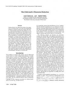
In this section we illustrate the operating characteristics of the likelihood ratio test of the hypothesis that ∆ is diagonal versus the general alternative, as described in Section 3.3. The data were generated according to the model Xy = Γy + ∆1/2 ε, √ with Y ∼ N (0, 1), Γ = (1, . . . , 1)T / p ∈ Rp and ε ∼ N (0, Ip ) where ∆ is a diagonal matrix with entry (i, i) equal to 10i−1 . For the fitted model we used the working dimension w = r, since inference on ∆ will likely be made prior to inference on d, and fy = (y, . . . , y r )T . Testing was done at the 5 percent level and the number of repetitions was 500. Figure 3.1 gives a graph of the fraction of runs in which the null hypothesis d = 1 was not rejected versus sample size for various values of r and two values of p. The results show, as expected, that the test performs well when n is large relative to p and r is not much larger than d. The test may be unreliable in other cases, particularly when there is substantial overfitting w = r À d. Bootstrap b y are a possible b βf b−Γ methods based on resampling the residual vectors Xy − µ alternative when n is not large relative to p.

3.7.2

Inference about d

Here we present some simulations about inference on d, using the likelihood ratio tests (LRT), AIC and BIC. We first generated Y ∼ N (0, σy2 ), and then with d = 2 generated Xy = Γβfy + ∆1/2 ε, where ε ∼ N (0, Ip ), β = I2 , fy = (y, |y|)T , √ and Γ = (Γ1 , Γ2 ) ∈ Rp×2 , with Γ1 = (1, 1, −1, −1, 0, 0, . . . , 0)T / 4 and Γ2 = √ (−1, 0, 1, 0, 1, 0, . . . , 0)T / 3. ∆ was generated as ∆ = AT A, where A is a p × p matrix of independent standard normal random variables, yielding predictor variances of about 10 and correlations ranging between 0.75 and -.67. The fitted model 41

1.0

1.0

0.8

0.8

r=1 r=3 r=6

0.6 0.4

F

r=5

r=10

0.2

0.2

0.4

F

0.6

r=1

0.0

0.0

r=15

50

100

150

200

50

n

100

150

200

n

a. p = 6

b. p = 15

Figure 3.1: Tests of a diagonal ∆: The x-axis represents sample size and the y-axis the fraction F of time the null hypothesis is not rejected

was PFC∆ with fy = (y, |y|, y 3 )T . Figures 3.2a-3.2d give the fraction F (2) of runs in which the indicated procedure selected d = 2 versus n for p = 5, four values of σy and the three methods under consideration. The number of repetitions was 500. As expected all three procedures improve with sample and signal (σy ) size. BIC and AIC get close to 100 percent and the likelihood ratio to 95 percent. In Figure 3.3 σy = 2 and n = 200. For Figures 3.3a and 3.3c, fy = (y, |y|, y 3 )T , while for the other two figures fy = (y, |y|, y 3 , . . . , y 10 )T . In Figures 3.3a and 3.3b the y-axis is the fraction of runs in which LRT, AIC or BIC chose the correct value d = 2. For Figure 3.3c y-axis is the fraction of runs in which d = 2 or 3 was chosen, and for Figure 3.3d the y-axis is the fraction of runs in which d = 2, 3 or 4 was chosen. Figures 3.3a and 3.3b show, as expected, that the chance of choosing the correct value of d decreases with p for all procedures. Figures 3.3c and 3.3d show that, with increasing p, LRT and AIC slightly overestimate d, while BIC underestimates d. In the case of AIC, we estimated nearly a 100 percent chance that the estimated d is 2, 3 or 4 with 80 predictors, r = 10 and 200 observations. A little overestimation

42

1.0

1.0

BIC LRT AIC

0.8

0.8

AIC

0.6

F(2) 0.4

0.4

F(2)

0.6

LRT

0.2 0.0

0.0

0.2

BIC

100

200

300

400

100

n

200

300

400

n

a. σy = .5

b. σy = 1

BIC

1.0

1.0

BIC

0.6

F(2) 0.4 0.2 0.0

0.0

0.2

0.4

F(2)

0.6

0.8

LRT AIC

0.8

LRT AIC

100

200

300

400

100

n

200

300

400

n

c. σy = 2

d. σy = 5

Figure 3.2: Inference about d, for d = 2 vs n: The x-axis is the sample size n. The y-axis is the fraction F (2) of runs in which d = 2 was chosen

seems quite tolerable in dimension reduction, and so we believe this to be a strong practical result. Based on these and other simulations we judged AIC and LRT are the best overall method for selecting d, although in the right situation either of the other methods may perform better. For instance, comparing the results in Figures 43

3.3a with the results in Figure 3.2c, we can see that for n = 200 and p = 5, the performance of BIC is better than AIC. Nevertheless that is reversed after p ∼ 10

1.0

1.0

where AIC consistently gives better results.

0.8

LRT

0.8

AIC

BIC

0.6

F(2)

F(2)

0.6

AIC

0.4

0.4

BIC

0.2 0.0

0.0

0.2

LRT

10

20

30

40

50

60

70

80

10

20

30

p

40

50

60

70

80

p

1.0

LRT

1.0

b. r = 10

AIC

0.8

a. r = 3

LRT

0.6

F(2,3,4)

0.4

0.6

BIC

0.2

0.4

BIC

0.0

0.0

0.2

F(2,3)

0.8

AIC

20

40

60

80

20

p

40

60

80

p

c. r = 3

d. r = 10

Figure 3.3: Inference about d: The x-axis is the number of predictors p. The y-axis for Figures a and b is the fraction F (2) of runs in which d = 2 was chosen; for Figure c it is the fraction F (2, 3) of runs where d = 2 or 3 was chosen; for Figure d it is the fraction F (2, 3, 4) of runs where d = 2, 3 or 4 was chosen.

44

3.7.3

Testing predictors

To study tests of Y

X2 |X1 , we generated data from the model Xy = Γy + ∆1/2 ε,

where ε ∼ N (0, Ip ) and Y ∼ N (0, σy2 ); ∆ was generated as in Section 3.7.2, and Γ = c(Γ1 , Γ2 )T ∈ R10 with Γ1 = (1, . . . , 1)T ∈ R7 , Γ2 = −∆−22 ∆21 Γ1 , and c is a normalizing constant. The fitted model was PFC∆ with d = r = 1 and fy = y. Partition X = (XT1 , XT2 )T with dim(X1 ) = 7. Shown in Figure 3.4 is the fraction of 500 runs in which the null hypothesis Y

X2 |X1 is not rejected at level α = 0.05 versus sample size for three values

of σy . Our general conclusion, as illustrated by the results in Figure 3.4, is that the actual and nominal levels of the test are usefully close for larger signals and reasonable sample sizes, but the test tends to reject too frequently for weak signals or small samples. We see that there is again a tendency for likelihood methods to overestimate, in this case the active predictors. As with inference on d we do not

1.0

judge this to be a serious issue in the context of this thesis.

σy = 3

0.9

σy = 1

0.5

0.6

0.7

F

0.8

σy = 0.5

50

100

150

200

250

300

n

Figure 3.4: Testing Y independent of X2 given X1 : The x-axis is the sample size and the y-axis is the fraction of runs in which the null hypothesis is not rejected.

45

3.7.4

Study of the Fearn’s data

Fearn’s (1983, see also Cook, 1998, p. 175) calibration data is the basis for this example. The response is the protein content of a sample of ground wheat, and the predictors are -log(reflectance) of NIR radiation at p = 6 wavelengths. The predictors are highly correlated in these data, with pairwise sample correlations ranging between 0.92 and 0.9991. Plots of each predictor versus Y suggest that fy = (y, y 2 , y 3 )T is a reasonable choice. Fitting model PFC∆ with this fy resulted in AIC, BIC and LRT all choosing d = 2. From the plot of those linear combinations versus the response it become clear that there is an strong linear relation between the first combination and the response and that there is an outlier point. Taking away that point from the analysis all three methods choose d = 1 which tells that the second combination is there just to be able to relate the response with the point in question. The linear regression of the response on the first linear combination gives an r2 = 0.9793 and the direction found forms a small angle with the ordinary least square slope. If we apply principal component to these data we need at least three components to get the same qualitative result and the principal components do not seem to have a clear relation with the response – this due to the fact that Σ = ∆ + Γvar(fy )Γ and therefore the relation we are interested in is the one given by the second term in the sum and without computing ∆ we are not able to get that term.

3.8

Conclusions

When using principal component methodology in the regression of Y on X, the ˆ jT X, j = predictors X are replaced by a few of the leading principal components v ˆ j is the eigenvector of 1, . . . , p, prior to regression with response Y ∈ R1 , where v b of X corresponding to its j-th largest eigenvalue the sample covariance matrix Σ ˆ1 > . . . > λ ˆ p . Such a use of principal components opens a discussion due to: λ

46

1) the fact the principal components are computed over the marginal distribution of the predictors without taking into account the response and therefore there is no theory behind that guarantees they are the only linear combinations needed for the regression of Y on X, and 2) they are not invariant under full rank linear transformations of the predictors, leading perhaps tolinear combinations for different scalings. In this chapter, beginning with an inverse model for the predictors X given the response Y with constant variance, the linear combinations of the predictors that are sufficient for the study of the regression of Y on X were obtained. The maximum likelihood estimator for these linear combinations are the first d principal b −1/2 X, with Σ b res = components based on the linearly transformed predictors Σ res b −Σ b fit and Σ b fit is the sample covariance matrix of the fitted vectors from the Σ multivariate linear regression of Xy on fy , including an intercept. These results provide remedies for two concerns that have dogged the use of principal components in regression: (i) principal components are computed from the predictors alone and do not make apparent use of the response, and (ii) principal components are not invariant under full rank linear transformation of the predictors. In addition, it was proved in this chapter that the SIR estimator under model PFC∆ with Y categorical is the maximum likelihood estimator of ∆−1 SΓ . This gives a clear connection between model PFC∆ and the model-free approach given by SIR.

47

Proofs of the results from Chapter 3 To be able to prove Theorem 3.1.1 we need three lemmas. Lemma 3.8.1 (Eaton, 1972, proposition 5.41) Consider the transformation  S=

 S11 S12 S21 S22



=

 V11

V11 V12

(V11 V12 )T

T V V V22 + V12 11 12



−1 + q1 ×q2 . Thus V where V11 ∈ S+ 11 = S11 , V12 = S11 S12 and q1 , V22 ∈ Sq2 and V12 ∈ R + + q1 ×q2 → S+ is 1-1 and onto. V22 = S22 − S21 S−1 p 11 S12 . The map g : Sq1 × Sq2 × R

A modification of the following lemma can be found on Anderson (1983) Theorem A.4.7. Lemma 3.8.2 Let A a diagonal positive definite matrix with eigenvalues 0 < a1 ≤ · · · ≤ ar and B a symmetric positive definite matrix with eigenvalues b1 ≥ · · · ≥ br > 0 and let H be a r × r orthogonal matrix. Then T

min trace(HBH A) = H

r X

ai bi .

i=1

If ai and bi are all different the minimum will occur only when H = Ir .

48

Lemma 3.8.3 Let S, J ∈ S0p and consider the partitions S = (Sij )i,j=1,2 , J = (Jij )i,j=1,2 , where S11 , J11 ∈ Sq1 with q1 ≤ p. Suppose J11 ∈ S+ q1 , J12 = 0 and J22 = 0, then the eigenvalues of S11 J11 are the same than the nonzero eigenvalues of SJ. Proof of Lemma 3.8.3: Let v be an eigenvector with eigenvalue λ 6= 0 of SJ. Let V1 be the first q1 rows of v. Then S11 J11 V1 = λV1 and S21 J11 V1 = λV2 . Thus, V1 is eigenvector of S11 J11 with eigenvalue λ. Proof of Theorem 3.1.1: In what follows f is used as a generic function whose definition changes and is given in context. We will make a series of changes of variables to rewrite the problem, the first one being S = D−1 . This transforms (5.10) into

p X

b res ) − f (S) = log |S| − trace(SΣ

b fit ). λi (SΣ

(3.9)

i=d+1

b 1/2 b 1/2 Now, let U = Σ res SΣres so that the problem becomes that of maximizing p X

f (U) = log |U| − trace(U) −

b −1/2 Σ b fit Σ b −1/2 ). λi (UΣ res res

(3.10)

i=d+1

b −1/2 b b −1/2 has rank τ = min(r, p) and is symmetric and positive semiSince Σ res Σfit Σres b −1/2 b b −1/2 = definite, we can use the singular value decomposition and write it as Σ res Σfit Σres b1 , . . . , λ bτ , 0, . . . , 0), bΛ bτV b T where V b ∈ Rp×p is an orthogonal matrix and Λ b τ = diag(λ V b1 > λ b2 > · · · > λ bτ > 0. Using this notation, (3.10) becomes with λ f (U) = log |U| − trace(U) −

τ X

bΛ b T ). bτ V λi (UV

i=d+1

b T UV b ∈ S+ , problem (5.10) is then equivalent to Using a new variable H = V p maximizing f (H) = log |H| − trace(H) −

τ X i=d+1

49

b τ ). λi (HΛ

(3.11)

+ We now partition H as H = (Hij )i,j=1,2 , with H11 ∈ S+ τ , H22 ∈ Sp−τ (for p = τ we

take H = H11 and go directly to (3.15)). Consider the transformation in Lemma + + τ ×(p−τ ) given by V 3.8.1 from S+ 11 = H11 , V22 = p to the space Sτ × Sp−τ × R −1 H22 − HT12 H−1 11 H12 and V12 = H11 H12 . This transformation is one to one and

onto. As a function of V11 , V22 and V12 , using Lemma 3.8.3, (3.11) can be written as f (V11 , V12 , V22 ) = log |V11 ||V22 | − trace(V11 ) − trace(V22 ) τ X T ˜ τ ), −trace(V12 V11 V12 ) − λi (V11 Λ

(3.12) (3.13)

i=d+1

b1 , . . . , λ bτ ). The term −trace(VT V11 V12 ) is the only one that ˜ τ = diag(λ where Λ 12 T V V depends on V12 . Since V11 is positive definite, V12 11 12 is positive semi-definite.

Thus, the maximum occurs when V12 = 0. This implies that H12 = 0, H11 = V11 and H22 = V22 ; therefore we can come back to the expression on H and our problem reduces to maximizing the function f (H11 , H22 ) = log |H11 | + log |H22 | − trace(H11 ) − trace(H22 ) −

τ X

˜τ) λi (H11 Λ

i=d+1

(3.14) This function is the sum of two parts, one involving only H11 , the other only H22 , that we can therefore maximize separately. The maximum of log |H22 | − trace(H22 ) is reached at H22 = Ip−τ . As for τ X

f (H11 ) = log |H11 | − trace(H11 ) −

˜ τ ), λi (H11 Λ

(3.15)

i=d+1

˜ 1/2 ˜ 1/2 leads us to maximize calling Z = Λ τ H11 Λτ ˜ −1 ) − f (Z) = log |Z| − trace(ZΛ τ

τ X i=d+1

50

λi (Z).

(3.16)

Since Z ∈ S+ τ , there exists an F = diag(f1 , . . . , fτ ) with fi > 0 in decreasing order and an orthogonal matrix W in Rτ ×τ such that Z = WT FW. As a function of W and F, (3.16) can be rewritten as τ X

˜ −1 ) − f (F, W) = log |F| − trace(WT FWΛ τ

fi = log |F|

i=d+1

˜ −1 WT ) − −trace(FWΛ τ

τ X

fi .

i=d+1

˜ −1 WT ) = Now, using a Lemma 3.8.2, minW trace(FWΛ τ

Pτ

b−1 i=1 fi λi ,

and if all the

c = Iτ . Knowing this, element of F and Λτ are different, the minimum occur when W we can rewrite the problem one last time, as that of maximizing in (f1 , . . . , fτ ), all greater than zero, the function f (f1 , . . . , fτ ) =

τ X

log fi −

i=1

τ X i=1

b−1 − fi λ i

τ X

fi .

(3.17)

i=d+1

bi for i = 1, . . . , d and for i = d + 1, . . . , τ , Clearly the maximum will occur at fi = λ bi /(λ bi + 1). Since λ bi are positive and decreasing order, fi are positive and fi = λ bi are different, the fi are different, Z b = F. b decreasing in order. Since all the λ

51

Collecting all the results, the value of D that maximizes (5.10) is b = S b −1 = Σ b 1/2 U b −1 Σ b 1/2 ∆ res res b 1/2 V bH b −1 V bTΣ b 1/2 = Σ res res   1/2 −1 ˜τ Z b Λ ˜ 1/2 Λ 0 τ τ ×(p−τ ) b 1/2 V b bTΣ b 1/2 V = Σ res res 0(p−τ )×τ Ip−τ ×(p−τ )    I 0 0 . . . d         0 λd+1 + 1 0  . . .    0τ ×(p−τ )    .   ... ..  . . . . . .  1/2  b V  = Σ res  . . . 0 0 λ + 1 τ      0(p−τ )×τ Ip−τ ×(p−τ ) 

        T b 1/2  V Σres      

 0d

   0  b res + Σ b 1/2 V  = Σ  ... res    0  0

0

0

...

λd+1

...

...

0 .. .

0

λτ

0

0

0

0p−τ ×(p−τ )

...

     T b 1/2  V Σres .    

b in the definition of Ld to Now, to obtained the maximum value we replace D by ∆ get, τ X b −1 Σ b n trace(∆ b −1 Σ b fit ). (3.18) b res )− n b = − np log(2π)− n log |∆|− λi (∆ Ld (∆) 2 2 2 2 i=d+1

52

Now, the trace and the eigenvalues are cyclic operations therefore −1

b trace(∆

b res ) = trace(∆ b −1/2 Σ b res ∆ b −1/2 ) Σ b p + K) b −1 V bT) = trace(V(I τ X bi ) + (p − τ ), = d+ 1/(1 + λ

(3.19) (3.20)

i=d+1

and τ X

b −1 Σ b fit ) = λi (∆

i=d+1

= = =

τ X i=d+1 τ X i=d+1 τ X i=d+1 τ X i=d+1

b + K) b −1 V bTΣ b −1/2 Σ b fit Σ b −1/2 ) λi (V(I res res bi (V(I b + K) b −1 V bTV bK bV bT) λ bi ((I + K) b −1 K) b λ bi λ bi 1+λ

.

(3.21) (3.22)

b res is an invertible operator we have Since Σ b = log |Σ b 1/2 V(I b + K) b V bTΣ b 1/2 | log |∆| res res b res ||V(I b + K) b V bT| = log |Σ τ X bi ). b res | + log(1 + λ = log |Σ i=d+1

53

(3.23) (3.24)

Plugging (3.19), (3.22) and (3.24) into (3.18) we get τ −1 np n n n X b b b b b −1 Σ b fit ) Ld (∆) = − log(2π) − log |∆| − trace(∆ Σres ) − λi (∆ 2 2 2 2 i=d+1

= −

n np b res | − n log(2π) − log |Σ 2 2 2

τ X

log(1 + λi ) −

i=d+1

n (p − τ + d) 2

τ τ n X n X 1 λi − − 2 1 + λi 2 1 + λi i=d+1

i=d+1

τ np n n X n n b = − log(2π) − log |Σres | − log(1 + λi ) − (p − τ + d) − (τ − d) 2 2 2 2 2 i=d+1

= −

τ X np np n b res | − n − log(2π) − log |Σ log(1 + λi ). 2 2 2 2 i=d+1

b = Σ b res + Proof of Corollary 3.1.1: Recall from Theorem 3.1.1 that ∆ b 1/2 b b b T b 1/2 b b −1/2 b b −1/2 Σ res VKV Σres . where V contains the eigenvectors of B = Σres Σfit Σres . The 1/2

b res AT )−1/2 AΣ b res transformation X → AX transforms B → B0 BBT0 , where B0 = (AΣ b is invariant, is an orthogonal matrix. Consequently, under the transformation K b → B0 V b and ∆ b → A∆A b T . The rest of the proof follows similarly. V To prove Corollary 3.1.2 we need a lemma. ˜ =Σ b −1/2 b 1/2 where M = (Ip + K) b −1 , with V b and K b as in Lemma 3.8.4 Let V res VM b 1/2 V ˜ are the normalized eigenvectors of ∆ b −1/2 Σ b fit ∆ b −1/2 Theorem 3.1.1. Then ∆ Proof of Lemma 3.8.4: From Theorem 3.1.1, b = Σ b res + Σ b 1/2 V bK bV bTΣ b 1/2 ∆ res res b 1/2 V(I b p + K) b V bTΣ b 1/2 . = Σ res res

54

Then, b −1 = Σ b −1/2 V(I b p + K) b −1 V bTΣ b −1/2 ∆ res res b −1/2 VM b V bTΣ b −1/2 . = Σ res res b are the eigenvectors of Σ b −1/2 b b −1/2 we get Using the fact that V res Σfit Σres b −1 Σ b fit V ˜ = Σ b −1/2 VM b V bTΣ b −1/2 Σ b fit Σ b −1/2 VM b 1/2 ∆ res res res 1/2 b −1/2 VM∆ b = Σ τM res

˜ 1/2 ∆τ M1/2 = VM ˜ = VM∆ τ b1 , . . . , λ bd , λ bd+1 /(λ bd+1 + 1), . . . , λ bτ /(λ bτ + 1), 0, . . . , 0). Therewhere M∆τ = diag(λ b1 , . . . , λ bd , λ bd+1 /(λ bd+1 + 1), . . . , λ bτ /(λ bτ + 1), 0, . . . , 0 b −1 Σ b fit has eigenvalues λ fore ∆ ˜ and with eigenvectors V, ˜T∆ bV ˜ = M1/2 V bTΣ b −1/2 ∆ bΣ b −1/2 VM b 1/2 V res res b T V(I b p + K) b V b T VM b 1/2 = M1/2 V = Ip . b 1/2 V ˜ are the normalized eigenvectors of ∆ b −1/2 Σ b fit ∆ b −1/2 Summarizing ∆ Proof of Corollary 3.1.2: As we said before the maximum likelihood estib −1/2 times the first d eigenvecmator for a basis of span(∆−1 Γ) is the span of ∆ b −1/2 Σ b fit ∆ b −1/2 . Now, from Lemma 3.8.4, span of the first d columns of tors of ∆ b −1/2 ∆ b 1/2 V ˜ = V ˜ is the maximum likelihood estimator for span(∆−1 Γ). Since ∆ b 1/2 and M is diagonal full rank with the first d elements equal 1, ˜ =Σ b −1/2 V res VM b ˜ is the same of the first d columns of Σ b −1/2 the span of the first d columns of V res V b b −1/2 b are the eigenvectors of Σ b −1/2 where V res Σfit Σres . This prove the fourth form of the expressions of the MLS of ∆−1 SΓ . The proof of the fifth form can be found in Cook 55

b −1 Σ b fit and Σ b −1 Σ b (2007a) and if follows from the fact that the eigenvectors of Σ res fit are bi and λ bi /(1 − λ bi ). The corollary follows identically, with corresponding eigenvalues λ now from the relation between the eigenvectors of the product of the symmetric 1

1

matrices AB and the eigenvectors of A 2 BA 2 . The second and the third forms of the expressions of the MLS of ∆−1 SΓ follow from the fourth and fifth forms and b =Σ b res + Σ b fit . and from the fact that Σ Proof of Lemma 3.5.1: Y true that Y

X2 |X1 if and only if Y

X|X1 . Suppose it is

X|X1 . We know that ΓT ∆−1 X is the minimal sufficient reductive

subspace for the regression of Y on X, thus ΓT ∆−1 X should not depend on X2 . Now,

 ΓT ∆−1 X = 

(ΓT1 ∆11 + ΓT2 ∆21 )X1 (ΓT1 ∆12 + ΓT2 ∆22 )X2

 

(3.25)

will not depend on X2 if and only if ΓT1 ∆12 + ΓT2 ∆22 = 0 equivalently Γ2 = −∆−22 ∆21 Γ1 . The reciprocal follows directly if we replace Γ2 by −∆−22 ∆21 Γ1 on equation (3.25). To prove Theorem 3.5.1 we need the following result Lemma 3.8.5 Proposition 5.21 (Eaton, 1972) Let  ∆=

 ∆11 ∆12



∆21 ∆22 be a p × p matrix where ∆ii is square for i = 1, 2. Let  ∆−1 = 

∆11 ∆12 ∆21 ∆22

Then, −1 ∆11 = (∆11 − ∆12 ∆−1 22 ∆21 ) −1 −1 ∆12 = −(∆11 − ∆12 ∆−1 22 ∆21 ) ∆12 ∆22 −1 ∆22 = (∆22 − ∆21 ∆−1 11 ∆12 )

56

 .

−1 −1 ∆21 = −(∆22 − ∆21 ∆−1 11 ∆12 ) ∆21 ∆11 .

Proof of Theorem 3.5.1: The function we need to maximize on G and D−1 is b + trace(D−1 PG(D−1 ) Σ b fit ). f (G, D−1 ) = log |D−1 | − trace(D−1 Σ) From the hypotheses on Γ, we have ΓT ∆−1 = (ΓT1 ∆11.2 , 0) where ∆11.2 = ∆11 − ∆12 ∆−22 ∆21 . Then ΓT ∆−1 Γ = ΓT1 ∆11.2 Γ1 . G1 will be the matrix form for the b 11,fit ) first p1 rows of G. For fixed D, trace(D11.2 G1 (G1 T D11.2 G1 )−1 G1 T D11.2 Σ as a function of G1 is maximized by choosing (D11.2 )1/2 G1 to be a basis for the b 11,fit (D11.2 )1/2 , yielding another partially span the first d eigenvectors of (D11.2 )1/2 Σ maximized log likelihood up to a constant −1

f (D

−1

) = log |D

−1 b

| − trace(D

Σ) +

d X

b 11,fit (D11.2 )1/2 ). λi ((D11.2 )1/2 Σ

(3.26)

i=1

Let us take the transformation from Lemma 3.8.1 defined by L11 = ∆11 −∆12 ∆−22 ∆21 , L22 = ∆22 and L12 = ∆12 ∆−22 . As a function of L11 , L22 , L12 we get b 22 + L22 LT Σ b f (L11 , L22 , L12 ) = log |L11 | + log |L22 | − trace(L22 Σ 12 12 ) b 21 ) b 11 + L12 L22 Σ −trace((L11 + L12 L22 LT12 )Σ +

d X

1/2 b 1/2 λi (L11 Σ 11,fit L11 )

i=1

Now, differentiating with respect to L12 in the last expression, we get that ∂f ∂L12 ∂2f ∂L212

b 12 L22 − 2Σ b 11 L12 L22 , = −2Σ b 11 ⊗ L22 . = −2Σ

∂f b −1 Σ b = 0 for L12 the maximum occurs when L12 = −Σ 11 12 . ∂L12 Replacing this in the last log likelihood function we get to the problem of maximizing

Therefore solving

57

on L11 and L22 the function b 22 ) − trace(L11 Σ b 11 ) (3.27) f (L11 , L22 ) = log |L11 | + log |L22 | − trace(L22 Σ b 12 Σ b −1 Σ b +trace(L22 Σ 11 12 ) +

d X

1/2 b 1/2 λi (L11 Σ 11,fit L11 ), (3.28)

i=1 −1

b Σ b since for L12 = −Σ 11 12 , −1

b 12 ) − trace(L12 L22 LT Σ b b b b −2trace(L22 LT12 Σ 12 11 ) = trace(L22 Σ12 Σ11 Σ12 ). b −1 so that we need to maximize on L11 The maximum on L22 is at L22 = Σ 22.1 b 11 ) + f (L11 ) = log |L11 | − trace(L11 Σ

d X

1/2 b 1/2 λi (L11 Σ 11,fit L11 ).

i=1

From Theorem 3.1.1 the maximum likelihood estimator for L11 will be such that b 1/2 b b b T b 1/2 L−1 11 = Σ11,res V(Id + K)V Σ11,res , bd+1 , . . . , λ bτ , 0, . . . , 0) and V b1 , . . . , λ bτ , 0, . . . , 0 the b = diag(0, . . . , 0, λ b and λ with K 1 1 b −1/2 Σ b b −1/2 eigenvectors and eigenvalues respectively of Σ 11,res 11,fit Σ11,res and τ1 = min(r, p1 ). Now, L11 = ∆11 − ∆12 ∆−22 ∆21 = ∆−1 11 and we get as the maximum likelihood estimator for ∆11 b 11 = Σ b 1/2 V(I b d + K) b V bTΣ b 1/2 , ∆ 11,res 11,res bd+1 , . . . , λ bτ , 0, . . . , 0) and V b1 , . . . , λ bτ , 0, . . . , 0 the b = diag(0, . . . , 0, λ b and λ with K 1 1 b −1/2 Σ b −1/2 b eigenvectors and eigenvalues respectively of Σ 11,res 11,fit Σ11,res . b −1 and −Σ b −1 Σ b b −1 The maximum likelihood estimators for ∆22 will be Σ 22.1 11 12 Σ22.1 for ∆12 . For the ∆ scale we get for ∆12 , b 11 Σ b −1 Σ b ∆12 = ∆ 11 12

58

and for ∆22 , −1

−1

b 22.1 + Σ b 21 Σ b ∆ b 11 Σ b Σ b ∆22 = Σ 11 11 12 . Now, the maximum likelihood estimator for a basis of ∆−1 Γ = (∆11.2 Γ1 , 0)T b −1/2 Σ b 11,fit ∆ b −1/2 Γ1 , 0)T with Γ1 the first d eigenvectors of ∆ b −1/2 . will be span (∆ 11 11 11 Using the same logic than in Corollary 3.1.1 it can be proved that the maximum b −1/2 Γ1 , 0)T , likelihood estimator for a base of span(∆−1 Γ) will in this case be (Σ 11,res b −1/2 Σ b b −1/2 with Γ1 the first d eigenvectors of Σ 11,res 11,fit Σ11,res . b res →P ∆ and Σ b fit →P Proof of Theorem 3.6.1: We only need to prove that Σ Γβvar(fY )β T ΓT . These two conditions follows as Proposition 4 of Cook (2007a). Requiring the errors to be uncorrelated but not necessarily normal, it is known that b →P Σ, and Σ Σ = var(X) = E(var(X|Y )) + var(E(X|Y )) = ∆ + Γβvar(fY )β T ΓT . b fit = XT PF X/n, we use PFC∆ model to write To find the limiting value of Σ ¯T XTy − X

¯ T + f T β T ΓT + ∆1/2 ε = µT − X y

and thus ¯ T ) + Fβ T ΓT + R∆1/2 , X = 1n (µT − X b fit PF X = Fβ T ΓT PF R∆1/2 , where R is the n × p matrix with rows εT . From this Σ contain four terms. The first of this is Γβ(Ft F/n)β T ΓT →P Γβvar(fY )β T ΓT . The b fit →P Γβvar(fY )β T ΓT . remaining terms contain F/n and goes to 0. Therefore we get Σ b =Σ b res + Σ b fit , take the difference of the limiting values for Σ b and Σ b fit to Since Σ b res . confirm the limiting value for Σ

59

3.8.1

Algorithm for ∆ with linear structure

We will maximize over those S = ∆−1 the function given in (3.9). To be able to do that we need first to compute the derivative of our function with respect to S b fit is symmetric we get without considering any structure. Because Σ r X ∂f (S) b res − b fit )uT (SΣ b fit )Σ b fit = S−1 − Σ vi (SΣ i ∂S i=d+1

where ui and vi indicate respectively the right and left eigenvectors corresponding b fit normalized so that v 0 uj = δij . Now, ∂S = Gh for any to the eigenvalue λi of SΣ i ∂sh b h = 1, . . . , m and using the change of rule, the fact that S and Σres are symmetric we get for each h = 1, . . . , m, r X ∂f (S) b fit ui (SΣ b fit )v T (SΣ b fit )Gh ) b res Gh ) − trace(Σ = trace(S−1 Gh ) − trace(Σ i ∂sh i=d+1

(3.29) where ui and vi indicate respectively the right and left eigenvectors corresponding b fit normalized so that v uj = δij . to the eigenvalue λi of SΣ i 0

b fit S1/2 = D−1/2 Σ b fit D−1/2 Now, let us denote by u ¯i the i−th eigenvector of S1/2 Σ corresponding to the λi eigenvalue (in decreasing order) normalized with unit norm. We get the relations a) ui = S1/2 u ¯i = D−1/2 u ¯i , b) vi = S−1/2 u ¯i = D1/2 u ¯i , c) b fit ui = λi D1/2 u Σ ¯i and d) vi0 uj = δij . We can rewrite (3.29) as r X ∂f (S) b res Gh ) − = trace(DGh ) − trace(Σ λi trace(D1/2 u ¯i u ¯Ti D1/2 Gh ) (3.30) ∂sh i=d+1

b fit D−1/2 . with λi and u ¯i eigenvalues and normalized eigenvectors of D−1/2 Σ ∂f (S) = 0 for h = To find the maximum likelihood estimator we need to solve ∂sh 1, . . . , m. In order to rewrite this equation in a pack way we introduce the vec operator. We denote vec of a matrix A ∈ Rq×r the vector of length q × r obtained by writing the columns of A one after another in a column. Using (3.30) we can

60

rewrite

∂f (S) = 0 for h = 1, . . . , m using the vec operator as ∂sh

b res ) + vec(Gh )T vec(Gh ) vec(D) = vec(Gh ) vec(Σ T

T

r X

λi vec(D1/2 u ¯i u ¯Ti D1/2 )

i=d+1

(3.31) ˜ = (vec(G1 ), . . . , vec(Gm )) and since D = for h = 1, . . . , m. Calling G

Pm

i=1 di Gi ,

˜ we can rewrite (3.31) as vec(D) = GD Ã ˜ T GD ˜ =G ˜T G

b res ) + vec(Σ

r X

! λi vec(D1/2 u ¯i u ¯Ti D1/2 )

(3.32)

i=d+1

˜ −1 G ˜ T vec(Σ b res ) (by one of the properties above ˜ T G) Now, if r = d we get D = (G ˜ T G) ˜ −1 exists) and S = D−1 = (Pm di Gi )−1 . The algorithm will be (G i=1 ˜ T G) ˜ −1 G ˜ T vec(Σ b res ) 1. Set D0 = (d01 , . . . , d0m ) = (G 2. Compute D0 =

Pm

0 i=1 di Gi

3. Compute S0 = D−1 0 4. Solve for n = 1, . . . , Ã ˜T

˜ Dn = (G G)

−1

˜T

G

b res ) + vec(Σ

r X i=d+1

61

! 1/2 Sn−1 Sn−1 T 1/2 S λi n−1 vec(Dn−1 u ¯i (¯ ui ) Dn−1 )

Chapter 4

Normal inverse models with constant variance: mean and variance connection In this chapter we will state and prove some results about model (2.4) (See Section 2.1.2): Xy = µ + Φθβfy + ∆1/2 ε ∆ = ΦΩΦT + Φ0 Ω0 ΦT0 . where fy ∈ Rr a known function of y with E(fY ) = 0 and β ∈ Rd×r has rank d ≤ min(r, p). SΦ = E∆ (SΓ ) and ε is normal with mean 0 and identity as covariance matrix. In Section 4.1 we consider different variations of model (2.4). In Section 4.2 we discuss the relation between the models we propose and several other dimension reduction methods. Estimation and related issues are discussed in Section 4.3. Our main points are supported by the simulations and illustrative analysis in Section 4.4 where we emphasize small sample behavior. Although we adopt a model-based 62

approach, this seems to be robust to a range of variation in the error distribution, as discussed in Section 4.3.5 and demonstrated in Section 4.4.

4.1

Variations within model (2.4)

In this section we briefly mention several fitting options within model (2.4), depending on the relationships between p, u, d and r. u = p: When u = p we can take Φ = Ip , Ω = ∆ and model (2.4) reduces to PFC∆ model, yielding Σ = ∆ + θβvar(fY )β T θ T . In this case, ∆ is an unstructured positive definite matrix. u = d: In this case, θ ∈ Ru×u is of full rank and we can define Θ = θβ ∈ Ru×r , resulting in the model Xy = µ + ΦΘfy + ε

(4.1)

∆ = ΦΩΦT + Φ0 Ω0 ΦT0 . This model, which has p + ur + p(p + 1)/2 parameters, can be used even if d < u in the population. This is equivalent to the extended PFC model introduced by Cook (2007a). Consequently we see that the extended PFC model in fact provides a upper bound SΦ on SY |X . d = r: If d = r then β ∈ Rd×d is of full rank and it can be absorbed into θ, resulting in a version of model (2.4) with Φ ∈ Rp×u , β = Id , and θ ∈ Ru×d which has rank d. u = p and d = min(p, r): As mentioned previously, when u = p we can take Φ = Ip , Ω = ∆ and model (2.4) reduces to PFC∆ model. Using the notation of

63

model (2.4), Xy = µ + θβfy + ε where now θ ∈ Rp×d and β ∈ Rd×r . If d = p = min(p, r) then we can take θ = Ip . If d = r = min(p, r) then β ∈ Rr ×r is full rank, and the product θβ ∈ Rp×r is an unconstrained rank r matrix. In either case, we arrive at a model of the form Xy = µ + βfy + ε,

(4.2)

which is the usual multivariate normal linear model for the regression of X on fy . For ease of later reference we will call this the full model. This model has p(r + 1) + p(p + 1)/2 real parameters.

4.2

Relationships with other methods

In the last section we mentioned how model (2.4) relates to the extended PFC model and to the usual multivariate normal linear model. Christensen (2007) developed relationships between model (2.4) with d = u and linear model theory. Model (2.4) is also closely related to several other models and methods. We describe some of those relationships in this section.

4.2.1

OLS and minimum discrepancy estimators

A connection between model (2.4) and OLS can be established by the following proposition. In preparation, let gy ∈ Rs denote a vector-valued function of y, and let Bg = Σ−1 cov(X, gY ) ∈ Rp×s , which is the matrix of population coefficients from the OLS multivariate linear regression of gY on X. Proposition 4.2.1 Assume model (2.4). Then span(Bg ) ⊆ span(ΦΩ−1 θ) = SY |X

64

(4.3)

with equality when rank{cov(fY , gY )} ≥ d. This proposition states that span(Bg ) is in fact contained in the central subspace, with equality for appropriate choices of gy . In particular, by using a flexible gy that has rank{cov(fY , gY )} ≥ d we can construct a consistent, albeit inefficient under model (2.4), estimator of the central subspace without knowing fy . Since this requirement on gy seems weak, it may partially explain the variety of available methods for estimation of SY |X . The minimum discrepancy approach of Cook and Ni (2005) allows one to turn b g of Bg into a model-free estimator of SY |X , assuming only the sample version B that span(Bg ) = SY |X and that the data are iid observations on (X, Y ) with finite fourth moments. This involves using a consistent estimator of the covariance ma√ b g ) − vec(Bg )} as the inner trix in the asymptotic normal distribution of n{vec(B product matrix in a quadratic discrepancy function. The resulting estimators make b g , but may be inefficient when model (2.4) holds to asymptotically efficient use of B a reasonable approximation. An instance of this development protocol was given by Cook and Ni (2006).

4.2.2

Seeded reductions and PLS

We use the following notation to incorporate partial least squares (PLS) and seeded p×q , and let C(v, a, A) reductions. Let A ∈ S+ p be positive definite, let a ∈ R

represent the projection, with respect to the A inner product, of A−1 a onto the A-invariant subspace K spanned by the columns of Kv (a, A) = (a, Aa, . . . , Av−1 a), where v is a positive integer; that is C(v, a, A) = PKv (A) A−1 a. When q = 1, K is called a cyclic invariant subspace or a Krylov subspace in numerical analysis. Cook, Li and Chiaromonte (2007) developed a model-free estimator of SY |X based on the sample version of the population object C(v, ν, Σ), where ν is a “seed matrix” with the property that Σ−1 Sν = SY |X . They show that dim[span{C(v, ν, Σ)}] = dim(SY |X ) for all v = 1, 2, . . ., and that there is a value v ∗ of v such that span{C(v ∗ , ν, Σ)} = 65

SY |X for all v ≥ v ∗ . The desired population object is then C(v ∗ , ν, Σ), where v ∗ needs to be estimated in practice along with Σ and ν. Choosing ν = cov(X, Y ) gives the population version of the basic PLS estimator, as introduced by Helland (1990). The effectiveness of PLS in many applications may be due in part to the fact that span[Kv∗ {cov(X, Y ), Σ}] is the smallest Σ-invariant subspace that contains cov(X, Y ). PLS can be viewed as an extension of OLS for forward linear regression that may be appropriate when dim(SY |X ) = 1 and p ≥ n, since it does not require inversion of Σ. Assume that rank{cov(fY , gY )} ≥ d. It then follows from Proposition 4.2.1 that cov(X, gY ) qualifies as a seed matrix. The proposition below shows a connection between seeded reductions and model (2.4). Proposition 4.2.2 Assume model (2.4). Then C{v, cov(X, gY ), Σ} = ΦC{v, cov(ΦT X, gY ), var(ΦT X)}.

(4.4)

When v ≥ v ∗ , the cyclic subspace for the right hand side equals SY |ΦT X = Ω−1 Sθ , while the cyclic subspace for the left hand side equals SY |X . Thus, represented in terms of central subspaces, we again have SY |X = ΦSY |ΦT X (cf. Proposition 2.1.4). In summary, under model (2.4), the family of moment estimators represented by (4.4) includes PLS as a special case and seems to cover all of the known seed matrices. It bypasses direct estimation of the upper bound SΦ , and instead simultaneously estimates SY |ΦT X and transforms it with Φ to yield an estimate of SY |X . The estimators in this family do not require inversion of Σ, which is an advantage in applications where the sample size n is not large relative to p. However, while these estimators do extract information from the marginal distribution of X, they do not make full use of the information provided by the likelihood for (2.4) and thus may be inefficient in some regressions.

66

4.2.3

Discriminant analysis

As it was describe in Section 3.2.3, the condition that X and Y have a joint distribution allows a reduction based on inverse regression X|Y to be passed to the forward regression Y |X. However, when the inverse regression X|Y is itself the goal, this distributional requirement is unnecessary, as in discriminant analysis. Consider as a special case classifying a new observation Xnew into one of two normal populations C1 and C2 with means µ1 and µ2 and common covariance matrix ∆. Assuming equal prior probabilities, the optimal rule (Seber, 1984, p. 331) is to classify Xnew as arising from C1 if (µ1 − µ2 )T ∆−1 Xnew > (µ1 − µ2 )T ∆−1 (µ1 + µ2 )/2. As we describe in Chapter 3, this setting is described by PFC∆ model with r = 1, fy = J(y ∈ C1 ) and sufficient reduction SY |X = ∆−1 span(µ1 − µ2 ). Here, J(·) denotes an indicator function. Consequently, using the optimal rule in conjunction with PFC∆ model leads to Fisher’s classification rule for two normal populations. Proceeding similarly under model (2.4), the optimal rule is to classify into C1 if (µ1 − µ2 )T ΦΩ−1 ΦT Xnew > (µ1 − µ2 )T ΦΩ−1 ΦT (µ1 + µ2 )/2. Since µ1 − µ2 = Φθβ, where now β ∈ R1 , this rule can be expressed equivalently as θ T Ω−1 ΦT Xnew > θ T Ω−1 ΦT (µ1 + µ2 )/2, where we have assumed that β > 0 without loss of generality. When u ¿ p we can expect misclassification rates for this rule to be substantially lower than those for the standard rule based on PFC∆ model. In cases where d = u = 1, span(µ1 −µ2 ) = SΦ and the rule simplifies to (µ1 − µ2 )T Xnew > (µ1 − µ2 )T (µ1 + µ2 )/2.

67

4.3

Estimation

In this section we discuss maximum likelihood estimation and inference procedures.

4.3.1

MLE under model (2.4)

Estimation of the parameters in model (2.4) is facilitated by centering as in the ¯ The transformed vectors ΦT X and PFC∆ model so that again the MLE of µ is X. ΦT0 X are independent, with covariance matrices Ω and Ω0 , and thus the likelihood factors in these quantities. This leads to the log likelihood maximized over φ L(Φ, θ, β, Ω0 , Ω|d, u) = L0 + L1 (Φ0 , Ω0 |u) + L2 (Φ, θ, β, Ω|d, u) where L0 = −(np/2) log(2π), L1 (Φ0 , Ω0 |u) = − (n/2) log |Ω0 | − (1/2)

n X

¯ T Ω−1 ΦT (Xi − X) ¯ {ΦT0 (Xi − X)} 0 0

i=1

L2 (Φ, θ, β, Ω|d, u) = − (n/2) log |Ω| − (1/2)

n X ¯ − θβ(fi − ¯f )}T Ω−1 {ΦT (Xi − X) i=1

¯ − θβ(fi − ¯f )}. {Φ (Xi − X) T

e 0 = ΦT ΣΦ b 0 . Substituting back, we It follows that L1 is maximized over Ω0 by Ω 0 find the following partially maximized form for L1 : b 0 | − n(p − u)/2. L1 (Φ0 |u) = −(n/2) log |ΦT0 ΣΦ

(4.5)

For fixed Φ, the log likelihood summand L2 is in the same form as the likelihood considered for the PFC∆ model in Section 3.1, with the parameters and variables ¯ → ΦT (Xy − X). ¯ Thus for fixed redefined as ∆ → Ω, p → u, Γ → θ and (Xy − X)

68

Φ we have from (3.5) a partially maximized version of L2 : min(u,r)

b res Φ| + L2 (Φ|d, u) = −(n/2)[u + log |Φ Σ T

X

log{1 + vj (Φ)}],

j=d+1

where vj (Φ) indicates the j-th eigenvalue of b res Φ)−1/2 (ΦT Σ b fit Φ)(ΦT Σ b res Φ)−1/2 ∈ Ru×u , (ΦT Σ with corresponding eigenvectors given by the columns of V(Φ). The last summand on the right is 0 if d = u. Combining the three terms in L we have the partially maximized form L(Φ|d, u) = −(np/2){1 + log(2π)} −

n b 0 | + log |ΦT Σ b res Φ| [log |ΦT0 ΣΦ 2

min(u,r)

+

X

log{1 + vj (Φ)}]

j=d+1

= −(np/2){1 + log(2π)} − +

d X

n b 0 | + log |ΦT ΣΦ| b [log |ΦT0 ΣΦ 2

log{1 + vj (Φ)}]

j=1

n b −1 Φ| + log |ΦT Σ b res Φ| [log |ΦT Σ 2 min(u,r) X log{1 + vj (Φ)}], +

= C−

(4.6) (4.7)

j=d+1

b The form (4.7) shows that inforwhere C = −(np/2){1 + log(2π)} − (n/2) log |Σ|. b res and Σ b −1 . Evidently arg max L(Φ|d, u) does not have mation on Φ comes from Σ a closed-form solution and must be determined by maximization over G(u,p) . b has been determined, equations (3.4), (3.6) and (3.7) can be used to Once Φ

69

determine the MLEs of the remaining parameters: b0 = Φ bTΣ bb Ω 0 Φ0 b = (Φ bTΣ b res Φ) b 1/2 V(I b u+D b d,u )V b T (Φ bTΣ b res Φ) b 1/2 Ω b = (Φ bV b d )−1/2 b d (V bTΦ b res Φ bTΣ b res Φ) b 1/2 V bTΣ θ d b = (V bTΦ bTΣ b res Φ bV b d )1/2 V b T (Φ bTΣ b res Φ) b −1/2 Φ bTB bf, β d d b f ∈ Rp×r denote the estimated coefficient matrix from the OLS fit of Xi on where B b d,u = diag{0, . . . , 0, vd+1 (Φ), b . . . , vu (Φ)} b and V b d is the matrix consisting of fi and D b = V(Φ). b The sufficient reduction is thus estimated as the first d columns of V b T (Φ bTΣ b res Φ) b −1/2 Φ b T X. b R(X) =V d

4.3.2

(4.8)

MLE under model (4.1)

The MLE of SΦ under model (4.1) is obtained by maximizing over G(u,p) the partially maximized log likelihood −1

b L(Φ|u) = C − (n/2)(log |ΦT Σ

b res Φ|), Φ| + log |ΦT Σ

(4.9)

where C is as defined for (4.7). This log likelihood is equivalent to that given by b is obtained, the MLE’s for the remaining parameters Cook (2007a). Once a basis Φ can be obtained by setting d = u in the MLE’s of Section 4.3.1 and noting that, T

b u is an orthogonal matrix and D b u,u = 0. We thus have Ω b0 = Φ b Σ bb with d = u, V 0 Φ0 , b = Φ bTΣ b res Φ b and Θ b = Φ bTB b f , and we can estimate a sufficient reduction as Ω b T X. b R(X) =Φ

4.3.3

Choosing d and u

The dimensions d and u of SY |X and SΦ were so far assumed known. There are several ways in which these dimensions can be chosen in practice. It will be helpful 70

in this section to distinguish the true values (d, u) from values (d0 , u0 ) used in fitting. A joint hypothesis d = d0 , u = u0 can be tested by using the likelihood ratio statistic Λ(d0 , u0 ) = 2{Lfull − L(d0 , u0 )}, where Lfull denotes the value of the maxb 0 , u0 ) is the imized log likelihood for the full model (4.2) and L(d0 , u0 ) = L(Φ|d maximum value of the log likelihood (4.7) for model (2.4). Under the null hypothesis Λ(d0 , u0 ) is distributed asymptotically as a chi-squared random variable with r(p−d0 )−d0 (u0 −d0 ) degrees of freedom. When there is only one dimension involved it is standard practice to use a sequence of hypothesis tests to aid in its selection. However, in this case there seems no natural way to order the pairs (d0 , u0 ) for a sequence of such tests. One way to proceed is to compare model (4.1) to the full model b 0) using the likelihood ratio statistic Λ(u0 ) = 2{Lfull − L(u0 )}, where L(u0 ) = L(Φ|u is the maximum value of (4.9). Under the null hypothesis Λ(u0 ) has an asymptotic chi-squared distribution with r(p − u0 ) degrees of freedom. Testing is done sequentially, starting with u0 = 0 and estimating u as the first hypothesized value that is not rejected. Having chosen an estimate u b, d can be estimated similarly treating u b as known and using the likelihood ratio statistic Λ(d0 , u b) for 0 ≤ d0 ≤ u b. This method is inconsistent since there is a positive probability that the estimates of d and u will exceed their population values asymptotically. This probability depends on the levels of the tests. We do not regard mild overestimation of d or u as a serious issue and, in any event, overestimation in this context is a lesser problem than underestimation. We therefore believe that this procedure may have value in practice. The second approach is to use an information criterion like AIC or BIC. BIC is consistent while AIC is minimax-rate optimal (Burnham and Anderson, 2002). For 0 ≤ d0 ≤ u0 ≤ p, the dimensions are selected to minimize the information criterion IC(d0 , u0 ) = −2 L(d0 , u0 ) + h(n)g(d0 , u0 ), where g(d0 , u0 ) = p + d0 (u0 + r − d0 ) + p(p + 1)/2 is the number of parameters to be estimated as a function of (d0 , u0 ), and h(n) is equal to log n for BIC and 2 for AIC.

71

4.3.4

Prediction

Given a new observation Xnew on X, there are two general ways in which we might construct a prediction yb of the corresponding Ynew . One way is to develop a forb and then predict Ynew in the context of that model. ward regression model for Y |R However, it is not necessary to develop a forward model for prediction purposes. Let N (·|y) denote the normal density of X|Y under model (2.4). Perhaps the most common prediction method from a forward regression Y |X is to use the conditional mean E(Y |Xnew ) =

E{Y f (Xnew |Y )} . E{f (Xnew |Y )}

A straightforward estimator of E(Y |Xnew ) that does not require the development of a forward model is

Pn

b (Xnew |Y = yi ) yi N yb = Pi=1 , n b i=1 N (Xnew |Y = yi )

(4.10)

b denotes the estimated density of X|Y . Predicting Y for each value Xi of X where N in the data gives residuals yi − ybi , i = 1, . . . , n, that can use to diagnose deficiencies in the forward model that is implied by the inverse model. A common method when Y is categorical is to predict the category that maximizes Pr(Y = y|Xnew ) = N (Xnew |Y = y) Pr(Y = y)/E{N (Xnew |Y )}. Since the denominator plays no role in the maximization, we have, substituting estimates, b (Xnew |Y = y)Pr(Y c yb = arg max N = y), y∈SY

(4.11)

c c where Pr(Y = y) is an estimated or prior mass function for Y . If Pr(y) places equal

72

mass at each category in SY then b (Xnew |Y = y) yb = arg min N y

T

−1

bβ(f b y − ¯f )}T Ω b (Xnew − X) ¯ −θ b = arg min{Φ y

T

bβ(f b y − ¯f )} b (Xnew − X) ¯ −θ {Φ (4.12)

For example, suppose that Y is categorical with h equally likely categories, so that bβ b=B b = Ip , and θ b f . In this case the r = h − 1, u = p and d = min(p, r). Then Φ prediction reduces to the usual rule for normal classification: ¯ y }T Ω b −1 {Xnew − X ¯ y} yb = arg min{Xnew − X y

¯ y is the mean in class y ∈ {1, . . . , h}. where X

4.3.5

Robustness

Consider relaxing the assumption that the errors in model (2.4) are normally distributed while maintaining all other structure. In this section we show that the log likelihood (4.7) produces a Fisher consistent estimator of SΦ without imposing normality. Consequently, the estimation methods proposed here might be expected to furnish useful results as long as the moment structure of model (2.4) holds to a reasonable approximation. To avoid notational confusion, we replace Φ in (4.7) with the generic argument F. Then neglecting constants and multiplying by 2/n, the kernel of the log likelihood converges in probability to ˜ L(F|d, u) = −[log |FT0 ΣF0 | + log |FT ∆F| +

u X

log{1 + vj (F)}],

j=d+1

where vj (F) indicates the j-th eigenvalue of (FT ∆F)−1/2 (FT Σfit F)(FT ∆F)−1/2 , Σfit = Φθβvar(fY )β T θ T ΦT , and Σ is ΣΦ{Ω + θβvar(fY )β T θ T }ΦT + Φ0 Ω0 ΦT0 . 73

˜ Since Σfit has rank d, vj (F) = 0 for j ≥ d + 1, and consequently L(F|d, u) = − log |FT0 ΣF0 |−log |FT ∆F|. The desired conclusion then follows from Cook (2007a, prop. 5).

4.4

Simulations and data analysis illustrations

As discussed in Section 4.2, the proposed methodology can be adapted to many different contexts, each with its own considerations. In this section we illustrate methodological potential in discriminant analysis, a context that is important in its own right, and in graphical exploration. The discussion in the next section is limited to discrimination of two classes, since that context is sufficiently rich to allow illustration of our main points.

4.4.1

Discriminant analysis

As discussed in Section 4.2.3, when Y is a binary indicator, r = 1, fy = J(y ∈ C1 ) and SY |X = ∆−1 span(µ1 − µ2 ). We suppose it is known that µ1 6= µ2 and consequently d = 1. With these settings we generated multivariate normal observations from model (2.4) with p = 10 predictors and selected values for the remaining parameters. For each data set the log likelihood (4.7) was maximized using a program for optimization over Grassmann manifolds developed using the results of Edelman et al. (1999) and Liu et al. (2004) (For the implementation we followed Cook, 2007b). We chose u b using the likelihood testing method discussed in Section 4.3.3 at constant level 0.01. The remaining parameters were estimated using the likelihood estimators described in Section 4.3.1. The empirical model was evaluated by classifying 100 new observations from each of the two parent populations and computing the percentage of correct classifications. The number of replications was 400. Figure 4.1a shows the average percentage of correct classifications for u = 1, Ω = 16, Ω0 = I9 , Φ a 10 × 1 vector of 0’s with a 1 in the last position, and n/2 74

90

100

φ

85 70 65

60

80

Correct Classifications

80 70

u φ

LDA

^ u

75

90

LDA

50

Percentage of correct classifications

^ u

0

5

10

15

20

0

20

δ

40

60

80

δ

a. δ = kµ1 − µ2 k

b. Sample size, n

Figure 4.1: Percentage of correct classifications versus the indicated variable.

samples from each population. This corresponds to generating the first 9 predictors (features) as independent N (0, 1) variate, and generating the 10-th predictor as N (0, 16) in one population and N (δ, 16) in the other, where δ = kµ1 −µ2 k = kΦθβk. Figure 4.1a gives the average percentage of correct classification as a function of δ with n = 18. The upper line, labeled Φ, corresponds to the classification rule in which Φ is known, so only µ1 − µ2 needed to be estimated. The corresponding line for the optimal population classification percentages (not shown) lies uniformly above the Φ line, but the maximum observed difference was only 0.97 percent. Consequently, it is impossible for any method to do notably better than the bound represented by Φ. The second line, labeled u, is for the estimator with u = 1 known. The third line, identified by individual plotted points, gives the results when u b was chosen with likelihood testing, and the final line gives the results for Fisher’s linear discriminant (LDA). Except for small δ, the u b curve dominates linear discrimination and is relatively close to the reference simulations identified by the Φ and u lines. Evidently, there is relatively little cost to choosing u by likelihood testing, while the cost of ignoring the structure of ∆ can be substantial. Figure 4.1b shows the average percentage of correct classifications versus n for δ = 10, starting with n = 14. This illustrates a general observation that classification 75

rates based on model (2.4) can respond much faster to increasing sample size than LDA. The behavior of the curves for small n can be explained by examining the empirical distribution of u b. For n = (14, 20, 50), u b overestimated u = 1 about (40, 15, 4) percent of the time. Likelihood testing rejects too frequently relative to the nominal rate when n is small, which explains the results for n = 14 and n = 18 and leads to overestimation of u. While further improvements for small samples might be possible by pursuing the “best” method for choosing u, on balance some overestimation does not seem to be a worrisome issue. Recall from Section 4.3.5 that estimators under model (2.4) can be expected to exhibit some level of robustness to the error distribution. Shown in Table 4.1 are results from simulations constructed according to those of Figure 4.1b with n = 18, but under four different error distributions, each normalized to have mean 0 and variance 1. The first three rows give the percentage of correct classifications under the indicated method and error distribution. The fourth row gives the percentage of runs in which u b = 1 and u b = 2. Changing the error distribution does not seem to caused change for the estimation of u and for the estimation of classification. Table 4.1: Simulation results with alternative error distributions Method Φ u b LDA u b = (1, 2)

N (0, 1) 88.72 85.53 75.75 (84, 15)

Error distribution t5 U (0, 1) χ25 90.94 86.14 91.27 86.52 82.05 87.65 76.82 74.23 76.32 (80, 18) (79, 19) (84, 19)

As a second illustration we considered the problem of predicting the presence of a Pea Crab living inside a mussel shell based on the logarithms of six measurements: shell length, width and height, and shell, muscle and viscera masses. There are 172 cases of which 111 are mussels containing a Pea Crab. For these data u b = 1 and consequently we might expect notable differences between the methods notwith76

0.30 0.25

0.4

0.10

0.15

Density

0.20

0.3 0.2

Density

0.00

0.05

0.1 0.0 −4

−2

0

2

4

−4

^ L1

−2

0

2

4

^ R1

a. LDA

b. Model (2.4)

b 1 and R b1 with separate Figure 4.2: Pea Crab data: Plots of the first LDA variate L density estimates for mussels with a Pea Crab (right density) and for mussels without a Pea Crab (left density).

standing the fairly large sample size. Figure 4.2 shows Gaussian conditional density estimates with tuning parameter 0.8 for the LDA and model (2.4) classifiers, against a background histogram of the full data. It seems clear that the classifiers behave quite differently, and that the classification score estimated with model (2.4) affords a better separation than the LDA score.

4.4.2

Graphical exploration

We use data from the Australian Institute of Sport to illustrate the use of reductions in graphical exploration. The response Y is an athlete’s lean body mass (LBM) and the 8 predictors include 5 hematological measures – plasma ferritin concentration, Hematocrit, Hemoglobin, red cell count and white cell count – in addition to height, weight and sum of skin folds. The log scale was used for all predictors. We began by inspecting scatterplots of each predictor against the response, concluding that fyT = (y, y 2 , y 3 ) would be sufficient to describe the conditional means E(Xj |Y ). We inferred u b = 5 using model (4.1) and sequential likelihood testing with level 0.01. We next used model (2.4) with u fixed at 5 to infer about d in a

77

120 100

100

60

LBM

80

80 LBM

40

60

20

40

230

240

250

260

270

280

−11

^ R1

−10

−9

−8

−7

−6

^ R2

a. First sufficient reduction

b. Second sufficient reduction

b1 and R b2 for the data Figure 4.3: Plots of the first two estimated reductions R from the Australian Institute of Sport. The curves are lowess smooths with tuning parameter 0.6.

similar fashion, obtaining dˆ = 2. In other words, the minimal sufficient reduction was inferred to be two dimensional; R = (R1 , R2 )T . As a check, the likelihood ratio test failed to reject the joint hypothesis u = 5, d = 2, still using level 0.01. b1 and R b2 . FigFigures 4.3a,b give plots of the response versus the estimates R ure 4.3a shows a strong linear trend with evidence of curvature in the first direction, and Figure 4.3b shows a cubic trend. At this point there are several options available, depending on the specific goals of the analysis. For instance, a forward model might be developed using Figure 4.3 as a guide. Or we might proceed directly to prediction using (4.10).

4.5

Discussion

We cannot expect much progress to result from the use of elaborate models and methods when there are many parameters and the sample size is small. The main point of our paper is that parsimonious parameterization of the variance through the use of envelopes and the use of maximum likelihood estimation produces a new class of efficient and sufficient dimension reduction methods that seem to perform 78

well in small samples.

79

Proofs of the results from Chapter 4 Proposition 4.5.1 Let M ∈ Sp×p , let S ⊆ span(M), and let Pi be the projection P onto the i-th eigenspace of M, i = 1, . . . , q. Then EM (S) = qi=1 Pi S. This proposition, which follows from Proposition 4.5.2 and the definition of envelopes, gives an alternative characterization of an M-envelope. It states that EM (S) can be represented as the sum of subspaces obtained by projecting S onto the eigenspaces of M. Proposition 4.5.2 Let M ∈ Sp×p . If R reduces M then M has eigenvectors in R P or in R⊥ . Further, R reduces M if and only if R = qi=1 Pi R, where Pi is the projection onto the i-th eigenspace of M. Proof of Proposition 4.5.2: Let A0 ∈ Rp×u be a semi-orthogonal matrix whose columns span R and let A1 be its completion, such that (A0 , A1 ) ≡ A is an orthogonal matrix. Because MR ⊆ R and MR⊥ ⊆ R⊥ , it follows from Lemma 2.4.1 there exist matrices B0 ∈ Ru×u and B1 ∈ R(p−u)×(p−u) such that MA0 = A0 B0 and MA1 = A1 B1 . Hence     ³ ´ ³ ´ B0 0 B0 0  ⇔ M = A  AT . M A0 A1 = A0 A1  0 B1 0 B1

80

Because M is symmetric, so must be B0 and B1 . Hence B0 and B1 have spectral decompositions C0 Λ0 CT0 and C1 Λ1 CT1 for some diagonal matrices Λ0 and Λ1 and orthogonal matrices C0 and C1 . Let C = diag(C0 , C1 ) and Λ = diag(Λ0 , Λ1 ). Then, M = ACΛCT AT ≡ DΛDT ,

(4.13)

where D = AC. The first u columns of D, which form the matrix A0 C0 , span R. Moreover, D is an orthogonal matrix, and thus (4.13) is a spectral decomposition of M with eigenvectors in R or R⊥ . To show the second part of the proposition, assume that R reduces M. If v ∈ R, then à v = Ip v =

q X

! Pi

v=

i=1

Hence R ⊆

Pq

i=1 Pi R.

q X

Pi v ∈

i=1

Conversely, if v ∈

Pq

i=1 Pi R,

q X

Pi R.

i=1

then v can be written as a

linear combination of P1 v1 , . . . , Pq vq where v1 , . . . , vq belong to R. By the first part of this proposition, Pi w ∈ R for any w ∈ R. Hence any linear combination of P P1 v1 , . . . , Pq vq , with v1 , . . . , vq belonging to R, belongs to R. That is, qi=1 Pi R ⊆ Pq R. This proves that if R reduces M then R = i=1 Pi R. Next, assume that Pq Pq R = i=1 Pi R. Then for any vectors v1 , . . . , vq in R, i=1 Pi vi ∈ R. In particular, choosing all vectors except one equal to the zero vector we have Pi v ∈ R for any v ∈ R, i = 1, . . . , q. Therefore, for any v ∈ R, Mv ∈ R. Proof of Proposition 4.2.1: Let M = ∆ + θβvar(fY )β T θ T . Then under model (2.4) it can be verified that Σ = E(var(X|Y )) + var(E(X|Y )), = ΦMΦT + Φ0 Ω0 ΦT0 , T Σ−1 = ΦM−1 ΦT + Φ0 Ω−1 0 Φ0 ,

81

ΣΦ = ΦM, ΦT ΣΦ = M and cov(X, gY ) = Φθβcov(fY , gY ). It follow from these relationships that Bg = Σ−1 cov(X, gY ) T = (ΦM−1 ΦT + Φ0 Ω−1 0 Φ0 )Φθβcov(fY , gY )

= Φ(ΦT ΣΦ)−1 ΦT ΣΣ−1 Φθβcov(fY , gY ) = PΦ(Σ) Bg PΦ(Σ) = Φ(ΦT ΣΦ)−1 ΦT Σ = ΦM−1 MΦT = PΦ Bg = PΦ Bg = ΦM−1 αcov(fY , gY ) where α = θβ for notational convenience. Now, letting V = var(fY ), M−1 = (Ω + αVα)−1 = Ω−1 − Ω−1 α(V−1 + αT Ω−1 α)−1 αT Ω−1 ΦM−1 α = ΦΩ−1 α − ΦΩ−1 α(V−1 + αT Ω−1 α)−1 αT Ω−1 α = ΦΩ−1 α(Ir − (V−1 + αT Ω−1 α)−1 αT Ω−1 α) = ΦΩ−1 α(V−1 + αT Ω−1 α)−1 V−1 = ΦΩ−1 α(V(V−1 + αT Ω−1 α))−1 = ΦΩ−1 α(Ir + VαT Ω−1 α)−1 Consequently, Bg = ΦΩ−1 α(Ir + VαT Ω−1 α)−1 cov(fY , gY ) and span(Bg ) = span(ΦΩ−1 θ) if β(Ir +VαT Ω−1 α)−1 cov(fY , gY ) has rank d. Since β has rank d, this will be so if the rank of cov(fY , gY ) is at least d.

82

Proof of Proposition 4.2.2: To prove this proposition use the following relationships. cov(X, gY ) = Φθβcov(fY , gY ) ∈ Rp×s cov(ΦT X, gY ) = θβcov(fY , gY ) Σr = ΦMr ΦT + Φ0 Ωr0 Φ0 ΦT Σr Φ = Mr where M is as defined in the proof of Proposition 4.2.1. Therefore Σr cov(X, gY ) = ΦMr θβcov(fY , gY ) Kv {cov(X, gY ), Σ} = ΦKv {cov(ΦT X, gY ), var(ΦT X)} ∈ Ru×s(v −1 ) For notational convenience let Kv = Kv {cov(X, gY ), Σ} and K∗v = Kv {cov(ΦT X, gY ), var(ΦT X)}. Then C{v, cov(X, gY ), Σ} = Kv (KTv ΣKv )−1 KTv cov(X, gY ) T ∗ −1 ∗T T = ΦK∗v (K∗T v Φ ΣΦKv ) Kv cov(Φ X, gY )

= ΦC{v, cov(ΦT X, gY ), var(ΦT X)}.

83

Chapter 5

Normal inverse models with non-constant variance In this chapter we will state and prove some results about model (2.8): Xy = µ + ∆αν y + ∆1/2 y ε.

(5.1)

with ε normally distributed with mean 0 and covariance matrix identity and 1. µy = µ + ∆αν y with E(ν Y ) = 0. 2. ∆y = ∆ + ∆αTy αT ∆, with E(TY ) = 0. The goal is to estimate the central subspace, Sα . To do that we will assume that the data consist of ng independent observations Xg ∈ Rp for each g = 1, . . . , h where g represent the population g or g represent the observations on each slices if Y is continuous and we sliced. In generality, slicing the range of Y is done by partitioning the range of Y into h slices or bins Hk and then replacing Y by k when Y ∈ Hk . Under this setting, in this chapter we derive the maximum likelihood estimator for Sα , the central subspace. In Section 5.1 we give the MLEs under model (5.1). In Section 5.2 we study inference about the dimension of the central 84

subspace. Testing variables is done in Section 5.3. We compare our method with SIR and SAVE methodology in Section 5.4. Finally in Section 5.5 we illustrate our method in a data set where the goal is to distingue among birds, planes and cars. We show in this example how our method performs better than SIR, SAVE and the recently presented method, Direction Reduction (DR; Li and Wang, 2007).

5.1

Estimation of Sα when d is known

From Proposition 2.2.2 the minimal linear sufficient reduction is of the form R = αT X. Following Proposition 3.2 from Shapiro (1986) the analytic dimension of the full parameter space (∆g , ∆, α, µ) for model (2.8) is equal to the rank of the Jacobian of the parameters and is equal p + (h − 1)d + p(p + 1)/2 + d(p − d) + (h − 1)d(d + 1)/2 for almost all points in the parameter space (a proof can be found in http://liliana.forzani.googlepages.com/degrees07122007.pdf). The following theorem summarizes maximum likelihood estimation when d = dim Sα is specified. We assume the data consist of ng independent observations of Xg ∈ Rp , g = 1, . . . , h. ˜ indicate sample moments and Σ b indicate MLE estimators. In this chapter Σ Theorem 5.1.1 Under model (2.8) the maximum likelihood estimator for Sα is the b ∈ Rp×d that maximizes over SB ∈ G(d,p) the log span of any semi-orthogonal basis α likelihood function Ld (SB ) = −

X np n ˜ − n log |Σ| ˜ −1 ˜ g B| (1 + log(2π)) + log |BT ΣB| ng log |BT ∆ 2 2 2 2 g (5.2)

where B ∈ Rp×d is a semi-orthogonal matrix whose columns form a basis for SB , ˜ is the marginal covariance matrix of X and ∆ ˜ g is the covariance matrix for Σ b of ∆ the data belonging to population g. The maximum likelihood estimator ∆ ˜ b = αT ∆α, can be obtained using equation (2.18) from Appendix and that αT ∆α ˜ −1 . The maximum likelihood estimator ∆ b g of ∆g is constructed by b −1 = αT Σ αT0 ∆ 0

85

b and α ˜ gα b ∆ bT ∆ b for the corresponding quantities on the right of the substituting α, equation in part (v) of Proposition 2.2.1. If Sα = Rp (d = p) then the log likelihood (5.2) reduces to the usual log likelihood for fitting separate means and covariance matrices for the h populations. If Sα is equal to the origin (d = 0) then (5.2) becomes the log likelihood for fitting a common mean and common covariance matrix to all populations. This corresponds to deleting the two terms of (5.2) that depend on α. The following corollary confirms b under full rank linear transformations of X. the invariance of R b b b T X, then R(AX) Corollary 5.1.1 If A ∈ Rp×p is full rank and R(X) = α = b T AX, with Sγb = A−T Sα γ b. To illustrate basic properties of estimation we simulated observations from model (2.8) using ∆g = Ip + σg2 ααT with p = 8, α = (1, 0 . . . , 0)T , h = 3, σ1 = 1, σ2 = 4 and σ3 = 8. The use of the identity matrix Ip in the construction of ∆g was for convenience only since the results are invariant under full rank transformations, as indicated in Corollary 8.2.2. The predictors were generated according to Xg = µg α + ε + σg α², where (εT , ²) are independent vectors of independent standard normal variates, with ε ∈ Rp and ² ∈ R1 . The ε term in Xg represents the stochastic component that is the same in all populations and the other terms represent the population-specific component. Here µ1 = 6, µ2 = 4, µ3 = 2. Maximization of the log likelihood (5.2) was carried out using computer code developed from Edelman et al. (1999) and Liu et al. (2004) (For the implementation we followed Cook, 2007b). Analytic derivatives were use throughout (Liu, et al., 2004, eq. 7). We use as starting values for the algorithm the results from some of the methods in the sufficient reduction literature like PC, SIR, SAVE, directional reduction (DR; Li and Wang, 2007). Figure 5.1a shows the sample quartiles from 400 replications of the cosine of the b and Sα for several sample sizes and normal angle between the estimated basis α 86

1.0

1.0

0.9

0.9

Median

0.7

0.8

0.8 0.7

Quartile

0.6

0.6

0.5

0.5 0.4 0

20

40

60

80

100

120

0

ng

20

40

60

80

100

120

ng

a. Normal error

b. Other errors

b and Figure 5.1: Quartiles (a) and median (b) of the cosine of the angle between α α versus sample size

errors. The method seems to respond reasonably to increasing sample size. Figure 5.1b shows the median over 400 replication of the cosine of the angle between b and Sα for normal, t5 , χ25 and uniform (0, 1) error (εT , ²) disand estimated basis α tributions. The results match so well that the individual curves were not marked. This along with the results in Section 5.4 suggest that a normal error distribution is not essential for the likelihood-based objective function (5.2) to give good results in estimation. This conclusion is supported by the following proposition that shows Fisher consistency of the maximum likelihood estimator under the moment structure of Theorem 2.2.1. ˜ g and Σ ˜ converges almost surely to ∆g and Σ Proposition 5.1.1 Assume that ∆ respectively, and that ∆g satisfies the conditions of Proposition 2.2.1, g = 1, . . . , h. Then for a d-dimensional subspace SB ∈ Rp with semi-orthogonal basis matrix B ∈ Rp×d , Ld (SB )/n converges to p 1 1 1X Kd (SB ) = − (1+log(2π))+ log |BT ΣB|− log |Σ|− fg log |BT ∆g B| (5.3) 2 2 2 2 g and Sα = arg max Kd (SB ). 87

The proposition says that even if the predictors are not conditionally nroaml the estimation we get for α is Fisher consistent as we show in the illustration above and as we will show in Section 5.4 when we will compare this estimation with SIR (Li, 1991) and SAVE (Cook and Weisberg, 1991).

5.2

Choice of d

The dimension d of the central subspace was so far assumed known. In this section we consider ways in which d = dim(Sα ) can be chosen in practice, distinguishing the true value d from value d0 used in fitting. There are at least two ways to choose d0 in ˆp − L ˆ d }, practice. The first is based on using likelihood ratio statistics Λ(d0 ) = 2{L 0 ˆ p denotes the value of the maximized log likelihood for the full model with where L ˆ d is the maximum value of the log likelihood (5.2). Following standard d0 = p and L 0 likelihood theory, under the null hypothesis Λ(d0 ) is distributed asymptotically as a chi-squared random variable with degrees of freedom (p − d){(h − 1)(p + 1) + (h − 3)d + 2(h − 1)}/2, for h ≥ 2 and d < p. Testing is done sequentially, starting with d0 = 0 and estimating d as the first hypothesized value that is not rejected. Under the null hypothesis d = w, Λw has an asymptotic chi-square distribution with (h − 1)[p − w + w(w + 1)/2 − w(w + 1)/2] − w(p − w) degrees of freedom. A second approach is to use an information criterion like AIC or BIC. BIC is consistent for d while AIC is minimax-rate optimal (Burnham and Anderson 2002). For d ∈ {0, . . . , p}, the dimension is selected that minimizes the information ˆ d + h(n)g(d0 ), where g(d0 ) is the number of parameters to criterion IC(d0 ) = −2L 0 be estimated as a function of d0 , in our case p+(h−1)d0 +d0 (p−d0 )+(h−1)d0 (d0 + 1)/2 + p(p + 1)/2, and h(n) is equal to log n for BIC and 2 for AIC. We present now some results on the choice of d, using the likelihood ratio tests (LRT), AIC and BIC. We consider two populations, p = 8 and generated ∆ as ∆ = AT A, where A is a p × p matrix of independent standard normal random variables. After that we generated Xg = ∆ανg + ² where ² ∼ N (0, ∆g ), g = 0, 1 88

and T T −1 T T −1 T T −1 T ∆−1 g = αMg α + αα ∆ α0 α0 + α0 α0 ∆ α0 α0 + α0 α0 ∆ αα

where α = (1, 0, . . . , 0)T , M0 = 1, M1 = 2, ν0 = −1 and ν1 = 1 for Case (i) and α = ((1, 0, . . . , 0)T , (0, 1, 0, . . . , 0)T ), M0 = diag(1, 1), M1 = diag(2, 2), ν0 = (2, 1)T and ν1 = −(2, 1)T for Case (ii). Figures 5.2a and b give for Case (i) where d = 1, the fractions F (1) and F (1, 2) of runs in which the indicated procedure selected d = 1 and d = 1 or 2 respectively versus N the sample size for the three methods under consideration. Figures 5.2c and d give for Case (ii) where d = 2, the fractions F (2) and F (2, 3) of runs in which the indicated procedure selected d = 2 and d = 2 or 3 respectively versus N . The number of repetitions was 500. The relative performance of the methods depends on the sample size N , improving as N increase. Figures 5.2b and d show that, for small N , LRT and AIC slightly overestimate d, while BIC underestimates d. A little overestimation seems tolerable, since we are estimating a subspace bigger than the central subspace and we may be able to pursue further refinement based on the subsequent forward regressions. With underestimation of d the reductions estimated must be insufficient. Consequently, we believe this to be a strong practical result. Based on these and other simulations we judged AIC and LRT to be the best overall methods for selecting d, although in the right situation any of the methods may perform the best.

5.3

Testing Variates

With d fix a priori or after estimation, it may of interest in some applications to test a hypothesis that a selected subspace H of dimension k ≤ p − d is orthogonal to Sα in the usual inner product. The restriction on k is to insure that the dimension of Sα is still d under the hypothesis. Letting H0 ∈ Rp×k be a semi-orthogonal matrix

89

1.0

1.0

BIC

0.8

0.8

LRT

BIC LRT AIC

0.6 0.4 0.2 0.0

0.0

0.2

0.4

F(1)

F(1,2)

0.6

AIC

200

400

600

800

200

400

N

600

800

N

1.0

b. Model with true d = 1

1.0

a. Model with true d = 1

AIC

0.8

0.8

LRT LRT

0.6 0.4 0.2

0.2

0.4

F(2)

F(2,3)

0.6

AIC

0.0

BIC

0.0

BIC

200

400

600

800

200

N

400

600

800

N

c. Model with true d = 2

d. Model with true d = 2

Figure 5.2: Inference about d: The x-axis is the sample size for each population. Figures a and b are for Case (i) where d = 1 and Figures c and d are for Case (ii) where d = 2. The y-axis for Figures a is the fraction F (1) of runs in which d = 1 was chosen; for Figure b is the fraction F (1, 2) of runs where d = 1 or 2 was chosen. For Figure c the y-axis is the fraction F (2) of runs where d = 2 was chosen and Figure d it is the fraction F (2, 3) of runs where d = 2, 3 was chosen.

90

whose columns span H, the hypothesis can be restated as PH0 Sα = 0 or PH1 α = α, where (H0 , H1 ) is an orthogonal matrix. For instance, to test the hypothesis that specific subset of k variables is not directly involved in the reduction αT X, set the columns of H0 to be the corresponding k columns of Ip . The hypothesis PH0 Sα = 0 can be tested by using a standard likelihood test. ˆd − L ˆ d,H ), where L ˆ d is the maximum value of the The test statistic is Λd (H0 ) = 2(L 0 ˆ d,H is the maximum value of (5.2) with α constrained by log likelihood (5.2), and L 0 the hypothesis. Under the hypothesis PH0 Sα = 0 the statistic Λd (H0 ) is distributed asymptotically as a chi-squared random variable with dk degrees of freedom. ˆ d,H can be obtained by maximizing over SB ∈ The maximized log likelihood L 0 G(d,p−k) the constrained log likelihood h

X ng np n ˜ 1 B| − ˜ g H1 B|, Ld (SB ) = − (1 + log(2π)) + log |BT HT1 ΣH log |BT HT1 ∆ 2 2 2 g=1

(5.4) where B ∈ R(p−k )×d is a semi-orthogonal matrix that spans SB . When testing that a specific subset of k variables is not directly involved in the reduction the role of ˜ and ∆ b g that correspond to the other variables. H1 in (6.8) is to select the parts of Σ

5.4

Comparing with SIR and SAVE

As it was shown in Section 5.1, relaxing the assumption that the errors in model (2.8) are normally distributed while maintaining all other structures, the log likelihood (5.2) produces a Fisher consistent estimator of Sα . Here we present some examples where the conditional normality assumption is not satisfied but the moment assumptions are still true. We compare our method with sliced inverse regression (SIR; Li, 1991) and Sliced Average Variance Estimation (SAVE; Cook and Weisberg, 1991). These two methods are established reductive method for regression that have received notable attention in the literature. To illustrate how our NEW

91

method performs compare with these methods we consider four different scenarios. We first generate X ∼ N (0, I8 ), n = 750, and then we consider for Y different models 1. Y =

4 X1 + ² with a = 1, . . . , 10 and ² ∼ N (0, 1) a

2. Y =

.1 2 X + ² with a = 1, . . . , 10 and ² ∼ N (0, .12 ) 2a 1

3. Y =

.1 X1 + 0.01aX21 + ² with a = 1, . . . , 10 and ² ∼ N (0, .62 ) a

1 4. Y = X1 + a.1X22 + ² with a = 1, . . . , 10 and ² ∼ N (0, .62 ). 4 Since the Xi are independent, for the first three models we get that E(X|Y ) ⊂ span((1, 0, . . . , 0)T ) and [var(X|Y )]i,j=1,...,p = 0 for i 6= j, and 1 for (i, i) with i 6= 1. For the first three models Sα = span((1, 0, . . . , 0)T ). For the fourth model E(X|Y ) ⊂ span((1, 0, . . . , 0)T , (0, 1, . . . , 0)T ), [var(X|Y )]i,j=3,...,p = Ip−2 . For this example, The Sα = span(1, 0, . . . , 0)T , (0, 1, . . . , 0)T ). To apply SIR, SAVE and NEW we slice using h = 5 slices. The y − axis in Figures 5.3a, b and c represents the angle between the true direction and the estimate direction. The y − axis in Figure 5.3d represnts the maximum angle between the subspace generate by the true directions and the estimate directions. For example 1 it was known that SIR works better than SAVE. Moreover if we consider that Y is categorical, it is known (Chapter 3) that SIR is maximum likelihood estimator under conditional normality with constant variance of the predictors given the response. Therefore SIR should perform better than NEW for this particular example since it satisfies the hypothesis of normality with constant variance. For example 2 it is known that SAVE works the best and for the example 3 the performance of SIR and SAVE depend of the value of a. Figure 5.3d is the maximum angle between the central subspace and the estimated one. The angles between two subspaces is defined as the non-zero eigenvalues of the product of the projection onto each estimated vector. (Eaton, 1983). From the figures we can see that NEW works as 92

the best method in all the circumstance for d = 1 and for d = 2, NEW can estimate

80

80

much better than SIR and SAVE both directions.

SIR

Angle

20

SIR AND NEW

40

40 20

Angle

60

60

SAVE

0

0

NEW and SAVE

2

4

6

8

10

2

4

a

8

10

a

2 X1 a

+²

b. Y =

.1 X21 2a

+²

80

a. Y =

6

70

80

SIR

20

50 30

40

Maximum Angle

60 40

Angle

SAVE

60

SIR

20

SAVE NEW

0

10

NEW

2

4

6

8

10

2

a

c. Y =

.1 X1 a

4

6

8

10

a

+ 0.01aX21 + ²

d. Y = aX1 + .4X22 + ²

Figure 5.3: Comparing NEW method with SIR and SAVE: X ∼ N (0, Ip ) with p = 8. The x-axis is a from 1 to 10. For Figures a, b and c the sufficient reduction is α = (1, 0, 0, 0, 0, 0, 0, 0) and the y-axis represent the first coordinate of the estimation for the sufficient reduction. For Figure d the y-axis represent the maximum angle between the true subspace and the estimate one.

93

5.5

Is it a bird, a plane or a car?

This data set concerns the identification of the sounds made by birds, planes and cars. A two hour recording was made in the city of Ermont, France, and then 5 second snippets of interesting sounds were manually selected. This resulted in 58 recordings identified as birds, 44 as cars and 67 as planes. Each recording was further processed, and was ultimately represented by 13 SDMFCCs (Scale Dependent MelFrequency Cepstrum Coefficients). The 13 SDMFCCs are obtained as follows: the signal is decomposed using a Gabor dictionary (a set of Gabor frames with different window sizes) through a matching pursuit algorithm. Each atom of the dictionary depends of three parameters: time, frequency and scale. The algorithm gives for each signal a linear combination of the atoms of the dictionary. After that, for each signal, a weighted histogram of the coefficients of the decomposition is calculated. The histogram has two dimensions in terms of frequency and scale: for each frequencyscale pair the amplitude of the coefficients that falls in that bin are added. After that the two-dimensional cosine discrete transform of the histogram is calculated, from where the 13 coefficient are obtained. We focus on the dimension reduction of the 13-dimensional feature vectors for this data, which serves as a preparatory step for developing an efficient classifier. For clarity, we first consider birds and planes. These are the most difficult to classify since some of the plane signals have bird sounds as background. We applied SIR, SAVE, directional reduction (DR, Li and Wang, 2007) and NEW to this data set. Figure 5.4a represents the histogram of the first SIR predictor. Because the response is binary, the SIR matrix has rank 1, and produces only one predictor. Figures 5.4b and c are the plots of the first two SAVE directions and first SIR and first SAVE respectively and Figure 5.4d are the two directions obtained using DR. Figure 5.5 is the plot of the first two directions using NEW. Figures 5.4 and 5.5 show that NEW performs better than SIR and SAVE. SAVE separates the two groups by variation and fails completely to separate them by 94

5 0 SAVE-2 -5 -2

0

2

-10

-4

4

-6

-4

SIR-1

2

4

2 0 -4 -6

-6

-4

-2

DR-2

SAVE-1 -2 0

2

4

b. Two first SAVE directions

4

a. First SIR direction

-2 0 SAVE-1

-4

-2

0 SIR-1

2

4

-4

c. SIR and first SAVE directions

-2

0 DR1

2

4

d. First two directions for DR

Figure 5.4: Directions for BIRDS-PLANES using SIR, SAVE and DR

location. The opposite is true for SIR. First SIR with first SAVE perform similarly to DR and both separate in location and in variation although there is still a non-trivial amount of overlap. NEW separates the groups very well in location (projection in the y-axis) and in variation. The separation given for NEW seems to be clearer than the

95

0.1 0 -0.3

-0.2

NEW-2 -0.1 -0.05

0

0.05 0.1 NEW-1

0.15

0.2

Figure 5.5: Two first NEW directions for BIRDS-PLANES

96

one for SIR plus SAVE (analogous to DR). We can also see that although SIR does provide some location separation it can not give information about the differentiated variations such as the one revealed by NEW. This is connected with the fact that SIR is maximum likelihood estimator under constant variance and normality of the predictors given the response (Chapter 3), but SIR does not provide an MLE for the sufficient reduction subspace when the conditional covariance matrices are not constant. The additional separation in variation is clearly useful for classification. To reinforce this point, we now apply SIR, SAVE, DR and NEW to the data set that involves BIRDS, PLANES and CARS. With three slices, the SIR matrix has rank 2, and therefore we can estimate at most two directions. Figure 5.6a is the two dimensional plot of first and second SIR predictors. Similar to the previous two populations, SIR only provides location separation. The plot of the first two SAVE predictors (Figure 5.6b) does not seem to indicate that SAVE gives good separation among the populations. The combination of SIR and SAVE, Figure 5.6c, shows that SIR in combination with SAVE separates in location and variance for CARS (red) from PLANES (black)-BIRDS (blues); nevertheless there is no clear distinction between BIRDS and PLANES. We can see from Figure 5.6d that the DR solution is similar to the combination of SIR and SAVE. Adding a third direction in all these plots does not add much to the separation power, except a bit for the DR directions (Figure 5.7). Figure 5.8 represents the first two predictors for NEW. This Figure shows that NEW provides not only location but variation separation. For example, projecting on the y-axis separates planes (black) and cars (red) from birds (blue). It is also possible to separate planes and birds from cars with a line (except for only one point). And planes and cars from birds with another line (except for three points) . Moreover, this plots shows a substantial difference in the covariance between the x-axis and the y-axis for birds comparing with cars and planes. These differences in covariances provide valuable information for classification. If we repeated the estimation procedure without those 4 points we find that the

97

first two predictors for NEW are almost the same as before but now the separation is perfect (Figure 5.10). Figure 5.9a is a plot of the two DR predictors when the analysis without outliers is done. The first two directions cannot separate birds from planes. Figure 5.9b. shows the plot of two linear combinations of the three first DR predictors. It seems that adding a third predictor does not add extra information in separation. To be able to see scale separation we have to add at least two more DR predictors.

5.6

Discussion

In this chapter we presented a likelihood based estimate of the central subspace under the assumption that X|(Y = y) is normal with not necessary constant variance. The fact that the likelihood theory was used lets form inference in the usual way, such as dimension of the central subspace and predictors. As we proved and showed with several examples, the requirement of conditional normality can be relaxed since the estimator for α is still consistent under non-normal errors. At the end of the chapter we presented an example (birds, planes and cars) where we showed how our method overtakes the traditional SIR and SAVE methodologies as well as the new methodology presented in the September 2007 JASA issue, DR.

98

5

4

SAVE-2

0

2

-5

SIR-2 0

-10

-2 -4 -4

-2

0

2

-5

0

5

10

SAVE-1

SIR-1

5 0 -5

-5

0

DR-2

SAVE-1

5

10

b. Two first SAVE directions

10

a. First two SIR directions

-4

-2

0

2

-2

SIR-1

c. First SIR and first SAVE directions

0

2 DR-1

4

d. First and second DR directions

Figure 5.6: Directions for BIRDS-PLANES-CARS

99

6

1.5 COMB of DR-1, DR-2 and DR-3 0.875 -0.375 0.25 -1 -1

-0.5 0 0.5 COMB of DR-1, DR-2 and DR-3

1

Figure 5.7: A 2-D projection of the 3-D plot when we consider three directions in DR for BIRDS-PLANES-CARS

100

0.1 0 -0.1 OURS-1 -0.2 -0.3 -0.4 -0.3

-0.2

-0.1

-0.00000 OURS-2

0.1

0.2

-1

-5

0

DR-1

5

Linear Comb DR-1-2-3 0.5 1.25 -0.25

2

10

Figure 5.8: First two directions of NEW for BIRDS-PLANES-CARS

-2

0

2 DR-2

4

-1.5

6

a. First two DR directions

-1 -0.5 0 Linear Comb DR-1-2-3

0.5

b. Projection of the first 3 DR directions

Figure 5.9: Directions for BIRDS-PLANES-CARS without outliers

101

0 -0.1 OURS-2 -0.2 -0.3 -0.4 -0.4

-0.3

-0.2 OURS-1

-0.1

0

Figure 5.10: First two directions of NEW for BIRDS-PLANES-CARS without outliers

102

Proofs of the results from Chapter 5 The following Proposition gives another characterization of dimension reduction that facilitates finding the maximum likelihood estimators for the parameters in model (2.8). Proposition 5.6.1 R(X) = αT X is a minimal sufficient reduction under model (2.8) if and only if the following two conditions are satisfies 1. αT X|g ∼ N (αT µ + αT ∆αν g , αT ∆g α) 2. αT0 X|(αT X, g) ∼ N (HαT X + (αT0 − HαT )µ, D) with D = (αT0 ∆−1 α0 )−1 and H = (αT0 ∆α)(αT ∆α)−1 . Proof of Proposition 6.6.1: Because of conditional normality of the predictors αT0 X|(αT X, g) ∼ N (ρg , Θg ), with ρg = αT0 µ + αT0 ∆αν g + (αT0 ∆g α)(αT ∆g α)−1 αT (X − µ − ∆αν g ) Θg = αT0 ∆g α0 − αT0 ∆g α(αT ∆g α)−1 αT ∆g α0 .

103

Now, let us assume that αT X is a dimension reduction. Using (2.20), (2.22), Theorem 2.2.1 and (i) from Proposition 2.2.1 we have −1 Θg = (αT0 ∆−1 g α0 )

= (αT0 ∆−1 α0 )−1

(5.5)

ρg = αT0 µ + αT0 ∆αν g + (αT0 ∆g α)(αT ∆g α)−1 αT (X − µ − ∆αν g ) = αT0 µ + (αT0 ∆α)(αT ∆α)−1 αT (X − µ) = HαT X + (αT0 − HαT )µ.

(5.6)

Let us prove now that (5.5) and (5.6) imply that αT X is a sufficient reduction. (5.5) and (5.6) imply T −1 αT0 ∆−1 g α = α0 ∆ α

(αT0 ∆g α)(αT ∆g α)−1 = (α0T ∆α)(αT ∆α)−1 , (αT0 ∆g α)(αT ∆g α)−1 αT ∆α = αT0 ∆α.

(5.7) (5.8) (5.9)

Using (2.22), (5.8) and (5.7) and (2.22) again we get T −1 T T −1 αT0 ∆−1 g α = −(α0 ∆g α0 )(α0 ∆g α)(α ∆g α) T T −1 = −(αT0 ∆−1 g α0 )(α0 ∆α)(α ∆α)

= −(αT0 ∆−1 α0 )(αT0 ∆α)(αT ∆α)−1 = αT0 ∆−1 α. This together with (5.6) and (5.9) imply α is a sufficient reduction.

Proof of Theorem 5.1.1: Transforming X to (αT X, αT0 X), we have from Proposition 6.6.1 that the log likelihood for (αT X, αT0 X)|g is the sum of the log likelihoods arising from the densities of αT X|g and αT0 X|(αT X, g). Then, the log

104

likelihood Ld for the whole data can be expressed as Ld =

X

log{f (αT X|g)f (αT0 X|αT X, g)}

g

np n 1X log(2π) − log |D| − ng log |αT ∆g α| 2 2 2 g 1 XX T − [α (Xgi − µ − ∆αν g )]T (αT ∆g α)−1 [αT (Xgi − µ − ∆αν g )] 2 g i X X 1 − [(αT0 − HαT )(Xgi − µ)]T D−1 [(αT0 − HαT )(Xgi − µ)] 2 g i np n 1X = − log(2π) − log |D| − ng log |αT ∆g α| 2 2 2 g 1X ¯ g − µ − ∆αν g )]T (αT ∆g α)−1 [αT (X ¯ g − µ − ∆αν g )] − ng [αT (X 2 g 1X ¯ g − µ)]T D−1 [(αT − HαT )(X ¯ g − µ)] ng [(αT0 − HαT )(X − 0 2 g X ng ˜ g α(αT ∆g α)−1 ] trace[αT ∆ − 2 g X ng b g] − trace[(αT0 − HαT )T D−1 (αT0 − HαT )∆ (5.10) 2 g

= −

where H and D were defined on Proposition 6.6.1. Consider the fourth term T4 of P ¯ = g fg ag , (5.10), the only one that involves the ν’s. For any quantity ag , let a where fg = ng /n. Consider optimizing the fourth term T4 of (5.10) subject to the ¯ = 0. To do this use a vector of Lagrange multipliers λ ∈ Rd to minimize constraint ν T4 =

X

¯ g )T B−1 (Zg − Bν ¯ g ) + λT ν ¯ fg (Zg − Bν g

g

¯ g −µ), Bg = αT ∆g α, and B ¯ = αT ∆α. where for notational convenience Zg = αT (X Differentiating with respect to ν g we get ¯ −1 Zg + 2fg BB ¯ −1 Bν ¯ g + fg λ = 0 −2fg BB g g

105

Equivalently, ¯ g + fg Bg B ¯ −1 λ = 0 −2fg Zg + 2fg Bν ¯ Adding over g the second term is 0 and solving gives the Lagrangian λ = 2Z. Substituting back and solving for ν g , ¯ −1 (Zg − Bg B ¯ −1 Z). ¯ νg = B Substituting back into T4 we get the optimized version T˜4 =

X

¯T B ¯ −1 Bj B−1 Bj B ¯ −1 Z ¯ fg Z j

g

¯T B ¯ −1 Z ¯ = Z ¯ − αT µ)T B ¯ −1 (αT X ¯ − αT µ). = (αT X ¯ In which case, T˜4 = 0. Turn now For fixed α this is minimized when αT µ = αT X. to the fifth term of (5.10), and consider optimizing over µ. Using the definitions of H and Pα(∆) and (2.21) we have αT0 − HαT

= αT0 − (αT0 ∆α)(αT ∆α)−1 αT T = αT0 (Ip − Pα(∆) )

= αT0 Pα0 (∆−1 ) = (αT0 ∆−1 α0 )−1 α0 ∆−1 . Consequently, the fifth term will be maximized on µ when ¯ = (αT ∆−1 α0 )−1 αT ∆−1 µ. (αT0 ∆−1 α0 )−1 αT0 ∆−1 X 0 0 ¯ = αT ∆−1 µ. The only terms that depend on µ are Equivalently, when αT0 ∆−1 X 0 ¯ terms fourth and fifth and both of them are maximize in particular at the value X

106

¯ That is the only place and therefore the maximum of the sum will occur at µ = X. ¯ is the only solution to the where the maximum occurs follows from the fact that X system ¯ αT µ = αT X ¯ αT0 ∆−1 µ = αT0 ∆−1 X. Plugging this into the log-likelihood we get the following log-likelihood n 1X np log(2π) − log |D| − ng log |αT ∆g α| 2 2 2 g 1X ¯ g − X)] ¯ T D−1 [(αT − HαT )(X ¯ g − X)] ¯ − ng [(αT0 − HαT )(X 0 2 g 1X ˜ g α(αT ∆g α)−1 ] ng trace[αT ∆ − 2 g 1X ˜ g] − ng trace[(αT0 − HαT )T D−1 (αT0 − HαT )∆ 2 g n 1X np = − log(2π) − log |D| − ng log |αT ∆g α| 2 2 2 g 1X ˜ g α(αT ∆g α)−1 ] ng trace[αT ∆ − 2 g 1X ˜ g ], − ng trace[(αT0 − HαT )T D−1 (αT0 − HαT )Σ 2 g

Ld = −

˜g = ∆ ˜ g + (X ¯ g − X)( ¯ X ¯ g − X) ¯ T. with Σ T∆ α = Now, the maximum likelihood estimator for αT ∆g α will be such that α\ g

˜ g α and therefore the likelihood will be αT ∆ nd n 1X np ˜ g α| log 2π − − log |D| − ng log |αT ∆ 2 2 2 2 g 1X ˜ g ]. − ng trace[(αT0 − HαT )T D−1 (αT0 − HαT )Σ 2 g

Ld = −

107

Let us compute the maximum likelihood estimator for H. The derivative of the log-likelihood with respect to H is given by X X ∂Ld ˜ gα + ˜ gα =− ng D−1 αT0 Σ ng D−1 HαT Σ ∂H g g giving the maximum at X X T ˜ ˜ g α)−1 = αT Σα(α ˜ ˜ g α)( b =( ng αT Σ Σα)−1 ng αT0 Σ H 0 g

g

˜ = P fg Σ ˜ g . The maximum over D will be at, using (2.18), where Σ g b = (αT − Hα b T )Σ(α ˜ T − Hα b T )T D 0 0 −1

˜ = [(αT0 Σ

−1

˜ = (αT0 Σ

−1

˜ α0 )−1 αT0 Σ

−1

˜ α0 )−1 αT0 Σ

−1

T ˜ ˜ ]Σ[(α 0Σ

−1

˜ α0 (αT0 Σ

−1 T

˜ α0 )−1 αT0 Σ

]

α0 )−1

˜ −1 α0 )−1 , = (αT0 Σ and using Proposition 2.4.2 we get the log-likelihood in α as X n np ˜ −1 α0 | − 1 ˜ g α| (1 + log 2π) + log |αT0 Σ ng log |αT ∆ 2 2 2 g X np n ˜ − n log |Σ| ˜ −1 ˜ g α|. = − (1 + log 2π) + log |αT Σα| ng log |αT ∆ 2 2 2 2 g

Ld = −

It can be seen that specifying values for α, αT ∆α, H and D uniquely determines ∆. From the maximum likelihood estimators of those quantities, the maximum likelihood estimator for ∆ follows.

108

Proof of Corollary 8.2.2: Calling Ld the terms of the log likelihood that depend on Sα we have X n ˜ T α| − 1 ˜ g AT α|] max Ld (Sα |AX) = max[ log |αT AΣA ng log |αT A∆ Sα Sα 2 2 g X n ˜ −1 ˜ g β|] = max [ log |β T Σβ| ng log |β T ∆ 2 g A−T Sβ 2 =

max Ld (Sβ |X).

A−T Sβ

And the corollary follows.

Proof of Proposition 5.1.1: Equation (5.3) is immediate. To show the second ˆ B ) – we use Proposition 2.4.2 to write conclusion – Sα = arg max L(S h

X fg 1 ˆ B ) = c + 1 log |BT0 Σ−1 B0 | − log |BT0 ∆−1 log |Σ| L(S g B0 | − 2 2 2 g=1

+

h X g=1

fg log |∆g | 2 h

X fg 1 ≤ c − log |Σ| + log |∆g |, 2 2 g=1

where the inequality follows since log |BT0 Σ−1 B0 | ≤ log |BT0 ∆−1 B0 | is a convex function of ∆. Using part (iv) of Proposition 2.2.1, it follows that the upper bound is attained when B0 = α0 .

109

Chapter 6

Wishart inverse models In this chapter we will state and prove some results about Wishart models for the reduction of positive definite covariance matrices ∆g , g = 1, . . . , h (Section 2.3). Let ˜ g denote the sample us recall that for samples of size Ng = ng + 1 with ng ≥ p, ∆ ˜ g, covariance matrix from population g computed with divisor ng and Sg = ng ∆ g = 1, . . . , h. Random sampling may or may not be stratified by population, but in either case we condition on the observed sample sizes. Our general goal is to find a semi-orthogonal matrix α ∈ Rp×q , q < p, with the property that for any two populations j and k Sj |(αT Sj α = B, nj = m) ∼ Sk |(αT Sk α = B, nk = m).

(6.1)

In other words, given αT Sg α and ng , the conditional distribution of Sg |(αT Sg α, ng ) must not depend on g. In this way, apart from differences due to sample size, the quadratic reduction R(S) = αT Sα : Sp → Sq is sufficient to account for the change in variability across populations and we called Sα a dimension reduction subspace for the covariance matrices ∆g . We also proved in Section 2.3.2 that under the conditional Wishart assumption, the central subspace (minimal linear reduction) is

110

Sα with the property (a) Pα(∆g ) and (b) ∆g (Ip − Pα(∆g ) )

(6.2)

are constant functions of g and we gave equivalent conditions for (6.2) to be true (Proposition 2.2.1). The rest of the chapter is organized as follows. In Section 6.1 we consider the connection with common principal components. Estimation and Fisher consistency of the estimates under the Wishart model is consider in Section 6.2. In Section 6.3 we study inference about the dimension of the central subspace. Testing predictors contribution is discussed in Section 6.4. Finally in Section 6.5 we apply the theory developed here to a data set on snakes to study similarities between two populations in different places.

6.1

Relationship with principal components

A relationship between the proposed approach and those based on spectral decompositions can be found by using the reducing subspaces of ∆. Let us remaind that for ∆ symmetric, a subspace S of Rp is a reducing subspace of ∆ if ∆S ⊆ S. Let the columns of the semi-orthogonal matrix γ ∈ Rp×u be a basis for the smallest reducing subspace of ∆ that contains the central subspace C, p ≥ u ≥ d. The subspace E∆ (C) ≡ span(γ) is called the ∆ envelope of C (Cook, Li and Chiaromonte, 2007). It provides a unique upper bound on C based on the reducing subspaces of ∆. Since E∆ (C) is itself a reducing subspace of ∆ we have the general form ∆ = γ 0 V0 γ T0 + γVγ T , (cf. Proposition 2.1.2) where V0 ∈ S(p−u) and V ∈ Su . Substituting this relationship into identity (v) of Proposition 2.2.1 and simplifying we find for g = 1, . . . , h that ∆g can be parameterized in terms of the envelope E∆ (C) as ∆g = γ 0 M0 γ T0 + γMg γ T , 111

(6.3)

for some M0 ∈ S(p−u) and Mg ∈ Su . This relationship shows that eigenvectors of ∆g ⊥ (C). This property of the envelope can be constructed to be in either E∆ (C) or E∆

model (6.3) can be represented explicitly by using the spectral decompositions M0 = v0 D0 v0T and Mg = vg Dg vgT , where v0 and vg are orthogonal matrices, and D0 and Dg are diagonal matrices. Let η 0 = γ 0 v0 and η g = γ g vg . Then (η 0 , η g ) is an orthogonal matrix and ∆g = η 0 D0 η T0 + η g Dg η Tg .

(6.4)

The envelope model (6.3) is parameterized in terms of E∆ (C) ∈ G(u,p) , and it uses a total of u(p − u) + (p − u)(p − u + 1)/2 + u(u + 1)h/2 real parameters. Representation (6.4) is a reparameterization in terms of the eigenvectors of ∆g and their parameter space is a Steifel manifold. More importantly, (6.4) can be seen as an instance of Flury’s (1987) partial common principal components model (2.9), while (6.3) is an instance of his common space model. The full versions of Flury’s models allow M0 and D0 to depend on g, while the present formulation does not because of the sufficiency requirement (6.1). Additionally, (6.4) requires no relationship between D0 and Dg so the common components η T0 X can be associated with the largest or smallest eigenvalues of ∆g . This serves to highlight the fact that variance preservation plays no special role in our approach. For example, consider the relatively simple structure ∆g = Ip + σg2 ααT , g = 1, . . . , h,

(6.5)

where α ∈ Rp , αT α = 1 and E∆ (C) = C = Sα . This setting can also be described by Flury’s common principal component model, or his common space model. If the σg2 ’s are sufficiently large then αT X may serve as a variance preserving reduction in the sense of Schott (1991). If we perform a nonsingular transform A ∈ Rp×p and work in the scale of ∆∗g = A∆g AT , then the corresponding central subspace is C ∗ = A−T C, which is still one dimensional. However, depending on the choice of

112

A, the ∆∗ =

Ph

∗ g=1 fg ∆g

envelope of C ∗ may be Rp , and the ∆∗g ’s may share no

eigenvectors or eigenspaces other than Rp . In short, depending on the population structure, the proposed approach and the various spectral approaches can target the same or very different population quantities.

6.2

Estimation of C with d Specified

The following theorem summarizes maximum likelihood estimation when d = dim C is specified. The choice of d is considered in the next section. Proposition 6.2.1 The maximum likelihood estimator of ∆ is its sample version b = Ph fg ∆ ˜ g . The maximum likelihood estimator Cb of C is the span of any ∆ g=1 b ∈ Rp×d that maximizes over SB ∈ G(d,p) the log likelihood semi-orthogonal basis α function h

Ld (SB ) = c −

X ng n b + n log |BT ∆B| b ˜ g B|, log |∆| − log |BT ∆ 2 2 2

(6.6)

g=1

where B ∈ Rp×d is a semi-orthogonal matrix whose columns form a basis for SB , ˜ g , g = 1, . . . , h. The maximum c is a constant depending only on p, ng and ∆ b g of ∆g is constructed by substituting α, ˜ g and ∆ b for the b ∆ likelihood estimator ∆ corresponding quantities on the right of the equation in part (v) of Proposition 2.2.1. If C = Rp (d = p) then the log likelihood (6.6) reduces to the usual log likelihood for fitting separate covariance matrices to the h populations. If C is equal to the origin (d = 0) then (6.6) becomes the log likelihood for fitting a common covariance matrix to all populations. This corresponds to deleting the two terms of (6.6) that depend on α. The following corollary confirms the invariance of the estimated b under full rank quadratic transformations. reduction R T) = b b b T Sα, b then R(ASA =α Corollary 6.2.1 If A ∈ Rp×p is full rank and R(S)

b , with Sγb = A−T Sα b T ASAT γ γ b. 113

1.0

1.0

Quartiles

0.7

0.8

0.9

0.9 0.8

Quartiles

0.7 0.6

0.6

0.5 0

20

40

60

80

100

120

0

ng

20

40

60

80

100

120

ng

a. Normal Error

b. Other Errors

b and Figure 6.1: Quartiles (a) and median (b) of the cosine of the angle between α C versus sample size.

To illustrate basic properties of estimation we simulated observations from model (6.5) with p = 6, α = (0, . . . , 0, 1)T , h = 3, σ1 = 1, σ2 = 4 and σ3 = 8. The use of the identity matrix Ip in the construction of ∆g was for convenience only since the results are invariant under full rank transformations, as indicated in Corollary 6.2.1. ˜ g ’s were constructed using observed vectors X = ε + σg α² generated from The ∆ independent vectors (εT , ²) of independent standard normal variates, with ε ∈ Rp and ² ∈ R1 . The ε term in X represents the stochastic component that is the same in all populations and the other term represents the population-specific component. Maximization of the log likelihood (6.6) was carried out using computer code developed from Edelman et al. (1999) and Liu et al. (2004) (For the implementation we followed Cook (2007b). Analytic derivatives were use throughout (Liu, et al., 2004, eq. 7). Let Wg = ∆−1 (∆g − ∆)∆−1 . Then it follows from part (v) of Proposition 2.2.1 that span(Wg ) ⊆ C. In the same way the span of Vg = (Ip − ∆−1/2 ∆g ∆−1/2 ) is a subset of C. Starting values were determined as the span of P f e e2 f 2 and Ph V the the first d eigenvectors of hg=1 W g g=1 g , where Wg and Vg denote the sample version of Wg and Vg respectively.

114

Figure 6.1a shows the sample quartiles from 400 replications of the cosine of b and C for several sample sizes and normal the angle between the estimated basis α errors. The method seems to respond reasonably to increasing sample size. Figure 6.1b shows the median over 400 replication of the cosine of the angle between b and C for normal, t5 , χ25 and uniform (0, 1) error (εT , ²) disand estimated basis α tributions. The results match so well that the individual curves were not marked. This along with other unreported simulations suggest that a normal error distribution is not essential for the likelihood-based objective function (6.6) to give good results in estimation. This conclusion is supported by the following proposition that shows Fisher consistency of the maximum likelihood estimator under the moment structure of Proposition 2.2.1. ˜ g converges almost surely to ∆g , and that ∆g Proposition 6.2.2 Assume that ∆ satisfies the conditions of Proposition 2.2.1, g = 1, . . . , h. Then for a d-dimensional subspace SB ∈ Rp with semi-orthonormal basis matrix B ∈ Rp×d , Ld (SB )/n converges to h

X fg 1 log |BT ∆g B| Kd (SB ) = c + log |BT ∆B| − 2 2

(6.7)

g=1

and Sα = arg max Kd (SB ), where c is a constant not depending on B.

6.3

Choice of d

In this section we consider ways in which d = dim(C) can be chosen in practice, distinguishing the true value d from value d0 used in fitting. The hypothesis d = d0 can be tested by using the likelihood ratio statistic ˆ full − L ˆ d }, where L ˆ full denotes the value of the maximized log likeΛ(d0 ) = 2{L 0 ˆ d is the maximum value of the log lihood for the full model with d0 = p and L 0 likelihood (6.6). Following standard likelihood theory, under the null hypothesis Λ(d0 ) is distributed asymptotically as a chi-squared random variable with degrees of freedom (p − d){(h − 1)(p + 1) + (h − 3)d}/2, for h ≥ 2 and d < p. The statistic 115

Λ(d0 ) can be used in a sequential testing scheme to choose d: Using a common test level and starting with d0 = 0, choose the estimate db of d as the first hypothesized value that is not rejected. The test for d = 0 is the same as Bartlett’s test for equality of the ∆g ’s, but without his proportional correction of Λ(0) (Muirhead, 1982, ch. 8). This estimation method is inconsistent for d since there is a positive probability equal to the test level that db > d asymptotically. We regard mild overestimation of d as a lesser problem than underestimation, and therefore believe that this procedure may have value in some applications. A second approach is to use an information criterion like AIC or BIC. BIC is consistent while AIC is minimax-rate optimal (Burnham and Anderson, 2002). In this approach db is selected to minimize over d0 the information criterion IC(d0 ) = ˆ d + h(n)g(d0 ), where g(d0 ) is the number of parameters to be estimated as a −2 L 0 function of d0 , and h(n) is equal to log n for BIC and 2 for AIC. We use the sequential testing method to illustrate that useful inference for d is possible, without contrasting against other methods or attempting to select a “best” method. Table 6.1 gives the empirical distribution of db from 200 replications from the simulation model described in Section 6.2. The first column labeled “Law” gives the distribution of the error (εT , ²) and the second column gives the common intra-population sample size. All tests were performed with constant nominal level 0.01. The relatively poor showing at n = 15 with normal errors seems due to the power of Barlett’s test at this small sample size. The method responded well to increasing sample size and the expected asymptotic results were observed at ng = 40 with normal errors (N ). Uniform errors (U ) did not have a notable impact on the results, but skewed and heavy tailed errors resulted in more overestimation than expected with normal errors. On balance, we regard the sequential method as useful, although the development of robust methods might mitigate overestimation due to skewed and heavy tailed errors.

116

Table 6.1: Empirical distribution of db in percent.

Law N N N N U χ25 t10 t7

6.4

ng 15 20 30 40 40 40 40 40

0 5 2 0 0 0 0 0 0

1 78 86.5 95 99.5 100 79.5 90 85.5

db 2 13.5 10.5 5 5 0 19 9 14

3 3 0 0 0 0 1 .5 1.5

4 .5 0 0 0 0 0.5 0.5 0

Testing Variates

With d specified a priori or after estimation, it may of interest in some applications to test an hypothesis that a selected subspace H of dimension k ≤ p−d is orthogonal to C in the usual inner product. The restriction on k is to insure that the dimension of C is still d under the hypothesis. Letting H0 ∈ Rp×k be a semi-orthogonal matrix whose columns span H, the hypothesis can be restated as PH0 C = 0 or PH1 α = α, where (H0 , H1 ) is an orthogonal matrix. For instance, to test the hypothesis that specific subset of k variables is not directly involved in the reduction αT Sg α, set the columns of H0 to be the corresponding k columns of Ip . The hypothesis PH0 C = 0 can be tested by using a standard likelihood test. The ˆd − L ˆ d,H ), where L ˆ d is the maximum value of the log test statistic is Λd (H0 ) = 2(L 0 ˆ d,H is the maximum value of (6.6) with α constrained by likelihood (6.6), and L 0 the hypothesis. Under the hypothesis PH0 C = 0 the statistic Λd (H0 ) is distributed asymptotically as a chi-squared random variable with dk degrees of freedom. ˆ d,H can be obtained by maximizing over SB ∈ The maximized log likelihood L 0

117

G(d,p−k) the constrained log likelihood h

X ng n b + n log |BT HT ∆H b 1 B| − ˜ g H1 B|, (6.8) log |BT HT1 ∆ Ld (SB ) = c − log |∆| 1 2 2 2 g=1

where B ∈ R(p−k )×d is a semi-orthogonal matrix that spans SB . When testing that a specific subset of k variables is not directly involved in the reduction the role of H1 b and ∆ ˜ g that correspond to the other variables. in (6.8) is to select the parts of ∆ Shown in Table 6.2 are the empirical levels based on 1000 simulations of nominal 1, 5 and 10 percent tests of the hypothesis that the first variate does not contribute directly to the reduction in model (6.5), H0 = (1, 0, . . . , 0)T . The agreement seems quite good for large samples, but otherwise the results indicate a clear tendency for the actual level to be larger than the nominal, a tendency that is made worse by skewness or heavy tails. Use of this test may be problematic when the sample size is not large and accurate test levels are required. However, in some regressions it may be sufficient to have the actual level be between 1 and 5 percent, and our results indicate that this can be achieved by testing at the nominal 1 percent level. Table 6.2: Simulation results on the level of the variate test using the likelihood ratio statistic Λd (H0 ) Law N N N N N N U χ25 t7

p 6 6 10 10 15 15 10 10 10

ng 20 40 50 70 80 120 70 70 70

1% 3.4 1.4 2.7 1.4 1.6 1.2 1.4 1.7 1.9

118

5% 10.2 6.8 8.3 5.4 6.8 5.6 6.6 5.6 5.9

10% 17.8 12.9 14.6 11.2 12.4 10.7 12.6 11.8 12.5

6.5

Garter Snakes

Phillips and Arnold (1999) used Flury’s hierarchy of principal component models to study genetic covariance matrices for six traits of female garter snakes in costal and inland populations of northern California. We illustrate aspects of the proposed methodology using the covariance matrices derived from family mean estimates of genetic covariance in these two populations. These covariance matrices are the ones used by Phillips and Arnold (Patrick Phillips, personal communication) in their application of principal component models (2.9). The sample sizes for the costal and inland populations are 90 and 139 so we expect the largesample methods proposed here to be reasonable. If the covariance reducing models holds then conclusion (iv) of Proposition 2.2.1 implies that the difference ∆g − ∆ ˜g −∆ b for the inland population are will be of rank p − d. The eigenvalues of ∆ (0.69, 0.15, 0.09, 0.042, −0.10, −0.83). The order of magnitude of these values suggests that d = 2 is plausible. The tests of d = 0, d = 1 and d = 2 resulted in the nominal p-values 3.1 × 10−9 , 0.007 and 0.109, yielding the sequential estimate db = 2. The estimates from BIC and AIC were db = 1 and db = 3. The estimate db = 2 might also be reasonable under the AIC criterion since the values of its objective functions for d0 = 2 and d0 = 3 were quite close. Phillips and Arnold (1999) concluded that a partial common principal component model (2.9) with q = 4 is likely the best. The difference p − q and the constant span(Γg ) in the partial common principal component model are roughly analogous to d and C in the covariance reducing model, but the underlying structure can be quite different. Let the columns of Γ∗ ∈ Rp×(p−q) be a basis for span(Γg ). In model (2.9), ΓT X and ΓT∗ X are independent, but the conditional covariance cov(ΓT X|ΓT∗ X) need not be constant. In the covariance reducing model, αT0 X and αT X may be dependent but the conditional covariance cov(αT0 X|αT X) must be constant. We may be able to gain additional insights considering the envelope model (6.3), which provides an upper bound that connects the two approaches. 119

Using the notation of Proposition 6.2.1 and adapting the derivation of (6.6), it can be shown that the maximum likelihood estimator of E∆ (C) = span(γ) is the b ∈ Rp×u that maximizes over SB ∈ G(u,p) the span of any semi-orthogonal basis γ log likelihood function h

Lu (SB ) = c −

X ng n b − n log |BT ∆ b −1 B| − ˜ g B|, log |∆| log |BT ∆ 2 2 2

(6.9)

g=1

where u = dim{E∆ (C)} and B ∈ Rp×u . The maximum likelihood estimators of M0 c = γ b γ 0 and M cg = γ ˜ gγ b T0 ∆b bT ∆ b , g = 1, . . . , h. The tests of u = 1, and Mg are M u = 2 and u = 3 based on (6.9) resulted in the nominal p-values .005, 0.03 and 0.14. Accordingly, it seems reasonable to conclude that u is either 2 and 3. At u = 2 all three models under consideration can agree, which may be a key to understanding the covariance matrices. We continue this illustration using the covariance reducing model with d = 2, so we need to condition on two linear combination of the traits to explain variation. In units of the observed trait standard deviations, the direction vecb 1 = (−.05, −0.21, −0.12, 0.64, −0.06, −0.01)T and α b2 = tors that span Cb are α (−0.08, −0.04, 0.48, 0.14, 0.05, −0.22)T , where the trait order is as given in Phillips and Arnold (1999, Table 1). These results suggest that the third and fourth traits are largely responsible for the differences in the covariance matrices. The variate test of Section 6.4 applied to each trait individually resulted in the p-values (0.52, 0.23, 2.6 × 10−8 , 5 × 10−4 , 0.52, 0.01), which agrees with the qualitative impression from the standardized spanning vectors. Testing the joint hypothesis that only the third and fourth traits are involved in the conditioning resulted in a pvalue of 0.03. These results plus other similar unreported analysis indicates that the third and fourth traits, number of dorsal scales at midbody and total number of infralabial scales, are largely responsible for the differences between the genetic covariance matrices at the two locations. The sixth trait, total number of postocular

120

scales, may also contribute to the differences but its relevance is not as clear.

6.6

Discussion

In this chapter we introduce a new class of covariance reducing models as an alternative to spectral models for studying a collection of covariance matrices. Our underlying rationale is based essentially on conditional independence: given αT Sg α and the sample size the conditional covariance matrices should be independent of the population g giving α the subspace where there are difference among the covariance matrices. Although covariance reducing models are capable of describing a variety of spectral structures, they generally target different characteristics of the covariance matrices. The invariant and equivariant properties of covariance reducing models seem particularly appealing, although either approach may produce useful results in application, as demonstrated in the garter snake illustration. To emphasize the potential differences in the approaches, we re-estimated the dimensions d and u for the garter snake data after transforming each sample covariance matrix as ∆g → A∆g AT , where A ∈ R6 ×6 was generated as a matrix of standard normal variates. As the theory predicted, the transformation had no effect on the estimated dimension db of the covariance reducing model, but the estimated dimension of the envelope model was u b = 6.

121

Proofs of the results from Chapter 6 The following Proposition gives another characterization of dimension reduction that facilitates finding the maximum likelihood estimators for the parameters when α verify (2.5a) and (2.5b). Proposition 6.6.1 R(S) = αT Sα is a sufficient reduction if and only if the following three conditions are satisfied for g = 1, . . . , h: −1 ∼ W {(αT ∆−1 α )−1 , p − d, n − d} 1. (αT0 S−1 0 g g α0 ) 0

2. αT Sg α0 |αT Sg α ∼ N {vg , αT Sg α ⊗ (α0 ∆−1 α0 )−1 } with vg = −αT Sg α(αT ∆−1 α0 )(αT0 ∆−1 α0 )−1 3. αT Sg α ∼ W (αT ∆g α, d, ng ) −1 and (αT S α , αT S α) are stochastically independent. and (αT0 S−1 g 0 g g α0 )

122

Proof of Proposition 6.6.1: Using (2.20) it follows that (Eaton, 1983; prop. 8.1 and 8.7), −1 −1 (αT0 S−1 ∼ W {(αT0 ∆−1 g α0 ) g α0 ) , p − d, ng − d} −1 αT Sg α0 |αT Sg α ∼ N {αT Sg Pα(∆g ) α0 , αT Sg α ⊗ (α0 ∆−1 g α0 ) }

αT Sg α ∼ W (αT ∆g α, d, ng ), −1 and (αT S α , αT S α) are stochastically independent. From and that (αT0 S−1 g 0 g g α0 ) −1 T Proposition (2.2.1), αT0 ∆−1 and Pα(∆g ) = Pα(∆) . The conditions of the g = α0 ∆

proposition follow by using (2.22) to re-express Pα(∆) α0 . Proof of Theorem 5.1.1: Transforming Sg to (α, α0 )T Sg (α, α0 ), we have from Proposition 6.6.1 that the log likelihood is the sum of the log likelihoods arising −1 T T T from the densities of (αT0 S−1 g α0 ) , α Sg α0 |α Sg α and α Sg α. For notational

convenience, let D = (αT0 ∆−1 α0 )−1 and H = D(αT0 ∆−1 α). Then the log likelihood Lg for population g can be expressed prior to notable simplification as ng − p − 1 ng − d 1 −1 T −1 −1 log |D| − log |αT0 S−1 g α0 | − trace[D (α0 Sg α0 ) ] 2 2 2 ng − d − 1 ng 1 log |αT Sg α| − trace[(αT ∆g α)−1 (αT Sg α)] − log |αT ∆g α| + 2 2 2 d p−d T log |α Sg α| − log |D| − 2 2 1 − trace{(αT Sg α)−1 (αT Sg α0 + αT Sg αHT )D−1 (αT0 Sg α + HαT Sg α)}. 2

Lg = cg −

where cg is a constant depending only on ng and p. Using (2.20) and Proposition 2.4.2, simplifying and absorbing the term (ng − p − 1)/2 log |Sg | into cg we have ng ng ng ˜ g α)} log |D| − log |αT ∆g α| − trace{(αT ∆g α)−1 (αT ∆ 2 2 2 1 1 − trace(D−1 αT0 Sg α0 ) − trace(αT Sg α0 D−1 H) − trace(αT Sg αHT D−1 H). 2 2

Lg = cg −

123

˜ g α. Plugging this into Lg we With α fixed, Lg is maximized over αT ∆g α by αT ∆ get the partially maximized form ng ng ˜ g α| − ng log |D| d− log |αT ∆ 2 2 2

L(1) = cg − g

1 1 − trace(D−1 αT0 Sg α0 ) − trace(αT Sg α0 D−1 H) − trace(αT Sg αHT D−1 H). 2 2 Let L(1) =

Ph

(1) g=1 Lg .

Then h

h

g=1

g=1

X X ∂L(1) ˜ gα − ˜ gα =− ng D−1 αT0 ∆ ng D−1 HαT ∆ ∂H T ∆α) b = −αT ∆α(α b b −1 , where ∆ b = Ph fg ∆ ˜ g . Substigiving the maximum at H 0 g=1

tuting this into L(1) we obtain a second partially maximized log likelihood

L

(2)

=

h X g=1

−

h X g=1

−

h X g=1

h X

h

X ng n ˜ g α| − n log |D| log |αT ∆ cg − d − 2 2 2 g=1

h

X ng ng ˜ g α0 D−1 ) − 2 ˜ g αH b T D−1 ) trace(αT0 ∆ trace(αT0 ∆ 2 2 g=1

ng ˜ g αH b T D−1 H) b trace(αT ∆ 2 h

X ng n ˜ g α| = cg − d − log |αT ∆ 2 2 g=1 g=1 n³ ´ o n n b 0 + 2αT ∆α b H b T + Hα b T ∆α b H b T D−1 . − log |D| − trace αT0 ∆α 0 2 2 This is maximized over D at ³ ´ b = αT ∆α b 0 + 2αT ∆α b H b T + Hα b T ∆α b H b T = (αT ∆ b −1 α0 )−1 , D 0 0 0 b and Proposition 2.4.1. where the second equality follows from the definition of H Using Proposition 2.4.2 the log likelihood maximized over all parameters except α

124

can now be written as h

X ng n b − ˜ g α|, log |αT ∆α| log |αT ∆ 2 2

b + L(3) = c − (n/2) log |∆|

g=1

where c =

Ph

g=1 cg

− np/2.

It can be seen that specifying values for α, αT ∆α, H and D uniquely determines ∆. Since the maximum likelihood estimators of αT ∆α, H and D are constructed b it follows that the maximum likelihood estimator of ∆ is ∆. b using ∆,

Proof of Corollary 6.2.1: Let LA denote the log likelihood that depends on ˜ g AT . Then covariance matrices matrices A∆   h  X  ng n T T T T ˜ b arg max LA (Sα ) = arg max − log |α A∆g A α| + log |α A∆A α|  Sα Sα  2 2 g=1   h  X  ng ˜ g β| + n log |β T ∆β| b log |β T ∆ = arg max −  2 2 A−T Sβ  g=1

= arg max L(Sβ ). A−T Sβ

and the corollary follows. Proof of Theorem 6.2.2: Equation (6.7) is immediate. To show the second conclusion – Sα = arg max Kd (SB ) – we use Proposition 2.4.2 to write h

X fg 1 1 Kd (SB ) = c + log |BT0 ∆−1 B0 | − log |BT0 ∆−1 log |∆| g B0 | − 2 2 2 g=1

+

h X g=1

fg log |∆g | 2 h

≤ c−

X fg 1 log |∆| + log |∆g |, 2 2 g=1

125

where the inequality follows since log |BT0 ∆−1 B0 | is a convex function of ∆. Using part (iii) of Proposition 2.2.1, it follows that the upper bound is attained when B0 = α0 .

126

Chapter 7

Functional Data Analysis and Dimension Reduction 7.1

Introduction

Functional sliced inverse regression is the generalization of SIR to the infinite dimensional setting. Functional SIR was introduced by Dauxois, Ferr´e and Yao (2001), and Ferr´e and Yao (2003). Those papers show that root-n consistent estimators cannot be expected. Ferr´e and Yao (2005) claimed a new method of estimation that is root-n consistent. In this chapter we argue that their result is not true under the conditions that they stated, but may be so when the covariance operator Σ of the covariable X is restricted. More specifically, root-n consistency may be achievable when Σ has an spectral decomposition with eigenfunctions of the covariance operator Σe of E(X|Y ) or of the orthogonal complement of Σe . The EDR subspace can then be estimated as the span of the eigenfunctions of Σe , and therefore root-n consistency follows from the root-n consistency of principal component analysis for functional data (Dauxois, Pousse, and Romain, 1982).

127

7.2

The setting in Ferr´ e and Yao (2005)

Let (X, Y ) be a random variable that takes values in L2 [a, b] × R. X is a centered stochastic process with finite fourth moment. Then the covariance operators of X and E(X|Y ) exist and are denoted by Σ and Σe . Σ is a Hilbert-Smith operator that is assumed to be positive definite. Ferr´e and Yao (2005) assume the usual linearity condition for sliced inverse regression extended to functional data in the context of the model Y = g(hθ1 , Xi, . . . , hθD , Xi, ²), where g is a function in L2 [a, b], ² is a centered real random variable, θ1 , . . . , θD are D independent functions in L2 [a, b] and h, i indicates the usual inner product in L2 [a, b]. They called span(θ1 , . . . , θD ) the Effective Dimension Reduction (EDR) subspace. Then, under their linearity condition the EDR subspace contains the Σ-orthonormal eigenvectors of Σ−1 Σe associated with the positive eigenvalues. If an additional coverage condition is assumed then a basis for the EDR subspace will be the Σ-orthonormal eigenvectors of Σ−1 Σe associated with the D positive eigenvalues. Therefore the goal is to estimate the subspaces generated by those eigenvectors. Since Σ is one-to-one and because of the coverage condition, the dimensions of R(Σe ) and R(Σ−1 Σe ) are both D. Here, R(S) denotes the range of an operator S, which is the set of functions S(f ) with f belonging to the domain T (S) of the operator S. To estimate Σe it is possible to slice the range of Y (Ferr´e and Yao, 2003) or to use a kernel approximation (Ferr´e and Yao, 2005). Under the conditions on the model, L2 consistency and a central limit theorem follow for the estimators of Σe . To approximate Σ, in general, the sample covariance operator is used and consistency and central limit theorem for the approximation of Σ follow (Dauxois, Pousse and Romain, 1982).

128

In a finite-dimensional context, the estimation of the EDR space does not pose any problem since Σ−1 is accurately estimated by the inverse of the empirical covariance matrix of X. This is not true for functional inverse regression when, as assumed by Ferr´e and Yao (2005), Σ is a Hilbert-Schmidt operator with infinite rank: the inverse is ill-conditioned if the range of Σ is not finite dimensional. Regularization ˆ can be used to overcome this difficulty. Estimation of Σe is easier, since of the Σ Σe has finite rank. Because of the non-continuity of the inverse of a Hilbert-Smith operator, Ferr´e and Yao (2003) cannot get a root-n consistent estimator of the EDR subspace. To overcome that difficulty Ferr´e and Yao ((2005), Section 4) made the following comment: Under our model, Σ−1 Σe has finite rank. Then, it has the same eigen + subspace associated with positive eigenvalues as Σ+ e Σ, where Σe is a

generalized inverse of Σe . They use this comment to justify estimating the EDR subspace from the spectral decomposition of a root-n consistent sample version of Σ+ e Σ. However, the conclusion – R(Σ−1 Σe ) = R(Σ+ e and Yao’s comment is not true in the e Σ) – in Ferr´ context used by them, but may hold true in a more restricted context. More specifically, additional structure seems necessary to equate R(Σ+ e Σ), the space that can be estimated, with R(Σ−1 Σe ) the space that we wish to know. For clarity and to study the implications of Ferr´e and Yao’s claim we will use Condition A: R(Σ−1 Σe ) = R(Σ+ e Σ). Condition A is equivalent to Ferr´e and Yao’s claim stated previously. If Condition A were true then it would be possible to estimate the eigenvectors of Σ−1 Σe more directly by using the eigenvectors of the operator Σe . In the next section we give justification for these claims, and provide necessary conditions for regressions in which Condition A holds. Since FDA is a relative new area, we do not know if Condition A is generally reasonable in practice. Further study is needed to resolve such issues. 129

7.3

The results

We first give counter-examples to show that Condition A is not true in the context used by Ferr´e and Yao (2005), even in the finite dimensional case. Consider     2 1 2 0  and Σe =  , Σ= 1 4 0 0 −1 0 then R(Σ−1 Σe ) = span((4, −1)0 ) but R(Σ+ e Σ) = span((1, 0) ) and so R(Σ Σe ) 6=

R(Σ+ e Σ). For the infinite dimensional case we consider L2 [0, 1] and any orthonormal basis P∞ P∞ 2 2 {φi }∞ i=1 of L [0, 1]. We define f = i=1 ai φi with ai 6= 0 and i=1 ai < ∞. We define Σ as the operator in L2 [0, 1] with eigenfunctions φi and corresponding P 2 eigenvalue λi . We ask that λi > 0 for all i and ∞ i=1 λi < ∞. These conditions guarantee that Σ is a Hilbert-Smith operator and strictly positive definite. Let h = Σ(f ); by definition, h ∈ T (Σ−1 ). Now h ∈ / span(f ). In fact, suppose h = cf . Then h = Σ(f ) =

∞ X

∞ X λi hf, φi iφi = c hf, φi iφi .

i=1

i=1

Now, since hf, φi i = ai 6= 0 for all i we have λi = c for all i, contradicting the fact P 2 that ∞ i=1 λi < ∞. Define the operator Σe to be the identity operator in span(h) and 0 in span(h)⊥ . Here given a set B ⊂ L2 [0, 1], let us denote by B ⊥ its orthogonal complement using the usual inner product in L2 [a, b]. The generalized inverse of Σe coincides with Σe . Now, R(Σ−1 Σe ) = span(f ) and R(Σ+ e Σ) = span(h) and, from the fact that h∈ / span(f ), we get R(Σ−1 Σe ) 6= R(Σ+ e Σ). The next three lemmas give implications of Condition A. Lemma 7.3.1 If Condition A holds then R(Σe ) = R(Σ−1 Σe ). Proof.

¯ will be the smallest The closure of the set B ⊂ L2 [a, b], denoted by B, 130

closed set (using the topology defined through the usual inner product) containing B. For an operator S from L2 [a, b] into itself, let S ∗ denote its adjoint operator, again using the usual inner product. Let {β1 , . . . , βD } denote the D eigenfunctions, with eigenvalues nonzero, of Σ+ e Σ. If Condition A is true then + span(β1 , . . . , βD ) = R(Σ−1 Σe ) = R(Σ+ e Σ) ⊂ R(Σe ).

By definition of generalized inverse (Groetsch, 1977) we have ⊥ ∗ R(Σ+ e ) = N (Σe ) = R(Σe ) = R(Σe ) = R(Σe )

where we use the fact that Σe is self-adjoint and the fact that R(Σe ) has dimension D and therefore is closed. Since R(Σe ) has dimension D, the result follows. Lemma 8.28 shows that we can construct span(β1 , . . . , βD ) from the D eigenfunctions of Σe associated with nonzero eigenvalues. From Daxouis, Pousse and Romain (1982), the eigenvectors of the approximate Σne converge to the eigenvectors of Σe at the root-n rate (Σne and Σe have finite rank D and therefore they are compact operators). Therefore we can approximate span(β1 , . . . , βD ) at the same rate. Let us note that the D eigenfunctions of Σe need not be Σ-orthonormals. Lemma 7.3.2 Under Condition A we have R(ΣΣe ) ⊂ R(Σe ). Proof.

Since Σ is one to one, R(Σ) = L2 [a, b]. On the other hand, by hypothesis,

R(Σe ) ⊂ T (Σ−1 ). From the definition of the inverse of an operator (Groetsch, 1977) we have that ΣΣ−1 = Id in T (Σ−1 ), where Id indicates the identity operator. Now, let us take v ∈ R(ΣΣe ). Then v = ΣΣe w for some w ∈ L2 [a, b], and therefore Σ−1 v = Σe w = Σ−1 Σe h for some h ∈ L2 [a, b] (this last equality follows from Lemma 8.28). Since Σ−1 is one to one (in its domain) we get v = Σe h ∈ R(Σe ). In mathematical terms, R(ΣΣe ) ⊂ R(Σe ) implies that R(Σe ) is an invariant 131

subspace of the operator Σ (see Conway (1990), page 39). That, in turn, implies that Σ has a spectral decomposition with eigenfunctions that live in R(Σe ) or its orthogonal complement, as indicated by the following lemma, the finite dimensional form of which was stated by Cook, Li and Chiaromonte (2007). Lemma 7.3.3 Suppose Condition A is true. Then Σ has a spectral decomposition with eigenfunctions on R(Σe ) or R(Σe )⊥ . Proof.

Let v be an eigenvector of Σ associated to the eigenvalue λ > 0. Since

R(Σe ) is closed (for being finite dimensional), v = u + w with u ∈ R(Σe ) and w ∈ R(Σe )⊥ . Since from Lemma 7.3.2, Σu ∈ R(Σe ) and Σw ∈ R(Σe )⊥ we have that u and w are also eigenvectors of Σ if both u and w are different from zero. Otherwise v belongs to R(Σe ) or R(Σe )⊥ . Now, let {vi }∞ i=1 be a spectral decomposition of Σ. We can assure that there is a enumerable quantity of them since Σ is compact in L2 [0, 1]. From what we said above vi = ui + wi with ui and wi eigenvectors in R(Σe ) and R(Σe )⊥ , respectively. Now, we consider {ui : ui 6= 0} and {wi : wi 6= 0}. Clearly they form a spectral decomposition of Σ with eigenfunctions on R(Σe ) or R(Σe )⊥ .

7.4

Conclusions

SIR has proven to be a useful method in finite dimensions. One of its advantages is that it yields a root-n consistent estimator of the EDR subspace without prespecifying a parametric model. In the functional case, on the other hand, one needs to estimate the inverse of a Hilbert-Smith operator with infinite rank. Consequently functional SIR would not normally yield a root-n consistent estimator, and we were surprised to see Ferr´e and Yao’s (2005) claim of root-n consistency. It turns out that their result is not generally true but may hold in a more restricted context. We proved that a sufficient condition to achieve root-n consistency is that the covariance of the covariables has an spectral decomposition with eigenfunctions liv132

ing either in the range of the covariance of the expectation of the covariables given the response or in its orthogonal complement. As a consequence a more direct estimation of such subspace is possible. Since FDA is a relative new area, we do not know if Condition A is generally reasonable in practice. Further study is needed to resolve

133

Chapter 8

Further work and work in progress 8.1

Improving the mean-variance model for non-constant variance

Let us come back to model (2.7) in Section 2.2: Xy = µy + ∆1/2 y ε

(8.1)

with ε normally distributed with mean 0 and identity covariance matrix and 1. µy = µ + ∆αθν y where we required EY (ν Y ) = 0. 2. ∆y = ∆ + ∆αTy αT ∆, with EY (TY ) = 0. To obtain model (2.8) we absorbed the constant matrix θ into ν y . If we can estimate θ itself we should gain efficiency in the whole estimation process. This is due to the fact that from Theorem 2.2.1 the subspace spanned by µy − µ should be contain in ∆α but it is not necessary equal. When it is equal we are not using all the information we have for the means. The estimation process will be possible if we 134

can estimate θ explicitly or if we can do an iterative process where we estimate θ given α known and then estimate α given the estimation of θ and so one until the algorithm converges. It is important to notice that algorithms for optimization in Grassman manifolds is a new growing subject and standard software is unavailable. Once estimation algorithms have been developed we still need to consider inference.

8.2

Other models reducing the variance

In Chapter 3 we presented a model for reducing the covariance matrices and in Chapter 6 we studied inference procedures. For samples of size Ng = ng + 1 with ˜ g denotes the sample covariance matrix from population g computed with ng ≥ p, Σ ˜ g , g = 1, . . . , h. The goal was to find a semi-orthogonal divisor ng and Sg = ng Σ matrix α ∈ Rp×q , q < p, with the property that for any two populations j and k Sj |(αT Sj α = B, nj = m) ∼ Sk |(αT Sk α = B, nk = m).

(8.2)

In other words, given αT Sg α and ng , the conditional distribution of Sg |(αT Sg α, ng ) must be independent of g. A related problem can be stated as follows. Given Xg ∼ N (µ, ∆g ), find α such that the distribution X|(αT X, g) does not depend on g. But suppose we are not interesting in the whole distribution of X|(αT X, g) but only in the covariance part. Equivalently we are interesting in finding α such that var(X|αT X, g) does not depend on g. The following proposition gives an equivalence to this last statement. Proposition 8.2.1 If Σg = Var(X|g) then, var(X|αT X, g) = ∆g

135

(8.3)

+ is constant if and only if there exists D ∈ Sp−d such that

−1 T T −1 T T −1 T T −1 T ∆−1 g = α0 D α0 + αα ∆g α0 α0 + αα ∆g αα + α0 α0 ∆g αα

(8.4)

where without lost of generality we took α to be a semi-orthogonal matrix α0 is the orthogonal completion of α Proof of Proposition 8.2.1: We are assuming that Var(X|αT X, g) = C with C independent of g. That implies ∆g − ∆g α(αT ∆g α)−1 αT ∆g = C

(8.5)

That implies Cα = 0 therefore C = α0 αT0 Cα0 αT0 and then ∆g = α0 αT0 Cα0 αT0 + ∆g α(αT ∆g α)−1 α∆g = α0 DαT0 + ∆g α(αT ∆g α)−1 αT ∆g + with D ∈ Sp−d .

Now, let us multiply both sides by ∆−1 g to get T −1 T −1 T ∆−1 = ∆−1 g g α0 Dα0 ∆g + α(α ∆g α) α

(8.6)

Using this identity and (2.18) we get T −1 −1 −1 T −1 −1 T −1 ∆−1 = ∆−1 g g α0 Dα0 ∆g + ∆g − ∆g α0 (α0 ∆g α0 ) α0 ∆g

(8.7)

and therefore T −1 −1 T −1 −1 T −1 ∆−1 g α0 Dα0 ∆g = ∆g α0 (α0 ∆g α0 ) α0 ∆g

136

(8.8)

Equivalently, −1 T α0 DαT0 = α0 (αT0 ∆−1 g α0 ) α0 .

That is equivalently to D−1 = αT0 ∆g−1 α0 , which implies (8.4). Now, let us assume that (8.4) is true. Then we get using (2.18) again that −1 T ∆g − ∆g α(αT ∆g α)−1 αT ∆g = ∆g − ∆g + α0 (αT0 ∆−1 g α0 ) α0 −1 T = α0 (αT0 ∆−1 g α0 ) α0

= α0 (D−1 )−1 αT0 = α0 DαT0 and therefore the variance is constant.

The following proposition gives the maximum likelihood estimators under the condition (8.3). Let us remain that D−1 = αT0 ∆−1 g α0 . Proposition 8.2.2 Under (8.4) the maximum likelihood estimators for ∆g are obtained using (2.18) together with b =P • D g

ng −1 ˜ −1 α b T0 ∆ g b 0] . n [α

We define −1,g ˜ g α, V22 = αT ∆

³ ´−1 g ˜ g α αT ∆ ˜ gα V12 = −αT0 ∆

Then, −1

b α = Vg + VT,g D b −1 Vg • αT ∆ g 22 12 12 b −1 α = D b −1 Vg . • αT0 ∆ g 12 137

b of α is determined by any orthogonal basis α b0 The maximum likelihood estimator α that maximizes the partially maximized log likelihood X X n ˜ −1 α0 ]−1 | + 1 ˜ −1 α0 ]−1 | Lcv = − log | (ng /n)[αT0 ∆ ng log |[αT0 ∆ g g 2 2 g g 1X ˜ g | − np log(2π) − np . − ng log |∆ 2 g 2 2 The proof of Proposition 8.2.2 is similar to the proof of Theorem 5.1.1 and Proposition 6.2.1 and the following lemma. Lemma 8.2.1 Var(X|αT X, g) does not depend on g if and only if Var(αT0 X|αT X, g) does not depend on g. Proof of Lemma 8.2.1: Let us call Yg = αT Xg and Zg = αT0 X so that Yg ∼ N (αT µ, αT ∆g α) and Zg ∼ N (αT0 µ, αT0 ∆g α0 ). Then using Lemma 2.4.1 and the constant variance condition we have −1 Zg |Yg ∼ N (αT0 µ + (αT0 ∆g α)(αT ∆g α)−1 (Yg − αT µ), (αT0 ∆−1 g α0 ) ) −1 T −1 T T −1 −1 ∼ N (αT0 µ − (αT0 ∆−1 g α0 ) (α ∆g α)(Yg − α µ), (α0 ∆g α0 ) ) T ∼ N (αT0 µ − D(αT0 ∆−1 g α)(Yg − α µ), D)

Now, let us assume that Zg |Yg has constant variance, therefore we have αT0 ∆−1 g α0 constant and from Lemma 8.2.1 we have that Var(X|αT X, g) does not depend on g. The following lemma gives the invariance of the α satisfying the condition that var(X|αT X, g) constant in g. That seems to indicate that the behavior of α is similar to the behavior of central subspaces. Lemma 8.2.2 If α is such that var(X|αT X, g) is constant then for nonsingular A ∈ Rp×p , γ = A−T α satisfies AX var(AX|γ T AX, g) is constant for all g.

138

Proof of Lemma 8.2.2: α is the reduction under the constant model for X if and only if ∆g − ∆g α(αT ∆g α)−1 αT ∆g = C

(8.9)

Now, ∆g,A = A∆g AT , and pre and post multiplying (8.9) by A and AT we get A∆g AT − A∆g α(αT ∆g α)−1 αT ∆g AT = ACAT or equivalently ∆g,A − ∆g,A A−T α(αT A−1 A∆g AT A−T α)−1 αT A−1 ∆g,A = ACAT or equivalently ∆g,A − ∆g,A αA (αTA ∆g,A αA )−1 αTA ∆g,A = ACAT That var(AX|γ T AX, g) is constant. The open problems associated with the constant covariance condition setting are finding the degrees of freedom for the model (counting parameters sometimes gives a bigger count than the full model), study inference about dimension, variables and applications.

8.3

Several response variables

In many problems in finance, in which we want to predict some future behavior of markets, the predictors are the returns of futures contracts of a certain commodity (oil, gold, etc.) for different delivery times. Explicitly, at every point in time, there are prices at which we can arrange to buy (or sell) the commodity at a specific time in the future. This can be interpreted as a time series where each observation contains the curve of prices as functions of the delivery times. These different

139

observations are, in most if not all cases, not independent. However, considering returns (the changes from one observation to the next), makes the data independent. In this case the number of observations (n) is usually very large in comparison to the number of predictors (p). What is usually done in this context is principal component analysis for the correlation matrix. As we pointed out in Chapter 3 we should do much better in prediction using our scaling matrix instead of the diagonal of the covariance matrix.

8.4

Minimal sufficiency for non-constant variance

As we pointed out in Section 2.2 the reduction we got there is minimal among the linear sufficient reductions but it is not necessary minimal globally. If we take for example all equal means and proportional variances the minimal reduction is not linear. Under conditional normality the minimal sufficient reduction will be a function R(X) such that µ Q = log

f (X, y) f (Z, y)

¶ (8.10)

does not depend on y if and only if R(X) = R(Z). Let us write the quotient given in (8.10). Using the normal assumption we get 1 1 T −1 Q = − (X − µy )T ∆−1 y (X − µy ) + (Z − µy ) ∆y (Z − µy ) 2 2 1 1 T −1 T −1 = − XT ∆−1 y X + Z ∆y Z + (X − Z) ∆y µy , 2 2 where C does not depend on Y . Now, we need 1 T −1 1 T −1 − XT ∆−1 y X + Z ∆y Z + (X − Z) ∆y µy . 2 2

140

to be constant. But taking expectation we get that the constant should be 1 1 T −1 −1 T − XT E(∆−1 Y )X + Z E(∆Y )Z + (X − Z) E(∆Y µY ). 2 2 We can rewrite the condition as −1 −1 −1 T −1 T −1 −XT (∆−1 y −E(∆Y ))X+Z (∆y −E(∆Y ))Z+2(X−Z) (∆y µy −E(∆Y µY )) = 0.

(8.11) Let us consider the linear subspace of the linear space of symmetric matrices on −1 Rp×p spanned by {∆−1 y − E(∆Y ), y = 1, . . . , h}. We assume that this subspace has

dimension q. We will denote by {Sj }qj=1 a base for such subspace, therefore for each y = 1, . . . , h, there exists a vector wy = (w1y , . . . , wqy )T such that −1 ∆−1 y − E(∆Y ) =

q X

wjy Sj ,

j=1

where

P

y fy wjy

= 0 for j = 1, . . . , q with fy the frequency for population y.

Now, let us consider the linear subspace of Rp spanned by {∆−1 y µy :

y =

1, . . . , h}. Let us called M the matrix of p × d whose columns form a base for such −1 subspace and again we consider the coordinate ν y for ∆−1 y µy − E(∆Y µY ) in such −1 a base. That means, ∆−1 y µy − E(∆Y µY ) = Mν y . We can rewrite the condition

(8.11) as

0 = −

q X

¡ ¢ wjy XT Sj X − ZT Sj Z + 2(X − Z)T Mν y

j=1

= −(XT S1 X − ZT S1 Z, . . . XT Sq X − ZT Sq Z)T wy + 2(X − Z)T Mν y   w y , = HT  (8.12) νy

141



 −XT S1 X + ZT S1 Z     ..   ³ ´   w . P  Now, if we ask h  y  wT ν T > where H =  y=1   y y  −XT Sq X + ZT S1 Z  νy   T 2M (X − Z) 0 we get for (8.12) to be true that H = 0. Equivalently we get that the following two equations should be true for any y = 1, . . . , h: (XT S1 X − ZT S1 Z, . . . XT Sq X − ZT Sq Z) = 0 (X − Z)0 M = 0. Therefore R(X) = {XT S1 X, . . . , XT Sq X, MT X} will be minimal sufficient reduction for the regression of Y on X under the condition h X y=1

 

 wy



νy

³

´ wyT

ν Ty

> 0.

(8.13)

Let us notice that the reduction here is not necessaryly linear. We need to study equivalence of condition (8.13) as well as estimation procedures and relationship with the methodology presented here.

8.5

Functional data analysis

Here we present first some general known results about Functional data analysis (FDA). After that we present a proposal to estimate for the sufficient reduction in this context.

8.5.1

General assumptions in the functional data analysis context

The theory developed here can be found on the books of Ramsay and Silverman (2005) or Bogachev (1998).

142

Let us take a Hilbert space H ⊂ L2 [0, 1], equipped with a norm (||.||) where the immersion is continuous with respect to the usual norm (||.||2 ) in L2 [0, 1] defined through the following interior product: for f, g ∈ L2 [0, 1] Z

1

f (t)g(t)dt.

hf, gi =

(8.14)

0

The stochastic processes we will consider here are Z 2

X ∈ {Xt : Ω → R, E||X. || =

Ω

||X. (ω)||2 dP (ω) < ∞}

where (Ω, F, P ) denotes a complete probability space. When we use the ||.||2 norm in L2 [0, 1], the space will be denoted by L2 (Ω × [0, 1]) We will work in general with H = L2 [0, 1] or a Sobolev space H m immersed in L2 [0, 1], defined as H m = {f ∈ L2 [0, 1] : f (m) ∈ L2 [0, 1]}, where f (m) indicates the m-th weak derivative of f ; but in general the results are true for any H ⊂ L2 [0, 1] Hilbert space. The mean of the process X is defined as µ(t) = E(Xt )

(8.15)

K(s, t) = E((Xt − µ(t))(Xs − µ(s))).

(8.16)

and the covariance as

Because of the hypothesis imposed on the process, E(Xt ) belongs to L2 [0, 1] and K(t, s) ∈ L2 ([0, 1] × [0, 1]). Therefore, we can define the covariance operator as a

143

linear, continuous operator from L2 [0, 1] to L2 [0, 1]: K : L2 [0, 1] → L2 [0, 1] Z 1 K(f )(s) = f (t)K(t, s)dt.

(8.17) (8.18)

0

Moreover, this operator is a positive, symmetric, compact operator. Let us note that the same is true if we consider K : H → L2 [0, 1] with the respective norms. Since K is a linear, positive, symmetric, compact operator, there exists an or2 thonormal basis {φi }∞ i=1 of L [0, 1] such that each φi is an eigenvector of K with

eigenvalue λi . That means that K(φi ) = λi φi , and K(s, t) =

∞ X

λi φi (s)φi (t).

(8.19)

(8.20)

i=1

Moreover,

P∞

2 i=1 λi

< ∞ and λi ≥ 0. We denote by N (K) the kernel of K, that is,

the functions in L2 [0, 1] such that K(f ) = 0. If N (K) = {0}, K is positive definite, injective and all its eigenvalues are positive. From (8.19) and (8.20) we have that in the L2 sense (means in the norm sense) K(f ) =

∞ X

λi ci φi ,

i=1

where ci is the Fourier coefficient of f with respect to the {φi }i basis, i.e. ci = hf, φi i. If the process satisfies the above characteristics, we have the Karhunen-Lo´evethe expansion of the process Xt − µ(t): Xt − µ(t) =

∞ p X λi ψi φi (t)

(8.21)

i=1

where ψi are independent real random variables with mean 0 and variance λi . 144

Let us note that the generalization of the multivariate normal distribution with covariance matrix the identity does not have a place here since the kernel of such operator will be the delta function (not a function and not in L2 [0, 1]). Moreover, to define such a stochastic process, we need to work with stochastic processes in Banach spaces. More precisely, we need to consider the domain to be C[0, 1] and since this is not a Hilbert space (as in the case of L2 [0, 1]) we have to see everything in a completely different way to continue with the theory. Gaussian measures on L2 [0, 1] (An example of the above) Gaussian processes defined in Hilbert spaces (here in particular in L2 [0, 1]) are the natural generalization of normal random variables in Rp . Definition: A stochastic process X ∈ L2 (Ω × [0, 1]) is said to be Gaussian if any finite linear combination of the real variables Xt , t ∈ [0, 1], is a real Gaussian random variable. Some equivalent definitions: • X ∈ L2 (Ω × [0, 1]) with mean E(X) and covariance operator Σ is Gaussian iff Xh = hX(ω, .), hi is a real random variable for each h ∈ L2 [0, 1] where R1 hX(ω, .), hi = 0 X(ω, t)h(t)dt. The mean of Xh will be hE(X), hi and the variance hh, Σhi. • X ∈ L2 (Ω × [0, 1]) with mean E(X) and covariance operator Σ is Gaussian iff the Fourier transform of its associated meassure is 1

Fµ (h) = eihE(X),hi− 2 hΣh,hi .

In the finite dimensional case we know that any linear transformation of a normal random variable is a random variable. Here we have a similar result: Proposition: If X ∈ L2 (Ω × [0, 1]) is Gaussian with mean µ and covariance operator H, and T : L2 [0, 1] → Rd is linear and bounded (with the usual norms) 145

then H(X) is a normal distribution with mean H(µ) and covariance matrix given by the matrix generate by the operator T HT T where T T represent the adjoint operator of T T defined from Rd to L2 [0, 1]. An example of a Gaussian Process in L2 [0, 1] The standard Wiener process is an example of a Gaussian Process in L2 [0, 1]. (It can be defined in a more general Banach space too). The covariance operator will be R(s, t) = min(s, t). In this case, the covariance operator maps L2 [0, 1] into his range R(K) characterized by Z

t

R(K) = {m : m(t) =

γ(s)ds γ ∈ L2 [0, 1]}.

0

The space R(K) plays a fundamental roll in Gaussian Processes and R(K) is itself a Hilbert space. If f ∈ R(K), then f = K(u) for some u ∈ L2 [0, 1] and therefore we can define ||f ||RKHS = ||u||2 . Since there can be more than one element u in L2 [0, 1] with such property, we need to define the Hilbert space as equivalent classes, or we can consider N (K) = {0} or restrict our attention to the orthogonal complement of N (K). In our case, R(K) is the Sobolev space: R(K) = {f ∈ L2 [0, 1] : f (1) ∈ L2 [0, 1] and f (0) = 0}. One special characteristic of these particular Hilbert spaces is the reproductive property: there exists a function that generates all the other functions. In this example, if we consider R(s, t) = min(s, t) then R(., t) = R(t, .) ∈ R(K) such that for any f ∈ R(K),

Z f (t) =

1

R(s, t)f (s)ds. 0

In particular R(s, t) =

R1 0

R(s, h)R(h, t)dh.

146

More about Gaussian processes In the finite dimensional context, covariance operators needs to be inverted in order to consider, for example, density functions. Sometimes it will be the case that we need to consider the inverse of such operator, but in the functional case this task is more complicated since the inverse of a compact operator is not in general a bounded, well defined operator. Therefore every time we talk about inverse of an operator we need to be careful.

8.5.2

The model under consideration

We will consider here the functional version of the model consider by Cook (2007a). In this model one has a real response variable Y to be predicted by curve X ∈ L2 [0, 1]. The idea of dimension reduction without loosing information will be to find a function T : L2 [0, 1] → Rd such that the distribution of Y given Y |X ∼ Y |T (X), where Y |X means the conditional distribution of Y given the curve X. Assumptions R1 1. X ∈ L2 (Ω × [0, 1]) = {X(t) : Ω → R, t ∈ [0, 1], E 0 X2 (t)dt < ∞} where R1 R R1 (Ω, F, P ) is a complete probability space and E 0 X2 (t)dt = Ω 0 X2 (t)dtdP . 2. The pair (Y, X) is a random variable that takes values in R × L2 [0, 1] 3. Y is a random variable that chooses one of h populations with probability fy = P (Y = y), y = 1, . . . , h. 4. Given the population y, the stochastic process Xy ∼ X|(Y = y) for each value of Y = y has a Hilbert-Smith covariance operator ∆ with kernel equal to {0}. For the mean of Xy we assume that for each t ∈ [0, 1], E(Xy )(t) = µ(t) + Γβfy (t),

147

(8.22)

where µ(t) is an L2 [0, 1] function, fy is a vector of r known-components, such that E(fY ) = 0, β is a unknown r × d (d ≤ r) full rank matrix of parameters and for Γ we have the following assumptions: Γ : Rd → L2 [0, 1]

Γ(u1 , . . . , ud )(t) =

d X

(8.23)

ui Gi (t),

i=1

for some functions Gi : [0, 1] → R with Gi ∈ L2 [0, 1], for i = 1, . . . , d. We are assuming that {G1 , . . . , Gd } is a linear independent subset of L2 [0, 1]. The operator Γ has an adjoint ΓT , where we consider L2 [0, 1] and Rd with their usual inner products. The transpose is given by: ΓT : L2 [0, 1] → Rd , is defined by

Z ΓT (v)i =

1

G(s, i)v(s)ds. 0

Using H¨older inequality we see that Γ is well define for all v ∈ L2 [0, 1]. Proof: Let us check that ΓT is the adjoint of Γ. For any u ∈ Rd and for all v ∈ L2 [0, 1] we have (u, ΓT v) =

d X

Z ui

i=1

Z =

d 1X

0

Z

1

0

Gi (s)v(s)ds

ui Gi (s)v(s)ds

i=1 1

=

Γu(s)v(s)ds 0

= hΓ(u), vi.

148

We need to ask an additional condition on Γ that is trivial in the finite dimensional case and that always appears in the functional data case. The condition is that R(Γ) ⊂ R(∆) where R(H) indicates the range of the operator H. This implies that for each i = 1, . . . , d we have Gi ∈ R(∆). For the marginal covariance operator Σ = ∆ + Γβcov(fY )β T ΓT we ask to be one to one too. Meaning N (∆) = N (Σ) = {0}. This model specifies that the conditional means of X|y fall in the d-dimensional subspace of L2 [0, 1] spanned by R(Γ). The vector βfy contains the coordinates of the translated conditional mean E(X|Y = y) − E(X) relative to a basis of R(Γ). The mean function is quite flexible, even when d is small. The condition in the covariance operator is restricted only in the sense that the covariance operator of the curves X|y has to be independent of y. An example During the growth of grain crops it is important to determine which parts of the land need nutrients. The process of getting that information can be very expensive and slow since the study of samples of the soil in different parts of the land is needed. Some times the nutrients are added without study, with the consequent problems of money and overuse. With the advance of satellite images it is possible to get pictures of the grain crops in different steps of the process. After processing the pictures it is possible to get for a fine grid of points, a curve that represents the spectra of the colors. The colors of the soil are connected with the amount of nutrients that the soil has. The goal is to get rid of the lab work and to be able to predict from the pictures, that makes possible to do the curves with the spectra of the colors, where the soil needs some kind of nutrients. A model that can be good for these kind of data is to consider that the curves X are the spectral of the colors and Y represent percentage of some nutrient (for example nitrogen). If the curve given the percentage of nutrient where Y can be thought categorical has covariance operator 149

independent of the percentage of the nutrient and the mean lives in a space of finite dimension, the model can be written as there exists an operator Γ : Rd → L2 [0, 1], such that E(Xy )(t) = Γ(vy )(t), and the stochastic curves Xy have a Hilbert-Smith covariance operator ∆ with kernel equal to {0}. From the theory of graphical devices, may be is possible to model ν y . We will prove below that for the regression of Y |X, i.e., to predict nitrogen from the colors we only need ΓT ∆−1 X, so that instead of the whole curve we will only need d vectors. As we said before we need to say what is the meaning of ∆−1 . Some results Proposition 1: Under assumptions (1), (2), (3), and (4) we have Y |X ∼ Y |LT X ∼ Y |ALT X

(8.24)

for all A invertible operator (independent of Y ) from Rd to Rd (i.e. an invertible matrix) and L = ∆−1 Γ the bounded well defined operator L = ∆−1 Γ : Rd → L2 [0, 1]. Let us prove that L and LT are well defined and bounded operator, to do that we need to prove first that the operator L = ∆−1 Γ is well defined. Since R(∆) = {0} we have that the operator ∆ : L2 [0, 1] → R(∆) is one to one operator and therefore ∆−1 : R(∆) → L2 [0, 1] is well defined one to one onto operator. Now, since R(Γ) ⊂ R(∆) we have that the operator L = ∆−1 Γ is defined for all v ∈ Rd . Now since Gi ∈ R(∆) for each i = 1, . . . , d there exist fi ∈ L2 [0, 1] such that 150

∆fi = Gi (equivalently fi = ∆−1 Gi ). Now we define the adjoint operator LT from R1 L2 [0, 1] → Rd as (Lv)i = 0 fi (t)v(t)dt. Using H¨older inequality it can be seen it is well defined. Now, let us see that LT is the adjoint of L = ∆−1 Γ. In fact if we take v ∈ L2 [0, 1] and u ∈ Rd we have

(u, Lv) =

d X

Z ui

0

i=1

Z

d 1X

= 0

1

fi (t)v(t)dt

ui fi (t)v(t)dt

i=1

d X = h fi ui , vi i=1 d X

= h

∆−1 Gi ui , vi

i=1

= h∆−1

d X

Gi ui , vi

i=1

= h∆−1 Γu, vi = hHu, vi Using the definition of L and LT and H¨older inequality we can prove that both operators are bounded. Now, the transformation M = (∆−1 Γ)T Γ is an operator from Rd to Rd defined R1 P by (M(u1 , . . . , ud ))j = di=1 ( 0 fj (t)Gi (t)dt) ui . The d × d matrix that define the R1 R1 operator has element (i, j) equal to 0 fj (t)Gi (t)dt = 0 fj (t)∆fi (t). Since {Gi }di=1 , the components of Γ, are linear independent and ∆ is one to one we get that the matrix is invertible and therefore M is an invertible operator from Rd to Rd . Let us defined another operator from L2 [0, 1] to L2 [0, 1] as T = ΓM−1 (∆−1 Γ)T . Proof of Proposition 1: Let us decompose X onto two random variables ξ and λ where ξ = TX and λ = X − TX. Then X|y = ξ|y + λ|y. Now we prove that the random variable λ|y does not depend on y. In fact, TΓβfy = ΓM−1 Mβfy = Γβfy

151

and therefore λ|y is a Gaussian random variable with mean 0 and covariance operator independent of y. Therefore λ|y does not depend on y, which means that λ is independent of y. Now, y|X = y|ξ + λ = y|ξ, since λ is independent of y. Since ξ = Γ(∆−1 Γ)T Γ)−1 (∆−1 Γ)T X. But Γ(∆−1 Γ)T Γ)−1 (∆−1 Γ)T X contains the same information than (∆−1 Γ)T Γ)−1 (∆−1 Γ)T X and since (∆−1 Γ)T Γ is invertible it contains the same information than (∆−1 Γ)T X. As a conclusion y|ξ ∼ y|(∆−1 Γ)T X ∼ y|A(∆−1 Γ)T X, for any A invertible d × d matrix. The above theorem says that a sufficient reduction for the regression of Y on X is given by R(∆−1 Γ). Now, our goal is to get an estimation of such a sufficient reduction. Following Cook, Li, Chiaromonte (2007) we will estimate with square n consistency rate a bigger subspace. The following section gives the theory behind that.

8.5.3

Getting a bigger space

Lemma 8.5.1 R(∆−1 Γ) = R(Σ−1 Γ). Proof of Lemma 8.5.1: Let us called B = βvar(fy )β T ≥ 0. First, Σ = ∆ + ΓBΓT and since R(Γ) ⊂ R(∆) implies that R(Γ) ⊂ R(Σ). Now, the operator Σ−1 is well defined and its domain is R(∆). Now, let us take f ∈ R(∆−1 Γ), then ∆−1 Γv = f

152

for some v ∈ Rd . Now, Σf

= Σ∆−1 Γv = Γv + ΓBΓT ∆−1 v = Γ(v + BΓT ∆−1 v) = Γu

for u = v + BΓT ∆−1 v ∈ Rd . Therefore f = Σ−1 Γu and f ∈ R(Σ−1 Γ). On the other hand if f ∈ R(Σ−1 Γ) then there exists v ∈ Rd such that f = Σ−1 Γv and that implies ∆f + ΓBΓT f = Γv implying that ∆f = Γ(v − BΓT f ) = Γu for u = v − BΓT f ∈ Rd and therefore f ∈ R(∆−1 Γ). Lemma 8.5.2 The covariance operator between X and fY , cov(X, fY ), is well defined and if dimR(vfY ) := (R(var(fy ))) ≥ d, R(cov(X, fy )) = R(Γ) As a consequence of this result, R(cov(X, fy )) ⊂ R(Σ) Proof of Lemma 8.5.2: Since E(fY ) = 0 and ² is independent of Y , we get cov(X, fy ) = EY (ΓβfY , fY )

(8.25)

= ΓβEY (fY , fY )

(8.26)

= ΓβvfY .

(8.27)

Since dimR(vfY ) ≥ d and r(β) = d, we get the result. Lemma 8.5.3 Let us called {φi }∞ i=1 the enumerable eigenvectors of the Σ operator. P ∗ If #A := #{i : R(φi ) ∩ R(Γ) 6= ∅} = u then R(Σ−1 Γ) ⊂ ui=1 R(Σi−1 Γ), for some P ∗ P u∗ ≤ u and ui=1 R(Σi−1 Γ) = li=1 R(Σi−1 Γ) for all l ≥ u∗ Let us note that the hypothesis of this theorem does not say the predictors has finite dimensionality in the sense Hall and Horowitz (2007) established, but that the

153

part of the spectral of the marginal covariance matrix that says something about the response is finite dimensional. Proof of Lemma 8.5.3: By hypothesis we have for i = 1, . . . , d, Σ−1 Gi (t) =

X

λ−1 j hGi , φj iφj

j∈A

and the question is if the left hand size can be written as linear combinations of eleP ments of uh=1 Σh−1 R({φj }j∈A ) and the linear combinations should be independent Pu h−1 on i. That is equivalent to say there exists (a1 , . . . , au ) such that λ−1 h=1 ah λj j = for j ∈ A with cardinal of A equal u. The system will have a unique solution if and only if all λj are different (The determinant is a Vandermonde determinant). Now, let us assume that u∗ is the first natural number such that ∗

−1

R(Σ

Γ) ⊂

u X

R(Σi−1 Γ).

(8.28)

i=1

We will proved that

Pu∗

i−1 Γ) i=1 R(Σ

=

Pu

i−1 Γ) i=1 R(Σ

Pu

need to prove that R(Σu Γ) ⊂

i−1 Γ) i=1 R(Σ

for all u ≥ u∗ . We only

for all u ≥ u∗ . In fact, since u∗ is

the smallest number satisfying (8.28) we get for all v ∈ Rd that there exist ci and fi such that u∗ −1

Σ

Γv =

∗ −1 uX

ci Σi−1 Γfi ,

(8.29)

i=0

or for some l ≤ u∗ − 1 −1

Σ

Γv =

l X

ci Σi−1 Γfi ,

i=1

154

(8.30)

with cl 6= 0. Under (8.29) we get u

Σ Γv =

∗ −1 uX

∗

ci Σi+u−u Γfi

(8.31)

i=0 u X

=

c∗j Σj−1 Γfj

(8.32)

i=u−u∗ +1

(8.33) and under (8.30) we get Σl Γv =

l−1 X

c∗i Σi−1 Γfi

(8.34)

i=0

and therefore since u − l ≥ 2 Σu Γv = = =

and therefore R(Σu ) ⊂

Pu

l−1 X

c∗i Σi−1+u−l Γfi

i=0 u−1 X

d∗j Σj−1 Γfj

j=u−l u X d∗j Σj−1 Γfj j=0

i−1 Γ) i=1 R(Σ

for all u ≥ u∗ .

Combining together 8.5.2 and 8.5.3 we get Lemma 8.5.4 If #A := #{i : R(φi ) ∩ R(Γ) 6= ∅} = u and dim(R(vfY )) := Pu∗ i−1 (R(cov(fy , fy ))) ≥ d then R(Σ−1 Γ) ⊂ Cov(X, fy ) for some u∗ ≤ u i=1 R(Σ P ∗ P and ui=1 R(Σi−1 Cov(X, fy ) = li=1 R(Σi−1 Cov(X, fy ) for all l ≥ u∗

155

8.5.4

Estimation of the bigger space

As a consequence of Lemma 8.5.4 if we get an square n consistent estimator of l X

R(Σi−1 Cov(X, fy ))

i=1

for all l ≥ u∗ we get an square n consistent estimator of a bigger subspace of the reduction. The following lemma present the estimator as well as state the square n consistency. Lemma 8.5.5

Pu

b i−1 Cov(X, d fy ) i=1 Σ u X

is an

√ n-consistent estimator of

Σi−1 Cov(X, fy )

i=1

when the L2 norm is considered. Lemma 8.5.5 is consequence of the following two results whose proofs follow from Dauxois, J., Pousse, A. and Romain, Y. (1982). Proposition 8.5.1 A

√ d n-consistent estimator of Cov(X, fy ) is given by Cov(X, fy ) =

(g1 (t), . . . , gr (t)) with n

1X ¯ gj (t) = (Xi (t) − X(t))(f yi )j n i=1

Proposition 8.5.2 A

√ n-consistent estimator of Σ is given by the operator defined

from L2 [0, 1] into the same space with kernel n

X ¯ ¯ b s) = 1 (Xi (t) − X(t))(X Σ(t, i (s) − X(s)) n i=1

This is just the theory behind our proposal estimator. Open problems will be to determinate the dimension of the sufficient reduction, work with the problem when

156

the data is not consider to be a curve but it is transformed to a curve to be able to work in this context. This a new topic and there is a lot to explore.

157

References Anderson, T. W. (1969). Statistical inference for covariance matrices with linear structure. In Krishnia, P. (ed.), Multivariate Analysis II, New York: Academic Press, 55–66. Anderson, T. W. (2003), An Introduction to Multivariate Statistical Analysis, New York: Wiley. Bogachev, V. I. (1998). Gaussian Measures. Mathematical Surveys and Monographs. American Mathematical Society. Boik, R. J. (2002). Spectral models for covariance matrices. Biometrika 89, 159182. Burnham, K. and Anderson, D. (2002), Model Selection and Multimodel inference. A practical information-theoretic approach, New York: Wiley. Chikuse, Y. (2003), Statistics on Special Manifolds. New York: Springer. Christensen, R. (2007). Discussion of ”Fisher lecture: Dimension reduction in regression”. Statistical Science 22, 27–31. Conway, J. B. (1990). A Course in Functional Analysis, 2nd ed. New York: Springer. Cook, R. D. (1994), Using dimension-reduction subspaces to identify important inputs in models of physical systems. In Proceedings of the Section on Phys-

158

ical and Engineering Sciences, 18–25. Alexandria, VA: American Statistical Association. Cook, R. D. (1998), Regression Graphics. Ideas for studying Regressions through Graphics, New York: Wiley. Cook, R. D. (2007a). Fisher lecture: Dimension reduction in regression (with discussion). Statistical Science 22, 1–26. Cook, R. D., (2007b). Notes on Grassmann Optimization. Notes of the course Stat 9832: Dimension Reduction, Fall 2006. School of Statistics, University of Minnesota. Cook, R.D. and Li, B. (2002). Dimension reduction for the conditional mean. The Annals of Statistics. 30, 455–474. Cook, R.D. and Li, B. (2004). Determining the dimension of Iterative Hessian Transformation. The Annals of Statistics. 32, 2501–2531. Cook, R. D., Li, B. and Chiaromonte, F. (2007). Dimension reduction in regression without matrix inversion. Biometrika, published on line 05/23/07: Biometrika, doi:10.1093/biomet/asm038. Cook, R.D. and Ni, L. (2005). Sufficient dimension reduction via inverse regression: A minimum discrepancy approach. Journal of the American Statistical Association 100, 410–428. Cook, R.D. and Ni, L. (2006). Using intraslice covariances for improved estimation of the central subspace in regression. Biometrika 93, 65–74. Cook, R.D. and Weisberg, S. (1991) Discussion of Sliced inverse regression by K. C. Li. Journal of the American Statistical Association 86, 328332. Cox, D.R. (1968). Notes on some aspects of regression analysis. Journal of the Royal Statistical Society A 131, 265–279. 159

Cox, D.R. and Hinkley D.V. (1974) Theoretical Statistics. London: Chapman and Hall. Dauxois, J., Ferre, L, Yao, A.. (2001). Un mod`ele semi-param´etrique pour variables al´eatoires. C. R. Acad Paris 333, 947–952. Dauxois, J., Pousse, A. and Romain, Y. (1982). Asymptotic theory for the principal component analysis of a vector random function: Some applications to statistical inference. Journal of Multivariate Analysis 12, 136–154. Eaton, M. (1972), Multivariate Statistical Analysis, Institute of mathematical Statistics. University of Copenhagen. Eaton, M. (1983), Multivariate Statistics. New York: Wiley. Edelman, A.; Arias, T. A. and Smith, S. T. (1999). The geometry of algorithms with orthogonality constraints. SIAM J. Matrix Analysis and Applications 20 303–353 Fearn, T. (1983), A misuse of ridge regression in the calibration of a near infrared reflectance instrument, Journal of Applied Statistics 32, 73–79. Ferre, L., Yao, A. F. (2003). Functional sliced inverse regression analysis. Statistics 37, 475–488. Ferre, L., Yao, A. F. (2005). Smoothed functional inverse regression. Statistica Sinica 15, 665–683. Fisher, R.J. (1922). On the mathematical foundations of theoretical statistics. Philosophical Transactions of the Royal Statistical Society A 222, 309–368. Flury, B. (1984). Common principal components in K groups. Journal of the American Statistical Association 79, 892898.

160

Flury, B. (1987). Two generalizations of the common principal component model. Biometrika, 5969. Flury, B. (1988). Common Principal Components and Related Multivariate Models. New York: Wiley. Greub, W. H. (1967). Multilinear Algebra. New York: Springer Groetsch, C.W. (1977). Generalized inverses of Linear Operators. Marcel Dekker, Inc. New York. Hall, P. and Horowitz, J. L. (2007). Methodology and convergence rates for functional linear regression . Annals of Statistics 35, Number 1, 70–91. Helland, I. S. (1990). Partial least squares regression and statistical models. Scandinavian Journal of Statistics 17, 97–114. Helland, I.S. (1992). Maximum likelihood regression on relevant components. Journal of the Royal Statistical Society B 54, 637–647. Houle, D., Mezey, J., and Galpern P. (2002). Interpretation of the results of common principal components analyses. Evolution 56, 433–440.. Huber, P. (1985). Projection pursuit (with Discussion). Ann. Statist. 13, 435-525. Jackson, J. E. (2003), A User’s Guide to Principal Components, New York: Wiley. Jolliffe, I. (2002), Principal Components Analysis (2nd ed.), New York: Springer. Jolliffe, I. T., Trendafilov, N. T., and Uddin, M. (2003). A modified principal component technique based on the lasso. Journal of Computational and Graphical Statistics 12, 531–547. Li, B., Zha, H. and Chiaromonte, F. (2005). Contour regression: A general approach to dimension reduction. Annals of Statistics 33, 1580–1616.

161

Li, K. C. (1991). Sliced inverse regression for dimension reduction (with discussion). J. Amer. Statist. Assoc. 86, 316–342. Li, K. C. (1992). On principal Hessian directions for data visualization and dimension reduction: another application of Stein’s lemma. Journal of the American Statistical Association 87, 1025–1039. Li, B. and Wang S. (2007). On directional regression for dimension reduction. Journal of American Statistical Association 102, 997–1008. Liu, X., Srivastava, A. and Gallivan, K. (2004). Optimal linear representations of images for object recognition. IEEE Transactions on Pattern Analysis and Machine Intelligence 26, 662–666. Mezey, J. G. and Houle, D. (2003). Comparing G matrices: Are common principal components informative? Genetics 165, 411–425. Muirhead, R. J. (1982). Aspects of Multivariate Statistical Theory. New York: Wiley. Phillps, P. C. and Arnold, S. J. (1999). Hierarchical comparison of genetic variancecovariance matrices I. Using the Flury hierarchy. Evolution 53, 1506–1515. Ramsay J. O. and Dalzell C. (1991) Some tools for functional data analysis (with discussion). Journal of the Royal Statistical Society 53 539–572. Ramsay J. O. and Silverman B. W. (2003) Functional Data Analysis, SpringerVerlag, New York. Rao, C. R. (1973) Linear Statistical Inference and its Applications, second ed. New York: Wiley. Rogers, G. S. and Young, D. L. (1977). Explicit maximum likelihood estimators for certain patterned covariance matrices. Communications in Statistics: Theory and Methods A6, 121–133. 162

Schott, J. R. (1991). Some tests for common principal component subspaces. Biometrika 75, 229–236. Schott, J. R. (1999). Partial common principal component subspaces. Biometrika 86, 899–908. Schott, J. R. (2003). Weighted chi-squared test for partial common principal component subspaces. Biometrika 90, 411–421. Seber, G.A.F. (1984). Multivariate Observations. New York: Wiley. Shapiro, A. (1986). Asymptotic theory of overparameterized structural models. Journal of the American Statistical Association 81, 142–149. Tibshirani, R. (1996). Regression shrinkage and selection via the lasso. Journal of the Royal Statistical Society B 58, 267–288. Tolmasky C. and Hindanov D. (2002). Principal component analysis for correlated curves and seasonal commodities: the case of the petroleum market. Journal of Futures Markets 22, 1019–1035. Xia, Y., Tong, H., Li, W. K., and Zhu, L. X. (2002), An adaptive estimation of dimension reduction space (with discussion), Journal of the Royal Statistical Society B 64, 363–410. Ye, Z. and Weiss, R. (2003). Using the Bootstrap to select one of a new class of dimension reduction methods. Journal of the American Statistical Association 98, 968–978. Wold, H. (1975). Soft modeling by latent variables: The nonlinear iterative partial least squares (NIPALS) approach. Perspectives in Probability and Statistics, in Honor of M.S., Bartlett, J. Gani (ed), 117142. New York: Academic. Zou, H., Hastie, T. and Tibshirani, R. (2006). Sparse principal component analysis. Journal of the Royal Statistical Society ser B 15, 265–286. 163

Zhu, Y. and Zeng, P. (2006). Fourier methods for estimating the central subspace and the central mean subspace in regression. Journal of the American Statistical Association 101, 1638–1651.

164