FBMIS Volume 1, 2003, 1–15
ISSN 1740-5955
c 2003 The FBMIS Group Copyright °
http://www.FBMIS.info/A/3 1 GarciaO 1
DIMENSIONALITY REDUCTION IN GROWTH MODELS: AN EXAMPLE OSCAR GARCIA University of Northern British Columbia, 3333 University Way, Prince George, B. C., Canada V2N 4Z9.
[email protected] (Submitted, 1st Sept. 2002; Accepted, 28th Jan. 2003; Published, 30th May 2003)
ABSTRACT. Individual-tree growth models are often used to describe forest stand development and response to silvicultural treatments. Although ideal as research tools, incomplete information on initial conditions can make them unreliable and awkward to use for forest management decision-making. At least for even-aged singlespecies stands, whole-stand models are an attractive alternative. There may be doubts, however, about the ability of these simpler models to reproduce the behaviour of managed forest stands. To explore this issue, stand-level approximations to TASS, a highly detailed mechanistic individual-tree distance-dependent growth model, are investigated. It is shown that a two-dimensional state space, implicit in stand density management diagrams and self-thinning theories, is insufficient for describing the predicted growth of thinned stands. TASS predictions, however, can be approximated by a relatively simple dynamical whole-stand model using three state variables. Keywords: stand dynamics, self-thinning, aggregation, state-space, Douglas-fir, thinning.
1
INTRODUCTION
Forest growth models have been developed at various levels of detail, and with differing emphasis on mechanistic process representation or on accurate long-term forecasting. Detail ranges from a few aggregate stand-level variables in whole-stand models, to dimensions and location of every tree in spatial individual-tree models. The most appropriate model type depends on intended use, stand characteristics, and other circumstances. Individual-tree growth models are particularly useful as research tools, synthesizing tree biology information, identifying gaps in knowledge, and guiding qualitative exploration of stand behaviour. For forest management planning, however, over-parameterization limits the accuracy and precision of quantitative predictions. Perhaps more importantly, standard forest inventories do not provide reliable estimates for the tree-level initial conditions assumed by these models, especially by distance-dependent ones. In decision-making it is desirable to have the most direct possible linkage between known conditions, actions, and consequences. At least for even-aged single-species stands, whole-stand models are an attractive alternative, projecting directly information easily obtained from inventory data. It may be questioned to what extent relatively simple whole-stand models would be able to reproduce the aggregated stand behaviour predicted by complex individual-tree models. The question is explored by looking for low-dimensional dynamical approximations to output from TASS (Mitchell, 1975), one of the most detailed individual-tree models currently in use. The next section discusses some basic concepts of system dynamics and dimensionality within a growth modelling context, followed by a brief description of TASS and its intermediary TIPSY. Then, stand density diagrams, as an attempt at modelling in a two-dimensional state space, are investigated. Having found that two variables are insufficient, the structure, development and implementation of TADAM, a three-dimensional dynamical approximation to TASS, are described in detail. A discussion of the findings and implications of this study closes the article.
1
FBMIS Volume 1, 2003, 1–15
ISSN 1740-5955
c 2003 The FBMIS Group Copyright °
http://www.FBMIS.info/A/3 1 GarciaO 1
2
GROWTH MODELS, SYSTEM DYNAMICS, STATE DIMENSIONALITY
Properly formulated forest growth models follow closely the general principles of dynamic modelling long established in other disciplines, even though the connection has rarely been made explicit in forestry. The behaviour of any system evolving in time can be approximated by describing its current state, usually through a finite list of state variables (state vector), and the rate of change of state as a function of the current state. Individual-tree models do this by using large numbers of state variables: attributes for all individual trees in a piece of land. Whole-stand models use only a small number of aggregate stand-level state variables such as basal area, trees per hectare, and top height. Other kinds of models use size classes, for an intermediate level of detail (Vanclay, 1994). Given an initial state, the rates can be accumulated, or iterated, to compute the future state trajectory. A thinning causes an instantaneous change of state, after which the projection can be resumed from the new state. The requirements for an adequate state description are that the change in each of the state variables should be determined, to an appropriate degree of approximation, by the present state. In addition, it should be possible to estimate other variables of interest — merchantable volumes, dollar values, labour demand — from the current values of the state variables, through so-called output functions. In principle, these requirements can always be met by including enough state variables. Any causal connections between past history and future behaviour must pass through some present properties of the system (see Garc´ıa, 1994, and references therein). Individual-tree growth models are popular, among other reasons because biological knowledge can be incorporated in a natural way. It is then possible to produce plausible models with few long-term remeasurement data. Their flexibility also allows for the simulation of varied cutting patterns in complex mixed-species and uneven-aged stands, and can contribute to an improved understanding of stand dynamics. For practical decision-making, however, there are disadvantages. Reliable information on the detailed stand state description used by these models is rarely available for existing stands. Such an initial state, including tree dimensions and possibly location for every individual, is commonly contrived through “tree list generation” or other procedures on the basis of a few stand-level inventory estimates. Often, similarly aggregated output is required to make decisions. The net result is, conceptually, the projection of a simple state description through a complicated transition function. Apart from issues of over-parameterization and statistical precision, the complexity hampers applications. In engineering it has been found that the dimensionality of the state vector can often be substantially reduced with little loss of predictive power. Low-dimensional models can be obtained directly from experimental or observational data, or could be derived from higher-dimensional ones by mathematical simplifications or through empirical approximation (see Garc´ıa, 2001, for a brief review). Can a whole-stand growth model reproduce, at the aggregated level, the behaviour of a complex individual-tree model? How many state variables would be needed? I investigate these questions by approximating the output of the TASS individual-tree model with simpler whole-stand models.
3
TASS AND TIPSY
TASS (Tree And Stand Simulator) is a highly detailed mechanistic spatial individual-tree model for pure even-aged stands (Mitchell, 1975; Mitchell and Cameron, 1985; Goudie, 1998; Di Lucca, 1998). It simulates the development of individual crown vertical profiles by modelling branch extension and interaction among neighbouring trees. Accumulated foliage and competition determine the stem volume increment and mortality probabilities. Increment is distributed along the stem in proportion to the amount of foliage above each point, following work published by Pressler in 1864 (see, e. g., Larson, 1963; Assmann, 1970), later rediscovered and dubbed the pipe model theory (Shinozaki et al., 1964). The original TASS was based on data from stands of white spruce near Prince George, B. C. (Mitchell, 1969). A revised version for Douglas-fir (Pseudotsuga menziesii [Mirb] Franco), documented in Mitchell (1975), forms the basis of the current implementation. Some adjustments and versions for other species followed. Extensive testing and evaluation has shown model
2
FBMIS Volume 1, 2003, 1–15
ISSN 1740-5955
c 2003 The FBMIS Group Copyright °
http://www.FBMIS.info/A/3 1 GarciaO 1
performance to be generally very good (Mitchell and Cameron, 1985; Goudie, 1998). TASS (or TIPSY, see below) is currently the recommended model for managed even-aged stands in British Columbia. Due to its complexity, direct use of TASS for forest management has been limited, with most applications using previously prepared yield tables. Mitchell and Cameron (1985) published a set of yield tables generated by TASS for a range of thinning regimes. Later, table lookup and interpolation were mechanized through a computer program called TIPSY (Table Interpolation Program for Stand Yield: Mitchell et al., 1992; Di Lucca, 1998). As pointed out by Mitchell and Cameron (1985), TASS can not easily project the growth of existing stands using conventional inventory data, being most useful for evaluating silvicultural options through simulation beginning with bare ground. To some extent, the latest version of TIPSY handles existing stands by using stand-level variables to estimate a likely establishment density. Nevertheless, the range of treatments represented in the printed tables or in the TIPSY database places limits on the applicability of the yield table approach. The dynamic whole-stand approximation described below, called TADAM (TASS Approximation by a Dynamical Aggregated Model), is already a useful alternative to running TASS or TIPSY, being easy to use and capable of simulating any combination of initial density and thinnings, starting from existing stand conditions or from the time of planting. Its main significance, however, may be conceptual and methodological, demonstrating that for many practical purposes whole-stand models are as capable of describing stand development as individual-tree models. Similar models could eventually be developed directly from permanent sample plot data. TASS includes stochastic elements in the initial state generation, and in the growth and mortality predictions. Each yield table in TIPSY was derived from a single TASS run, showing therefore some irregularities. Moreover, as discussed further in the final Section, the same random seed may have been used for all the runs, causing random fluctuations to look consistent across treatments. Although not materially affecting our conclusions, this limits the goodness of fit achievable by approximations if over-fitting to artificial simulation features must be avoided, and should be kept in mind in the graphical comparisons.
4
STAND DENSITY MANAGEMENT DIAGRAMS
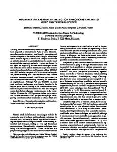
Although not usually seen in this way, stand density management diagrams (SDMDs, Drew and Flewelling, 1979) are an attempt at modelling stand development in a two-dimensional state space. Farnden (1996) produced SDMDs for several species based on TIPSY. First, Eichhorn’s hypothesis is used to deal with site quality. TIPSY utilizes a principle advanced by Eichhorn, found approximately valid in other studies (Eichhorn, 1904; Assmann, 1970), which in its extended form says that the relationship between any state variable and top height is independent of site quality. That is, curves of stand volume or tree diameter over top height are the same for all sites, only the speed of movement along the curve changes. Therefore, growth relative to height increment is modelled in a site-independent manner, and the relationship between height and age is obtained separately through a conventional site index model. Eichhorn’s hypothesis is not used in TASS, but graphing predictions showed that it was generally a good approximation (Mitchell and Cameron, 1985). As usual, the state variables in Farnden’s SDMDs are the number of trees per hectare, N , and the mean tree volume, v, plotted on logarithmic axes (some authors use mean dbh instead of v; for reviews see Ernst and Knapp (1985), Jack and Long (1996), Newton (1997)). The simulations from the TIPSY planted Douglas-fir database are shown in Figure 1. Successive points for each stand are at 3-metre top height1 steps, and are joined by lines. The first point for unthinned stands is at 3 m top height. Thinned stand trajectories start at the time of thinning: 6 m top height for “pre-commercial” and 21–33 m for “commercial” thinnings. SDMDs assume that the changes in N and v per unit of height depend only on their current values, generating a unique trajectory through each point in the graph. In symbols, dN dH
= f1 (N, v)
(1a)
1 The B. C. Forest Productivity Council standards reserve the term “top height” for a specific sampling protocol. The recommended alternative “site height” has been adopted for TADAM’s computer programs and documentation, but I use here the more widely accepted terminology.
3
FBMIS Volume 1, 2003, 1–15
ISSN 1740-5955
c 2003 The FBMIS Group Copyright °
http://www.FBMIS.info/A/3 1 GarciaO 1
10
unthinned precommercial commercial
Mean tree volume (m3)
1
0.1
0.01
0.001
0.0001 100
1000 Trees per hectare
10000
Figure 1: TASS simulations in the TIPSY database , on a stand density management diagram framework (see text). Tic marks on the trajectories indicate TIPSY’s 3-metre intervals.
dv dH
= f2 (N, v) .
(1b)
Similar pairs of differential equations have been used by Hara (1984), Tait (1988), and Turnblom and Burk (2000). On a SDMD trajectories are indicated graphically, and visually interpolated, guided by a hypothesized limiting self-thinning line on the log-log scale. In order to keep track of height (and time), curves called height isolines are drawn across equal-height points on the diagram. It is assumed that the changes of state caused by thinning follow the isolines. It can be seen from Figure 1, however, that thinned and unthinned equalheight points are not aligned. Actually, the increase in mean volume from the removal of a given number of stems depends of the selectivity of the thinning, and there is no apparent reason why the before and after thinning points should fall on a same isoline. It would be possible to correct this logical flaw of SDMDs through a somewhat more complex growth projection procedure, adding thinning curves and interpreting distances between isolines in relative terms. Weller (1987) points out that the usual plotting of self-thinning data can be misleading. The logarithms obscure the trends by clustering data at one end of the volume scale. In addition, the total volume per hectare V may be more meaningful than v = V /N , and having N on both axes makes relationships appear stronger than they really are. In Figure √ 2, V is used instead of log v in the vertical axis. I have used the average spacing S = 100/ N to achieve a more even horizontal data distribution. Clearly, any one-to-one transformation of the state vector is an equally valid stand descriptor, and equations analogous to (1) would apply. It is now possible to see that there is no obvious unique self-thinning limit. Note also the irregularities due to the stochastic nature of TASS. More importantly, the crossing of trajectories indicates that these two variables do not constitute a satisfactory state vector — different rates of change are observed for the same state. We conclude that the dynamics of thinned stands in TASS cannot be well approximated in two dimensions, at least not with the variables used in the stand density management diagrams. In fact, Farnden (1996) warns that his projections for commercial thinning may be unreliable. This agrees with observations from thinned radiata pine permanent sample plots in New Zealand (Garc´ıa, 1990, 1993). It may be significant that most of the published work on SDMDs and self-thinning has used data from unmanaged stands. 4
FBMIS Volume 1, 2003, 1–15
ISSN 1740-5955
c 2003 The FBMIS Group Copyright °
http://www.FBMIS.info/A/3 1 GarciaO 1
2000
unthinned precommercial commercial
1800 1600 Volume (m3/ha)
1400 1200 1000 800 600 400 200 0 1
2
3 4 5 Average spacing (m)
6
7
Figure 2: The TIPSY database, alternative axis transformation. Lines illustrate simulated development of individual stands. In what follows, I therefore examine the possibility of approximating TASS by including a third state variable. A natural variable to add is the top height, H. In three dimensions a graphical prediction approach becomes impractical, and equations are necessary to describe the rates of change of state.
5
RATE EQUATIONS
Instead of V it seems preferable to use as state variable the closely related “bulk” W ≡ BH, where B is basal area per hectare. Basal area is more directly measured, and is not affected by artificial differences in volume tables and utilization standards. Analogous to (1), we search then for an appropriate pair of rate equations, or local transition functions: dN dH dW dH
= f1 (N, W, H)
(2a)
= f2 (N, W, H) .
(2b)
The third rate equation, for H, is trivial (dH/dH = 1). 5.1 Mortality. In TASS, tree growth and competition are driven by crown dimensions, height, and growing space. The amount of dead xylem accumulated on the stem is considered biologically irrelevant. As seems logical, and unlike in most other individual-tree models, variables such as tree diameter, basal area, or stem volume have no place as predictors of gross increment or tree mortality in TASS. Hence, we can expect the mortality rate (2a) to be mostly a function of N and H. TIPSY yield table data was plotted in a number of ways to explore the mortality relationships, including the use of 3-D dynamic graphics. Derivatives were approximated by central finite differences. After considering various alternatives, it was found that the limiting behaviour of the relative mortality rate −(dN/dH)/N = −d ln N/dH could be represented by an equation of
5
FBMIS Volume 1, 2003, 1–15
ISSN 1740-5955
c 2003 The FBMIS Group Copyright °
http://www.FBMIS.info/A/3 1 GarciaO 1
the form
d ln N = −a exp[b(ln N − ln N∞ ) − ab(H∞ − H)] , (3) dH where N∞ and H∞ are asymptotic values for N and H, respectively. Young, open-growing stands would have negligible mortality, as expected from the description of TASS in Mitchell (1975). This equation can be easily integrated analytically. In the TIPSY tables, however, there is a substantial amount of mortality in the initial years. Graphs revealed that the current version of TASS adds a relative mortality rate decreasing linearly with top height, from an initial value of about 1.7% per metre, down to zero at 15 or 16 metres top height. Discontinuities can cause trouble in optimization applications. I decided to sacrifice some goodness of fit by adding a more aesthetically pleasing decreasing exponential instead of the linear segment. Unfortunately, the modified equation requires numerical integration, somewhat complicating the model estimation and usage. This relationship would probably be sufficient if we were modelling field observations. But the main objective here was to see how closely an aggregated stand-level model could approximate a complex tree-level model. With numerical integration already needed, and over-parameterization not an issue, it was decided to try optimizing the fit through a “fine-tuning” polynomial factor. Including in (3) the added exponential term and a second-degree polynomial in ln N , BH and H, the mortality model can be written as d ln N = −(a1 e−a2 H + a3 N a4 ea5 H )P , dH
(4)
with P
=
1 + b1 ln N + b2 BH + b3 H +b4 (ln N )2 + b5 (BH)2 + b6 H 2 +b7 BH ln N + b8 H ln N + b9 BH 2 .
The ai and bi are parameters to be estimated. 5.2 Volume, basal area. Searching for an appropriate functional form for (2b) was done with the total volume per hectare V , taking advantage of the presence of gross volumes in the yield tables. Net volume increment, relative to height increment, was modelled as the difference between gross volume increment and mortality. Similar approaches have been used by Beekhuis (1966), and Garc´ıa and Ruiz (2003). As already mentioned, from the workings of TASS we can expect gross increment to be a function of N and H, but not of V or B. After some trial-and-error, the following form appeared satisfactory: 2 (a6 + a7 H)(1 − e−a8 N H ) . (5) The mortality in terms of volume per hectare may be written as the product of the mortality in number of trees, the average tree volume, and some factor less than one that represents the fact that dead trees tend to be smaller than average: −k
V dN d ln N = −kV . N dH dH
The proportionality factor k may vary with the state of the stand. Values of k calculated from consecutive points in the yield tables were related to the state variables graphically and through logarithmic regression. Good results were obtained with k proportional to a power of H. Subtracting the mortality from (5), substituting the surrogate W = BH for V , and including a fine-tuning polynomial, we have the model 2 d ln N dBH = [(a6 + a7 H)(1 − e−a8 N H ) + a9 BH a10 ]Q , dH dH
with Q =
1 + c1 ln N + c2 BH + c3 H +c4 (ln N )2 + c5 (BH)2 + c6 H 2 +c7 BH ln N + c8 H ln N + c9 BH 2 . 6
(6)
FBMIS Volume 1, 2003, 1–15
ISSN 1740-5955
c 2003 The FBMIS Group Copyright °
http://www.FBMIS.info/A/3 1 GarciaO 1
5.3 Parameter estimation. To complete the growth relationships, values for the parameters ai , bi and ci are needed. These were estimated from the values of H, B and N contained in the yield table database for planted Coastal Douglas-fir of TIPSY version 3.0. The yield tables were generated with TASS version 2.05.24b, in October 1997 (K. Polsson, pers. comm.). The tables have values at 3 m top-height intervals, up to a maximum of 60 m (175 years of age for Mitchell’s (1975) reference site index 35, or 363 years for a medium-quality site index of 30). TASS runs were based on a set of tree spacings of 1.5, 2.0, . . . , 5.5 m. Simulations started with these square planting spacings, so that there are 9 unthinned tables. Pre-commercial thinnings were simulated at top height 6 m, up to all the feasible average spacings in the set, making 20 combinations. Similarly, commercial thinnings were simulated at heights of 21, 27 and 33 m, with and without a previous pre-commercial thinning, producing another 147 alternatives. In all, there are 176 treatments, with a total of 2324 unique “observations”(Figures 1, 2). The situation here is different from estimating parameters with field measurements, where the error structure in the observations should be taken into account (e. g., Garc´ıa, 1994). I tried, instead, to reproduce the TASS simulations as closely as possible, by minimizing the discrepancies over whole trajectories. The system of differential equations formed by (4) and (6) was integrated with a 4th-order Runge-Kutta method (Press et al., 1993), using 3-metre steps (smaller step lengths showed no appreciable differences). To avoid duplication, thinned projections were started from the values after the last (or only) thinning. For unthinned stands, I added an initial point at 1.3 m top height (breast height) with zero basal area, and a first integration step of 3 − 1.3 = 1.7 m. The number of trees per hectare at 1.3 m was calculated multiplying the number planted by 0.978, the average survival rate in the simulations. Various criteria may be used to assess “closeness”. The most common one evaluates error by the sum of squares of the deviations. Another, the minimax criterion, calculates the maximum absolute deviation over all the data. Intermediate error measures are possible, based on the sum of n-powers of the absolute deviations; n = 2 gives the usual least-squares, and minimax is approximated as n → ∞. These were implemented in a program written in C. For each yield table in the database, the program integrates (4) and (6) at 3 m intervals up to a height of 60 m, with either the after-thinning or the breast-height point as initial condition. A minimum for the selected error criterion over the set of parameters was sought with a general-purpose numerical unconstrained optimization algorithm. I used the optimization routine OPVM (N. O. C., 1976), converted from Fortran to C with f2c (Feldman et al., 1990). OPVM had been successfully applied to a number of complex estimation problems in the past (Garc´ıa, 1984). Good initial parameter estimates are important for successful convergence of the optimization. Difficulties often arise from overflows and out-of-range exceptions in exponentials, powers and logarithms. To mitigate these problems variables were scaled to make them closer to unity, dividing B by 100, N by 1000, and H by 10. It was useful to proceed by introducing a few free parameters at a time, building up to more general models through a sequence of runs. Fitting strategies were roughly as follows. I started with equation (4) without the polynomial, which does not involve B. Parameters were estimated based on the deviations of ln N , that are approximately equivalent to relative errors in number of trees per hectare. Given the mortality equation, (6) without the polynomial Q was fitted, minimizing deviations in B. Using this for basal area predictions, (4) was re-estimated including the polynomial, introducing additional parameters in stages, first the linear terms and then the rest. Fixing the mortality parameters, the same was then done for the full equation (6). The two fitting stages were repeated, to account for interactions; changes beyond a second iteration were negligible. Perturbation of initial parameter values guarded against possible local optima. In practice, programming revisions and adjustments provided additional runs with various starting points, which confirmed the consistency of the solutions. 5.4 Results. As might have been expected in retrospect, minimax runs stopped short of producing reasonable estimates. Data irregularities due to stochastic variation, and in part to rounding in the yield tables, cause numerous local optima in the minimax function that interrupt global convergence. Predictions from the n-th power criteria with n other than 2 conferred no visible advantage. Therefore, the least-squares estimates were used. Without the polynomial factor, the root-mean-square error (RMSE) for ln N was 0.0335, equivalent to approximately 3.4% for N . The fine-tuning polynomial had a relatively small effect, reducing this to 0.0272 (2.7%). For B, the RMSE without the polynomials was 2.34 m2 /ha,
7
FBMIS Volume 1, 2003, 1–15
ISSN 1740-5955
c 2003 The FBMIS Group Copyright °
http://www.FBMIS.info/A/3 1 GarciaO 1
Table 1: Parameter estimates for (4), (6) i ai bi ci 1 0.226788 0.566735 -0.223694 2 1.99265 -0.577931 0.231860 3 2.37237 · 10−5 0.532844 -0.355166 4 4.26397 -0.0425355 0.0594313 5 2.99041 0.121589 -0.0191612 6 -0.14782 -0.166314 0.0486283 7 0.838876 0.766793 -0.0669217 8 0.896480 -0.874513 0.126619 9 0.193436 0.0251072 -0.0215096 10 1.68922 — — decreasing to 1.10 m2 /ha for the full model. As previously mentioned, it seems worthwhile here to use the full parameter set. Parameter values are given in Table 1, for variables scaled as indicated before: N in trees per hectare, B in m2 /ha, and H in metres, divided by 1000, 100, and 10, respectively. The fit of the mortality model is illustrated in Figure 3, for the unthinned stands. It is apparent that discrepancies are largely due to stochastic variation, and that a much better agreement cannot be expected from a smooth deterministic model.
Trees per hectare
TASS/TIPSY TADAM
1000
0
10
20
30 Top height (m)
40
50
60
Figure 3: Mortality trends from the TASS/TIPSY unthinned yield tables (solid curves), and corresponding TADAM projections from the same initial state (dashed). Logarithmic N -scale. A similar graph for basal area is shown in Figure 4. The fit can be better appreciated in Figure 5, where the basal area residuals, that is, the difference between the TASS/TIPSY values and the TADAM projections, are displayed. There are no obvious systematic departures, with differences being mostly within ±2 m2 /ha.
8
FBMIS Volume 1, 2003, 1–15
ISSN 1740-5955
c 2003 The FBMIS Group Copyright °
http://www.FBMIS.info/A/3 1 GarciaO 1
120
TASS/TIPSY TADAM
Basal area (m2/ha)
100
80
60
40
20
0 0
10
20
30
40
50
60
Top height (m) Figure 4: Basal area trends from the TASS/TIPSY unthinned yield tables (solid curves), and corresponding TADAM projections from the same initial state (dashed).
6
unthinned precommercial commercial
5 4 Basal area (m2/ha)
3 2 1 0 -1 -2 -3 -4 -5 0
10
20
30 Top height (m)
40
Figure 5: Basal area residuals, full data set.
9
50
60
FBMIS Volume 1, 2003, 1–15
ISSN 1740-5955
c 2003 The FBMIS Group Copyright °
http://www.FBMIS.info/A/3 1 GarciaO 1
6
AUXILIARY RELATIONSHIPS AND OUTPUT FUNCTIONS
Besides the rate equations, which predict the change in state variables during free growth, some additional relationships are needed to apply the model in practice. First, height must be related to age and site quality. Sometimes, missing information about thinning transitions needs to be estimated. Finally, output variables of interest, such as various measures of volume, have to be estimated from current state values. 6.1 Height-age, site. The same model as in TIPSY was used for relating top height, age and site quality. It is a metric version of the site index model of Bruce (1981): H b2 b3
= S exp{b2 [(t + t0 + 1)b3 − (63.25 − S/6.096)b3 ]} b3
(7) b3
= ln(1.372/S)/[(13.25 − S/6.096) − (63.25 − S/6.096) ] = −0.477762 − 0.894427(S/30.48) + 0.793548(S/30.48)2 −0.171666(S/30.48)3 ,
where S is site index, t is age from planting, and t0 is a “time gain” parameter used for shifting the height-age curves horizontally. Site index is based on a breast-height age of 50 years with a breast-height of 1.372 m, not the standard 1.3. The time gain is normally zero, but can be used to adjust for atypical establishment conditions (Garc´ıa, 1996); in TIPSY, the negative of t0 appears as “regeneration delay”. Given S and t0 , (7) can be used to estimate top height at any age. The equation is easily inverted to estimate age for a given height, or time gain given height, age, and site. The model implementations also provide a numerical procedure to estimate site index knowing height and age. We note that TADAM is actually age-independent, in the sense that if there is a separate estimate of site index, perhaps obtained through Biogeoclimatic Ecosystem Classification methods (Green et al., 1989; B. C. Ministry of Forests, 1997), age is not needed for projecting future growth. This could be useful in some inventory situations where reliable estimates of age are not available. 6.2 Thinning. In terms of the model, a thinning is simply an instantaneous change in basal area and trees per hectare. For thinnings from below, changes in top height can be ignored. Thinnings are often specified by number of trees left or removed, and it can be useful to have a relationship for the corresponding change in basal area. Conversely, sometimes the change in number of trees needs to be estimated from thinned or residual basal area. Garc´ıa (1984) modelled the process of thinning with a differential equation relating the incremental relative changes in basal area and numbers of trees to the current state: d ln B = aB b N c H d . d ln N Integrating, if b, c 6= 0,
ab d c H (N0 − N c )]/b , (8) c where B0 and N0 are values before thinning, and B and N are after thinning. Non-linear regression with the TIPSY database thinnings (n = 541) gave the parameter estimates a = 181.30, b = 0.57086, c = −0.55678, d = −1.2987, all significant (p ¿ 0.01). The standard error of estimate was 0.04943, approximately 5% of the basal area. I used the inverse of (8) to estimate N from B. Note that this equation reflects the selectivity of the particular simulated thinning algorithm used, described in TIPSY’s Help. ln B = − ln[B0−b +
Volume. Volume can be estimated from the state variables with stand volume equations. Total standing volume from the yield tables was fitted by stepwise linear regression, with various dependent variable transformations. Best results were obtained with V /B, where V is the volume in cubic metres per hectare: √ (9) V /B = 0.15471 + 0.49184H − 0.067306B − 1.5458H/ N + 0.00018096N H/B . 6.3
Standard error was 0.3166 m, with 2487 points (excluding two that had zero volume). 10
FBMIS Volume 1, 2003, 1–15
ISSN 1740-5955
c 2003 The FBMIS Group Copyright °
http://www.FBMIS.info/A/3 1 GarciaO 1
TIPSY provides merchantable volumes, excluding a 10 cm top and 30 cm stump, for trees above dbh limits of 12.5, 17.5, 22.5, 27.5, 32.5 cm. I modelled the merchantable to total volume ratio M/V as a continuous function of the limit dbh d. Graphs showed high noise levels, suggesting that the diameter distribution is very sensitive to the stochastic variation in TASS. Satisfactory estimates were obtained with the non-linear regression M/V = 0.93296N −0.021463 D0.040375 exp(−0.89470H −2.4420 D−4.6721 d6.7564 ) ,
(10)
where D is the (quadratic) mean dbh, in centimetres. Residual standard error for the ratio was 0.01724, on 11593 degrees of freedom (a few points with zero total volume or small dbh were omitted). Under some circumstances (10) can predict a volume increase from thinnings near the merchantability threshold, overestimating the effect of the rise in mean dbh. This is unlikely to be important in practice, but it would be nice to develop a better-behaved equation form. On occasion, more detailed size distribution information may be desirable. This is generated by individual-tree models in a fairly direct way. In whole-stand models, distribution parameters can be estimated from current state values. For instance, Garc´ıa (1984) regressed the dbh coefficient of variation on the state variables, fitting a Weibull distribution by the method of moments. Because the required data was not readily available this was not attempted here. Regardless of the approach, however, the limitations of distribution simulations and modelling should be kept in mind. Huge sample sizes would be needed for precise distribution shape estimation, and shape and variance change with plot size due to spatial correlation (Garc´ıa, 1992, 1994, and references therein). As with other individual-tree models, TASS currently ignores any positive microsite-induced spatial correlation, although in reality this positive autocorrelation often dominates the negative one arising from competition (op. cit.).
7
IMPLEMENTATION
Two computer implementations of the model have been completed to date. The first is a stand-alone interactive simulator running on Palm-compatible hand-held devices (Rey et al., 2000). It was written in C, using the CodeWarrior development system (Metrowerks, 2000; Foster, 2000), and occupies 44 Kb of memory. The Palm simulator can be initiated from any existing stand conditions, or with a newly planted stand. In this last instance, calculations start at top height 1.3 m, with zero basal area and a number of trees per hectare of 0.978 times the nominal initial density. Simulation can proceed forward or backward in time, displaying results at any specified age or top height interval. Internally, the system (4), (6) is integrated with a 4th-order Runge-Kutta algorithm, if necessary subdividing the integration interval into equal-size steps of no more than 4 m. Thinnings may be simulated at any time, specifying intensity in trees per hectare, basal area, or both. Output can be saved for graphing or further processing in spreadsheets or other software. It is also possible to run the simulator on a Palm emulator in Windows, Mac, or Unix/Linux computers. The second implementation consists of the same basic C routines from the simulator, with some cover functions to make them easy to call from other computer software. For Windows, this has been packaged in a dynamic linked library (DLL). Gyula Gulyas, from Olympic Resource Management, has used the DLL in a Microsoft Excel add-in that accesses the code as ordinary spreadsheet functions. Growth projection takes as input a current state, (N, B, H), and returns the state for any other given top height. Height-age, age-height, and site index estimation functions complete the tools required for simulating stand dynamics. In addition, thinning estimates based on (8) and its inverse, and volume outputs (9) and (10), are provided. The software is freely available from http://www.unbc.ca/forestry/forestgrowth/tadam.
8
DISCUSSION AND CONCLUSIONS
Spatial individual-tree growth models are important research tools, facilitating the synthesis of existing biological knowledge, testing of hypotheses, and identification of gaps in information. They could also play a useful role in early forestry development stages, where little or no observational data are available. At least for single species even-aged stands, however, aggregated whole-stand models may be preferable for forest management planning applications.
11
FBMIS Volume 1, 2003, 1–15
ISSN 1740-5955
c 2003 The FBMIS Group Copyright °
http://www.FBMIS.info/A/3 1 GarciaO 1
Doing away with largely redundant details, they can make better use of available inventory information and, given adequate permanent sample plot data, potentially produce more precise predictions2 . Parsimonious, well-behaved models are particularly desirable for embedding into integrated decision-support systems. The popularity of stand density management diagrams suggests a demand for simpler, easy-to-use tools. The success of SDMDs in describing the development of unthinned stands established at different initial densities has been explained by Garc´ıa (1993) as a mathematical consequence of system dynamics. Briefly, at any time stands of all possible densities lie on a curve in the state space. For instance, in TADAM’s 3-dimensional state space a convenient starting curve would be the straight line defined by H = 1.3, B = 0. As stands develop, the moving curve generates a surface (Figures 3–4). Therefore, a two-dimensional projection along a direction where the surface does not exhibit “folds” produces a valid pair of state variables for unthinned stands. The SDMD variants described in the literature can be seen as projections onto various two-dimensional state spaces, possibly combined with single-variable transformations (e. g., logarithms). A thinning, however, in general causes a stand to leave the surface, and two-dimensional projections of rate vectors at different levels do not necessarily coincide. It might be possible to find specific projections for which differences are small, a topic for further research. TADAM has shown that with three state variables TASS projections seem to be reproduced sufficiently accurately for practical use. Figure 5 suggests a slight growth over-prediction immediately following commercial thinning, presumably due to a temporary loss of full site occupancy. An additional state variable can improve predictions after heavy thinning and pruning, and help in modelling effects of defoliation from pests, etc., at the cost of added complexity in model usage (Garc´ıa, 1990, 1994; Garc´ıa and Ruiz, 2003). Most of the discrepancies seem due to the stochastic variation in TASS. Although at first sight it might appear paradoxical, TADAM predictions could be closer to those of TASS than the TASS-generated yield tables on which they were based. The TIPSY database yield tables are individual stochastic realizations, which may differ considerably from what would be the theoretically expected or most likely prediction from TASS. TADAM smoothes-out trends using information from the whole database. In fact, this situation seems common in forest modelling. One of the advantages often claimed for stochastic growth models is the provision of realistic information on the variability to be expected. In practice, however, decisions appear to be generally made based on single simulation instances. At least some averaging over different random number sequences would seem desirable for management applications. Multiple runs would also allow a more thorough evaluation of TADAM’s goodness of fit, even though single realizations are somewhat more efficient in covering a wider range of stand conditions for a given sample size. Unfortunately, TASS is not easily accessible for extensive experimentation, being only available through Ministry of Forests personnel on their own computer. The impact of stochasticity may be illustrated by Figure 6, where periodic gross volume increments predicted in the TIPSY yield tables are plotted over height. The consistent fluctuation pattern across simulations appears due to the use of a common pseudo-random sequence (data perturbation tests ruled out rounding as a possible cause). This persistence of the random seed effect might be somewhat surprising, considering the differences in initial conditions. Using a fixed random seed may improve treatment comparisons, but it also introduces artificial features that are not paralleled by the aggregated model. The current implementations of TADAM have few of TIPSY’s numerous output variables and options. In a sense, both approximate and interpolate output from TASS. Instead of interpolating whole trajectories, however, TADAM interpolates directional vectors (rates). This allows greater flexibility, making it possible to simulate any combination of thinning timings and intensities. As already mentioned, however, the main significance of TADAM may lie in demonstrating the feasibility of reducing dimensionality with little loss of information. A logical next step would produce whole-stand models based directly on field data. 2 Many inventories provide tree lists, which are taken as representative of a dbh distribution in distanceindependent individual-tree models. Problems with high sampling error and with spatial correlation effects have already been mentioned. In addition, it is a “local distribution” for neighbouring competing trees which is relevant to tree growth, and correlations between dbh and growing space are weakened under stand density management. At some point using unreliable data becomes counterproductive, compared to discarding it in favour of prior knowledge. I believe that for distribution shape the cutoff is likely to lie well beyond normal sample sizes, although more research on this is needed.
12
FBMIS Volume 1, 2003, 1–15
ISSN 1740-5955
c 2003 The FBMIS Group Copyright °
http://www.FBMIS.info/A/3 1 GarciaO 1
3m gross volume increment (m3/ha)
200
unthinned precommercial commercial
180 160 140 120 100 80 60 40 20 0 0
10
20
30 Top height (m)
40
50
60
Figure 6: Gross volume increments for each 3-metre top height interval in the TIPSY database. Consecutive values from each TASS simulation are joined by straight lines, plotted over the interval initial height.
REFERENCES Assmann, E. (1970) The Principles of Forest Yield Study. Pergamon Press. B. C. Ministry of Forests (1997) Site index estimates by site series for coniferous tree species in British Columbia. British Columbia Ministry of Forests, Forest Practices Branch. Victoria, B.C. Beekhuis, J. (1966) Prediction of yield and increment in Pinus radiata stands in New Zealand. Technical Paper 49, Forest Research Institute, NZ Forest Service. Bruce, D. (1981) Consistent height-growth and growth-rate estimates for remeasured plots. Forest Science 27, 711–725. Di Lucca, C. M. (1998) TASS/SYLVER/TIPSY: systems for predicting the impact of silvicultural practices on yield, lumber value, economic return and other benefits. In: Bamsey, C. R. (ed.) Stand Density Management Conference: Using the Planning Tools. November 23–24, 1987, Edmonton, Alberta. Alberta Environmental Protection, pp. 7–16. Drew, T. J. and Flewelling, J. W. (1979) Stand density management: an alternative approach and its application to Douglas-fir plantations. Forest Science 25, 518–532. Eichhorn, F. (1904) Beziehungen zwischen Bestandsh¨ohe und Bbestandsmasse. Allgemeine Forst- und Jagdzeitung 80, 45–49. Ernst, R. L. and Knapp, W. H. (1985) Forest stand density and stocking: concepts, terms, and the use of stocking guides. General Technical Report WO-44, USDA Forest Service. Farnden, C. (1996) Stand density management diagrams for lodgepole pine, white spruce and interior Douglas-fir. Information Report BC–X–360, Canadian Forest Service, Pacific Forestry Centre, Victoria, British Columbia. Feldman, S. I., Gay, D. M., Maimone, M. W. and Schryer, N. L. (1990) A Fortran-to-C converter. Computing Science Technical Report 149, AT&T Bell Laboratories, Murray Hill, NJ 07974. Foster, L. R. (2000) Palm OS Programming Bible. IDG Books Worldwide Inc., Foster City, CA. Garc´ıa, O. (1984) New class of growth models for even-aged stands: Pinus radiata in Golden Downs Forest. New Zealand Journal of Forestry Science 14, 65–88. Garc´ıa, O. (1990) Growth of thinned and pruned stands. In: James, R. N. and Tarlton, G. L. 13
FBMIS Volume 1, 2003, 1–15
ISSN 1740-5955
c 2003 The FBMIS Group Copyright °
http://www.FBMIS.info/A/3 1 GarciaO 1
(eds.) New Approaches to Spacing and Thinning in Plantation Forestry: Proceedings of a IUFRO Symposium, Rotorua, New Zealand, 10–14 April 1989. Ministry of Forestry, FRI Bulletin No. 151, pp. 84–97. Garc´ıa, O. (1992) What is a diameter distribution? In: Minowa, M. and Tsuyuki, S. (eds.) Proceedings of the Symposium on Integrated Forest Management Information Systems — An International Symposium — October 13–18, 1991, Tsukuba, Japan. Japan Society of Forest Planning Press, pp. 11–29. Garc´ıa, O. (1993) Stand growth models: Theory and practice. In: Advancement in Forest Inventory and Forest Management Sciences — Proceedings of the IUFRO Seoul Conference. Forestry Research Institute of the Republic of Korea, pp. 22–45. Garc´ıa, O. (1994) The state-space approach in growth modelling. Canadian Journal of Forest Research 24, 1894–1903. Garc´ıa, O. (1996) Easy evaluation of establishment treatments. In: Klemperer, W. D. (ed.) Proceedings of the S4.04 Meetings on Forest Management Planning and Managerial Economics, IUFRO 20th World Congress, Tampere, Finland, August 6–12, 1995. Virginia Polytechnic Institute and State University, College of Forestry and Wildlife Resources, Publication No. FWS 1–96, pp. 89–94. Garc´ıa, O. (2001) On bridging the gap between tree-level and stand-level models. In: Rennolls, K. (ed.) Proceedings of IUFRO 4.11 Conference “Forest Biometry, Modelling and Information Science”, University of Greenwich, June 25-29, 2001. http://cms1.gre.ac.uk/conferences/iufro/proceedings. Garc´ıa, O. and Ruiz, F. (2003) A growth model for eucalypt in Galicia, Spain. Forest Ecology and Management 173, 49–62. Goudie, J. W. (1998) Model validation: A search for the magic grove or the magic model. In: Bamsey, C. (ed.) Stand density management: Planning and implementation. Edmonton, Alberta, pp. 45–58. Green, R. N., Marshall, P. L. and Klinka, K. (1989) Estimating site index of Douglas-fir (Pseudotsuga menziesii [Mirb] Franco) from ecological variables in southwestern British Columbia. Forest Science 35, 50–63. Hara, T. (1984) Modelling the time course of self-thinning in crowded plant populations. Annals of Botany 53, 181–188. Jack, S. B. and Long, J. N. (1996) Linkages between silviculture and ecology: an analysis of density management diagrams. Forest Ecology and Management 86, 205–220. Larson, P. R. (1963) Stem form development of forest trees. Forest Science Monograph 5, Society of American Foresters. Metrowerks (2000) CodeWarrior — Targeting the Palm OS platform. Metrowerks Corporation, Austin, TX. Mitchell, K. J. (1969) Simulation of the growth of even-aged stands of white spruce. School of Forestry Bulletin No. 75, Yale University, New Haven, CT. Mitchell, K. J. (1975) Dynamics and simulated yield of Douglas-fir. Forest Science Monograph 17, Society of American Foresters. Mitchell, K. J. and Cameron, I. R. (1985) Managed stand yield tables for coastal Douglas-fir: Initial density and precommercial thinning. Land Management Report 31, B. C. Ministry of Forests, Research Branch, Victoria, British Columbia. Mitchell, K. J., Grout, S. E., Macdonald, R. N. and Watmough, C. A. (1992) User’s guide for TIPSY: A Table Interpolation Program for Stand Yields. B. C. Ministry of Forests, Research Branch, Victoria, B. C. N. O. C. (1976) OPTIMA — Routines for optimisation problems. Numerical Optimisation Centre, The Hatfield Polytechnic. Newton, P. F. (1997) Stand density management diagrams: Review of their development and utility in stand-level management planning. Forest Ecology and Management 98, 251–265. Press, W. H., Flannery, B. P., Teukolski, S. A. and Vetterling, W. T. (1993) Numerical Recipes in C: The Art of Scientific Computing. Cambridge University Press, 2nd edn. Rey, C., Freeman, E. and Ostrem, J. (2000) Palm OS SDK reference. Document Number 3003003, Palm, Inc., Santa Clara, CA. Shinozaki, K. K., Yoda, K., Hozumi, K. and Kira, T. (1964) A quantitative analysis of plant form — the pipe model theory. I. Basic analyses. Japanese Journal of Ecology 14, 97–105. Tait, D. E. (1988) The dynamics of stand development: a general stand model applied to Douglas-
14
FBMIS Volume 1, 2003, 1–15
ISSN 1740-5955
c 2003 The FBMIS Group Copyright °
http://www.FBMIS.info/A/3 1 GarciaO 1
fir. Canadian Journal of Forest Research 18, 696–702. Turnblom, E. C. and Burk, T. E. (2000) Modeling self-thinning of unthinned Lake States red pine stands using nonlinear simultaneous differential equations. Canadian Journal of Forest Research 30, 1410–1418. Vanclay, J. K. (1994) Modelling Forest Growth and Yield: Applications to Mixed Tropical Forests. CABI International. Weller, D. E. (1987) A reevaluation of the -3/2 power rule of plant self-thinning. Ecological Monographs 57, 23–43.
15