Dirac Fields in Loop Quantum Gravity and Big Bang Nucleosynthesis

ESI

The Erwin Schr¨ odinger International Institute for Mathematical Physics

Boltzmanngasse 9 A-1090 Wien, Austria

Dirac Fields in Loop Quantum Gravity and Big Bang Nucleosynthesis

Martin Bojowald Rupam Das Robert J. Scherrer

Vienna, Preprint ESI 1972 (2007)

Supported by the Austrian Federal Ministry of Education, Science and Culture Available via http://www.esi.ac.at

November 2, 2007

Dirac Fields in Loop Quantum Gravity and Big Bang Nucleosynthesis Martin Bojowald Institute for Gravitation and the Cosmos, The Pennsylvania State University, 104 Davey Lab, University park, PA

16802

Rupam Das Department of Physics and Astronomy, Vanderbilt University, Nashville, TN 37235 and Institute for Gravitation and the Cosmos, The Pennsylvania State University, 104 Davey Lab, University park, PA

16802

Robert J. Scherrer Department of Physics and Astronomy, Vanderbilt University, Nashville, TN

37235

Big Bang nucleosynthesis requires a fine balance between equations of state for photons and relativistic fermions. Several corrections to equation of state parameters arise from classical and quantum physics, which are derived here from a canonical perspective. In particular, loop quantum gravity allows one to compute quantum gravity corrections for Maxwell and Dirac fields. Although the classical actions are very different, quantum corrections to the equation of state are remarkably similar. To lowest order, these corrections take the form of an overall expansion-dependent multiplicative factor in the total density. We use these results, along with the predictions of Big Bang nucleosynthesis, to place bounds on these corrections. PACS numbers: 04.20.Fy, 04.60.Pp,98.80.Ft

I.

INTRODUCTION

Much of cosmology is well-described by spatially isotropic Friedmann–Robertson–Walker models with line elements   dr 2 2 2 2 2 2 2 2 + r (dϑ + sin ϑdϕ ) (1) ds = −dτ + a(τ ) 1 − kr 2 where k = 0 or ±1, sourced by perfect fluids with equations of state P = wρ. Such an equation of state relates the matter pressure P to its energy density ρ and captures the thermodynamical properties in a form relevant for isotropic space-times in general relativity. Often, one can assume the equation of state parameter w to be constant during successive phases of the universe evolution, with sharp jumps between different phases such as w = −1 during inflation, followed by w = 31 during radiation domination and w = 1 during matter domination. Observationally relevant details can depend on the precise values of w at a given stage, in particular if one uses an effective value describing a mixture of different matter components. For instance, during big bang nucleosynthesis one is in a radiation dominated phase mainly described by photons and relativistic fermions. Photons, according to Maxwell theory, have an exact equation of state parameter w = 13 as a consequence of conformal invariance of the equations of motion (such that the stress-energy tensor is trace-free). For fermions the general equation of state is more complicated and non-linear, but can in relativistic regimes be approximately given by the same value w = 31 as for photons. In contrast to the case of Maxwell theory, however, there is no strict symmetry such as conformal invariance which would prevent w to take a different value. It is one of the main objectives of the present paper to discuss possible corrections to this value. For big bang nucleosynthesis, it turns out, the balance between fermions and photons is quite sensitive. In fact, different values for the equation of state parameters might even be preferred phenomenologically [1]. One possible reason for different equations of state might be different coupling constants of bosons and fermions to gravity, for which currently no underlying mechanism is known. In this paper we will explore the possibility whether classical as well as quantum corrections to the equations of state can produce sufficiently different values for the equation of state parameters. In fact, since the fields are governed by different actions, one generally expects different, though small, correction terms which can be of significance in a delicate balance. An approach where quantum gravitational corrections can be computed is loop quantum cosmology [2], which specializes loop quantum gravity [3–5] to cosmological regimes. In such a canonical quantization of gravity, equations of state must be computed from matter Hamiltonians rather than covariant stress-energy tensors. Quantum corrections to the underlying Hamiltonian then imply corrections in the equation of state. This program was carried out for the Maxwell Hamiltonian in [6], and is done here for Dirac fermions. There are several differences between the treatment of fermions and other fields, which from the gravitational point of view are mainly related to the fact that fermions, in a first order formulation, also couple to torsion and not just the curvature of space-time. After describing the

classical derivation of equations of state as well as steps of a loop quantization and its correction terms, we use big bang nucleosynthesis constraints to see how sensitively we can bound quantum gravity parameters. We have aimed to make the paper nearly self-contained and included some of the technical details. Secs. II on the canonical formulation of fermions, III on quantum corrections from loop quantum gravity and IV on the analysis of big bang nucleosynthesis can, however, be read largely independently of each other by readers only interested in some of the aspects covered here. II.

CANONICAL FORMULATION OF DIRAC FERMIONS

For fermions, one has to use a tetrad eIµ rather than a space-time metric gµν , which are related by eIµ eIν = gµν , in order to formulate an action with the appropriate covariant derivative of fermions. This naturally leads one to a first-order formalism of gravity in which the basic configuration variables are a connection 1-form and the tetrad. In vacuum the connection would, as a consequence of field equations, be the torsion-free spin connection compatible with the tetrad. In the presence of matter fields which couple directly to the connection, such as fermions, this is no longer the case and there is torsion [7]. For completeness, we have explicitly demonstrated this well-known origin of torsion in the theory of gravity minimally coupled to fermionic matter in Appendix A. A.

Einstein-Cartan Action

The basic configuration variables in a Lagrangian formulation of fermionic field theory are the Dirac bi-spinor T T Ψ = (ψ η) and its complex conjugate Ψ = (Ψ∗ ) γ 0 with γ α being the Minkowski Dirac matrices. The 2-component SL(2, C)-spinors ψ and η will be used later on in a Hamiltonian decomposition of the action. Being interested in applications to highly relativistic regimes, we only deal with massless fermions. Their minimal coupling to gravity can then be expressed by the total action S [e, ω, Ψ] = SG [e, ω] + SF [e, ω, Ψ] Z Z   1 i µ ν IJ 4 KL = d x eeI eJ P KLFµν (ω) + d4 x e Ψγ I eµI ∇µ Ψ − ∇µ Ψγ I eµI Ψ , 16πG M 2 M

(2)

composed of the gravitational contribution SG and the matter contribution SF resulting from the fermion field. Here,   1 ǫIJKL 1 ǫIJ KL γ2 KL [I J] [K L] P IJKL = δK δL − δI δJ + (3) , P −1IJ = 2 γ 2 γ +1 γ 2 where γ is the Barbero–Immirzi parameter [8, 9]. The specific form of the gravitational action is the one given by Holst [10], formulated in terms of a tetrad field eµI with inverse eIµ , whose determinant is e. (Thus, the space-time metric is gµν = eIµ eIν . For all space-time fields, I, J, . . . = 0, 1, 2, 3 denote internal Lorentz indices and µ, ν, . . . = 0, 1, 2, 3 space-time indices.) The Lorentz connection IJ KL IJ ωµIJ in this formulation is an additional field independent of the triad, and Fµν (ω) = 2∂[µ ων] + [ωµ , ων ] is its curvature. It also determines the covariant derivative ∇µ of Dirac spinors by 1 ∇µ ≡ ∂µ + ωµIJ γ[I γJ] 4

,

[∇µ , ∇ν ] =

1 IJ F γ[I γJ] 4 µν

(4)

in terms of Dirac matrices γI (which will always carry an index such that no confusion with the Barbero–Immirzi parameter γ can arise). In the presence of fermions, the space-time manifold cannot be torsion-free. Torsion of the connection ωµIJ is rather determined as a function of the spinors by the field equations. Since torsion appears in the connection defining the coupling of fermions and is itself determined by the fermions, non-linear interactions between the fermions result. As recalled in Appendix A, this can be described by an effective classical action [11–13] S [e, ω ˜ , Ψ] = SG [e, ω e ] + SF [e, ω e , Ψ] + Sint [e, C, Ψ] Z Z i h i 1 e µ Ψγ I eµ Ψ e µΨ − ∇ d4 x eeµI eνJ P IJKL FeµνKL (e ω) + d4 x e Ψγ I eµI ∇ = I 16πG M 2 M Z 3κ γ 2 d4 x e(Ψγ5 γL Ψ)(Ψγ 5 γ L Ψ) . − 16 γ 2 + 1 M

(5)

This action is suggestive for the effects of torsion. But since it is effective in the sense that some of the field equations have been solved and the solution for torsion has been reinserted, it does not provide a good starting point for a canonical quantization. We therefore proceed with using (2) in a canonical space-time decomposition. B.

Dirac Hamiltonian

As usually, a Hamiltonian formalism of gravity requires a space-time foliation Σt : t = const such that one can introduce fields and their rates of change, which will provide canonical variables. This is done by referring to a time function t as well as a time evolution vector field tµ such that tµ ∇µ t = 1. Rates of change of spatial fields will then be associated with their derivatives along ta . For convenience, one decomposes tµ into normal and tangential parts with respect to Σt by defining the lapse function N and the shift vector N a such that tµ = N nµ + N µ with N µ nµ = 0. Here, nµ is the unit normal vector field to the hypersurfaces Σt . The space-time metric gµν induces a spatial metric qµν (t) on Σt by the formula gµν = qµν − nµ nν . This is one of the basic fields of a canonical formulation, and its momentum will be related to q˙ab defined as the Lie derivative of qab along ta . Since contractions of qµν and N µ with the normal nµ vanish, they give rise to spatial tensors qab and N a . In our case, we are using a tetrad formulation, where eIµ provides a map from the tangent space of space-time to an internal Minkowski space. The space-time foliation thus requires an associated space-time splitting of the Minkowski space. This takes the form of a partial gauge fixing on the internal vector fields of the tetrad: the directions (or rather boosts) of tetrad fields can no longer be chosen arbitrarily. Instead, we decompose the tetrad into a fixed internal unit time-like vector field and a triad on the space Σt . We choose the internal vector field to be constant, nI = −δI,0 with nI nI = −1. Then, we allow only those tetrads which are compatible with the fixed nI in the sense that na = nI eaI is the unit normal to the given foliation. This implies that eaI = EIa − na nI with EIa na = EIa nI = 0 so that EIa is a spatial triad. Now, using eaI = EIa − na nI with nI = −δI,0 and na = N −1 (ta − N a ) we can decompose the Dirac action and write it in terms of spatial fields only: Z Z   I a
 i i √  4 SDirac = d x e Ψγ eI ∇aΨ − c.c. = d4 x N q Ψγ I EIa + N −1 (ta − N a ) ∇a Ψ − c.c. , (6) 2 M 2 M √ where c.c. denotes complex conjugation and the space-time determinant is factorized as e = N q with the determinant q of the spatial metric. These terms can be decomposed into several terms containing the SL(2, C)-spinors ψ and η instead of the Dirac spinor Ψ:  i √ a i ea √  1 i N qn (Ψγ 0 ∇a Ψ − c.c.) + N E q − 2 i(ψ† ψ˙ + η † η˙ − c.c.) + 14 ǫmnk ωt mn J k i (Ψγ ∇a Ψ − c.c.) = 2 2
√ a † † 1 ea − 1 i(−ψ† σ i ∂a ψ + η † σ i ∂a η − c.c.) − qN − 2 i(ψ ∂a ψ + η ∂a η − c.c.) + 41 ǫmnk ωamn J k − N E i 2
mn 1 i − 4 ǫ mn ωa (ψ† ψ − η † η) + 12 ǫi mn ωam0 J n . (7) The first term on the right hand side immediately tells us that − 12 iψ† is the momentum of ψ and − 21 iη † that of η. Moreover, we have introduced the fermion current J k := ψ† σ k ψ + η † σ k η. Details of this calculation as well as corresponding canonical decompositions of the gravitational part can be found in [14]. We also refer to [14] for the definition of gravitational variables which are important for the quantization. We define 1 Γib := − ǫi jk ωbjk 2

,

Kbi := −ωbi0

(8)

and the Ashtekar–Barbero connection 1 Aia := Γia + γKai = − ǫi kl ωakl − γωai0 . 2

(9)

Moreover, we will use Caj :=

  1 ν IJ 1 j k l γ2 κ j 0 , qa ǫ KL nI CνKL = ǫ e J − e J a 2 4(1 + γ 2 ) γ kl a

(10)

from Eq. (A11), where qaν := δaν + na nν is a spatial projection operator. With the last definition, one can show that ei + C i , with Γ e i being the torsion-free spin connection compatible with the co-triad ei . Γia = Γ a a a a

Upon inserting this in (7), the action (6) takes the form   Z Z  1
1 a i † † 3 √ SDirac Ei , Γa , ψ, ψ , η, η = − d x q i ψ† ψ˙ + η † η˙ − c.c. − ǫi mn ωt mn Ji dt 2 2 Σ    t  e a ψ + η†D e a η − c.c. + Cai Ji −N a i ψ† D     ea m n e a ψ + η† σi D e a η − c.c. − E e a C i J 0 + ǫi E ea −ψ† σ i D − N iE i a mn i Ka J i Z Z  1 1 √   = − dt d3 x q i ψ† ψ˙ + η † η˙ − c.c. − ǫi mn ωt mn Ji 2 2 Σt
√ i
a † † −N i ψ Da ψ + η Da η − c.c. + qCaJi  
eia −ψ† σ i Da ψ + η † σ i Da η − c.c. + ǫi mn E eia Kam J n , − N iE

(11)

e a = ∂a + Γl τl , compatible with the co-triad and, Da = ∂a + Al τl , where we have used the covariant derivatives, D a a related to the Ashtekar-Barbero connection. Furthermore, J 0 := ψ† ψ − η † η and τl = − 21 iσl . The action (11) allows us to read off contributions to the fermion Hamiltonian from the Dirac action. Including gravitational contributions, the total Gauss and Hamiltonian constraints for the coupled system are [14] 1√ γ2 1√ √ qJi = Da Pia − qJi , qJi = γ[Ka , P a]i − 2 2 2(1 + γ 2 )   κγ 2 j k i C := HG + HF = √ Pia Pjb ǫij k Fab − 2(γ 2 + 1)K[a Kb] 2 q a

κγ 2 3 + 2γ 2 √ √ i
P √ +γκ √i γDa qJ + i q ψ† σ i Da ψ − η † σ i Da η − c.c. + qJl J l 2 q 8 1 + γ2

− Gi = Ggrav i

(12)

(13)

i where again Da denotes the covariant derivative related to the Ashtekar connection and Fab is its curvature. From this, the Dirac Hamiltonian is read off as the fermion dependent contribution,   Z

κγ 2 3 + 2γ 2 √ Pia √ i
√ † i † i l 3 (14) HDirac = qJ + i q ψ σ Da ψ − η σ Da η − c.c. + qJl J . d x N γκ √ γDa 2 q 8 1 + γ2 Σt

√ A loop quantization requires a final change of variables, expressing the action in terms of half-densities 4 qψ and √ √ e a q = 0 and then 4 qη rather than ψ and η [15]. We do this by absorbing q appropriately in (13) with the use of D re-expressing (13) in terms of D. The final Dirac Hamiltonian (14) takes the form ! Z ea

κγ 2 3 + 2γ 2 √ √ i
E 1 l 3 i † i † i qJ + i ξ σ Da ξ − χ σ Da χ − c.c. + qJl J d x N √ γDa HDirac = 2 Σt q 4 1 + γ2 Z ea


E d3 xN √i −γDa πξT τ i ξ + πχT τ i χ + i −πξT τ i Da ξ + πχT τ i Da χ − c.c. = 2 q Σt  κγ 2 3 + 2γ 2 T T T l T l + √ (π τ ξ + π τ χ)(π τ ξ + π τ χ) (15) l χ l ξ χ q 1 + γ2 ξ in terms of canonical momenta πξ := − 2i ξ † and πχ := − 2i χ† . C.

Equation of state

From the Hamiltonian we can determine energy and pressure and formulate the equation of state. The matter Hamiltonian is directly related to energy density by 1 δHDirac ρ= √ q δN

(16)

and thus, from (15), the energy density is ρ =

ea


2E i −γDa πξT τ i ξ + πχT τ i χ + i −πξT τ i Da ξ − πχT τ i Da χ − c.c. q

2κγ 2 2γ 2 + 3 T πξ τj ξ + πχT τj χ πξT τ j ξ + πχT τ j χ . + q γ2 + 1

(17)

The canonical formula for pressure is

P =−

2 e a δHDirac √ E ea 3N q i δ E i

(18)

as shown by a straightforward adaptation of the calculation done in [6] for metric variables. Now using the functional derivative p δ q(x) 1 = eia δ(x − y) , (19) ea (y) 2 δE i and thus

δ e δ E b (y) j

e a (x) 2E pi q(x)

!

1 = √ (2δba δij − eai ejb )δ(x − y) , q

(20)

and inserting (20) in (18), we obtain the pressure P =

ea


2E i −γDa πξT τ i ξ + πχT τ i χ + i −πξT τ i Da ξ − πχT τ i Da χ − c.c. 3q

2κγ 2 2γ 2 + 3 T + πξ τj ξ + πχT τj χ πξT τ j ξ + πχT τ j χ . 2 q γ +1

(21)

This results in an equation of state

wDirac =

P 1 2B = − , ρ 3 3ρ

(22)

where B :=



2κγ 2 2γ 2 + 3 T πξ τj ξ + πχT τj χ πξT τ j ξ + πχT τ j χ . q γ2 + 1

(23)

In relativistic regimes, the kinetic term involving partial derivatives ∂a contained in Da is dominant, which leaves us with an equation of state w=

1 P = +ǫ ρ 3

(24)

whose leading term agrees with the parameter for a Maxwell field. But there are clearly correction terms for fermions already in the classical first order theory. In addition, the canonical analysis provides the stage for a quantization of the theory, resulting in further correction terms from quantum gravity, as they occur even for the Maxwell field [6]. III.

QUANTUM CORRECTIONS

In loop quantum gravity, there are three main effects which imply correction terms in effective matter equations. Any √ Hamiltonian contains inverse powers of triad components such as 1/ q in (15), which for fermions is a consequence of the fact that they are quantized through half-densities [15]. The loop quantization, however, leads to triad operators which have discrete spectra containing zero, thus lacking inverse operators. A proper quantization, along the lines of [16], does give a well-defined operator with the correct semiclassical limit. But there are deviations from the classical behavior on small length scales, which are the first source of correction terms. As in the case of the Maxwell field [6], this is the main effect we include here.

In addition, there are qualitatively different correction terms. First, loop quantum gravity is spatially discrete, with states supported on spatial graphs. Quantizations of Hamiltonians thus lead to a discrete representation of any spatial derivative term as they also occur for fermions. The classical expression arises in a continuum limit, but for any given state the discrete representation implies corrections to the classical derivatives as the leading terms in an expansion. Secondly, the connection is quantized through holonomies rather than its single components. Thus, the quantum Hamiltonians are formulated in terms of exponentials of line integrals of the connection which also give the leading classical term plus corrections in an expansion. Finally, whenever a Hamiltonian is not quadratic, there are genuine quantum effects as they occur in typical low energy effective actions. They can be computed in a Hamiltonian formulation as well [17, 18], contributing yet another source of corrections. One certainly needs to know the relative magnitude of all corrections in order to see which ones have to be taken into account. For all of them, the magnitude depends on details of the quantum state describing the regime. For instance, discretization and curvature corrections depend on the patch size occurring in the discrete state underlying quantum gravity. This patch size is typically small compared to scales on which the matter field changes, even in relativistic regimes assumed here. Thus, such corrections can be ignored in a first approximation. What remains are corrections from inverse powers. While other corrections shrink in the continuum limit where the patch size becomes small, inverse corrections actually grow when the patch size approaches the Planck length. The regimes where the two classes of corrections are dominant are thus neatly separated, and we can safely focus on inverse triad corrections only. The relevant formulas are collected in Appendix B; see also [19]. A detailed and complete derivation is not yet available since precise properties of a quantum gravity state would be required. Still, many general qualitative insights can be gained in this way. In the Dirac Hamiltonian (15) the factor to be quantized containing inverse powers of the densitized triad is ea ℓ20 ej ekc ej ekc 2E √i = ǫabcǫijk b√ ≈ ǫabc ǫijk b ℓ0 q ℓ0 q Vv

p in terms of the volume Vv ≈ ℓ30 q(v) of a lattice site. We can already notice the close resemblance to the Maxwell √ √ Hamiltonian, where the corresponding expression is qab /ℓ0 q = eia eib /ℓ0 q which differs only by the additional ǫtensors. This close relation will, in the end, lead to quite similar quantum corrections for photons and fermions. We proceed using (B6) for r = 1/2, and write ea 2E √i = ℓ0 q



ℓ0 2πGγ

2

1

1

ǫabcǫijk {Ajb , Vv2 }{Akc , Vv2 },

(25)

which can then be quantized by turning Poisson brackets into commutators of operators. This results in \ ea 2E \ \ (1/2) (1/2) j −1/2 j −1/2 k k δ(J) eI )(ℓ0 Vv eJ ) = ǫKIJ ǫijk Cˆv,I Cˆv,J δ(I) √i = ǫKIJ ǫijk (ℓ0 Vv ℓ0 q

(26)

1/2 (1/2) with Cˆv,I defined in (B7). As explicit calculations in the appendix show, eigenvalues (B9) of the operator Cˆv,I , or its expectation values in semiclassical states, do not follow precisely the behavior expected for the classical function it quantizes. Deviations become larger for small values of the triad components, which can be captured in a correction function α[pI (v)] multiplying the classical expression. In particular, such a correction function will appear in a Hamiltonian operator, thus also correcting expressions for energy density and pressure or the equation of state. The functional form follows from Eqs. (B9) and (B10). Thus the general expression one can expect for a phenomenological Dirac Hamiltonian including corrections from inverse powers of the triad is

Z

ea


E e b ) −γDa π T τ i ξ + π T τ i χ + i −π T τ i Da ξ + π T τ i Da χ − c.c. √i α(E j ξ χ ξ χ q Σt  2
T j
b κ 2γ + 3 T T T j e + θ(Ej ) √ πξ τj ξ + πχ τj χ πξ τ ξ + πχ τ χ q γ2 + 1

Hphen = 2

d3 xN

(27)

with two possibly different correction functions α and θ. This also affects the energy density and pressure terms, derived by the general expressions (16) and (18). We are mainly interested in the correction to the one-third in the equation of state (22), so we focus on the first term in (27) in what follows. Moreover, for a nearly isotropic background geometry α only depends on the determinant q of the spatial metric and thus q ab δα/δq ab = −3qdα/dq = − 12 adα/da

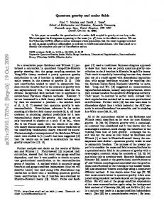
α(a/adisc) 1

0

1 a/adisc

FIG. 1: The correction function (28) as a function of the scale factor (solid line). The asymptotic form (29) for large a is shown by the dashed line. (The sharp cusp, a consequence of the absolute value appearing in (28), is present only for eigenvalues as plotted here, but would disappear for expectation values of the inverse volume operator in coherent states. This cusp will play no role in the analysis of this paper.)

with the scale factor a related to q by q = det(qab ) = a6 . Moreover, in this case the quantum gravitational expectation for α(q), as per Eqs. (B9) and (B10), simplifies: 2  √ (28) α(a) = 8 2(a/adisc )2 (2(a/adisc )2 + 1)1/4 − |2(a/adisc )2 − 1|1/4

where adisc is a scale, determined by the precise discrete quantum state describing an expanding universe at a given time, which provides the fundamental normalization of the scale factor. The function √ is plotted in Fig. 1 One can easily see that α(a) approaches the classical value α = 1 for a ≫ a / 2, while it differs from one for disc √ small a. For a > adisc / 2, the corrections are perturbative in a−1 , 7  adisc 4 α(a) ∼ 1 + +··· . (29) 64 a

This is the first correction in an asymptotic expansion for eigenvalues. If semiclassical states rather than volume eigenstates are used, powers of a−1 in the leading corrections can be smaller. Moreover, the discreteness scale adisc is expected to be not precisely constant but a function of a itself because the underlying spatial discreteness of quantum gravity can be refined dynamically during cosmological evolution [20, 21]. (Indeed, dynamical refinement is also required for several other phenomenological reasons [22–26].) In our following analysis we will thus assume a functional form α(a) = 1 + c(a/a0 )−n

(30)

where we traded the fundamental a normalization by adics for normalization with respect to the present-day value of the scale factor a0 . From the derivation, n is likely to be a small, even integer and c is known to be positive. A precise determination requires knowledge of the dynamical quantum state, which is currently available only in rough effective descriptions. We thus treat the remaining parameters as phenomenological. Energy density and the pressure then are, ignoring the classical interaction term, ρeff = and 3Peff =

ea


2E i α(a) −γDa πξT τ i ξ + πχT τ i χ + i −πξT τ i Da ξ − πχT τ i Da χ − c.c. 6 a

  ea


2E d log α i −γDa πξT τ i ξ + πχT τ i χ + i −πξT τ i Da ξ − πχT τ i Da χ − c.c. . α(a) 1 − 6 a d log a

(31)

(32)

From this, the equation of state w can easily be computed:   1 d log α weff = 1− . 3 d log a

(33)

This quantum gravity correction is independent of the specific matter dynamics as in the classical relativistic case. It results in an equation of state which is linear in ρ, but depends on the geometrical scales (and the Planck length) through α. This is the same general formula derived in [6] for radiation. Thus, on an isotropic background radiation and relativistic fermions are not distinguished by the form of quantum corrections they receive. With the equation of state and the continuity equation a˙ ρ˙ + 3 (ρ + P ) = 0 , a

(34)

where a is the scale factor and the dot indicates a proper time derivative, we can determine energy density as a function of the universe size. We first obtain d log ρ(a) = −3 (1 + w(a)) , d log a explicitly showing the dependence of the equation of state on the scale factor. The solution is  Z  ρ(a) = ρ0 exp −3 (1 + w(a)) d log a ,

(35)

(36)

where ρ0 is the integration constant. Inserting an equation of state of the form (33) we obtain ρ(a) = ρ0 α(a)a−4 .

(37)

For α = 1, we retrieve the classical result ρ(a) ∝ a−4 , but for α 6= 1 loop quantum gravity corrections induced by the discreteness of flux operators are reflected in the evolution of energy density in a Friedmann–Robertson–Walker universe. IV.

EFFECT ON BIG BANG NUCLEOSYNTHESIS

The production of elements in the early universe is highly sensitive to the expansion rate, given by a˙ = a



1/2 8 , πGρ 3

(38)

where ρ is the total density, thus including radiation and fermions. As we have seen here for fermions and in [6] for radiation, the effect of loop quantum gravity corrections is to multiply the effective ρ(a) by a factor α(a). Most importantly, we find that α(a) is the same for both bosons and fermions (up to possible quantization ambiguities), so a separate treatment of the two types of particles in the early universe (as in Ref. [1]) is unnecessary here. In the standard treatment of the thermal history of the universe, the density of relativistic particles (bosons or fermions) is given by ρ=

π2 g∗ T 4 , 30

(39)

where g∗ is the number of spin degrees of freedom for bosons, and 7/8 times the number of spin degrees of freedom for fermions, and T is the temperature, which scales as T ∝ a−1 .

(40)

w = 1/3.

(41)

The equation of state parameter is

Clearly, equations (39)–(41) are inconsistent with equations (33) and (37). There is some ambiguity in determining the correct way to modify the expressions for ρ(T ) and w. We have chosen to assume that the modifications are contained in the gravitational sector, so that the density is given by ρ = α(a)

π2 g∗ T 4 , 30

(42)

with the temperature scaling as in equation (40), and the equation of state w is given by equation (33). This guarantees that the standard continuity equation (34) continues to hold. Note that this is not the only way to incorporate equation (37) into the calculation, but it seems to us the most reasonable way. With these assumptions, we can simply treat α(a) as an effective multiplicative change in the overall value of G. A great deal of work has been done on the use of BBN to constrain changes in G (see, e.g. Refs. [27–31]). The calculation is straightforward, if one has a functional form for the time-variation in G. For the loop quantum gravity corrections considered here, the most reasonable functional form is (30). Note that this expression is by construction valid only in the limit where α(a) − 1 ˙ and the neutron-to-proton ratio ∼ 1 MeV, the weak-interaction rates are faster than the expansion rate, a/a, (n/p) tracks its equilibrium value exp[−∆m/T ], where ∆m is the neutron-proton mass difference. As the universe expands and cools, the expansion rate becomes too fast for weak interactions to maintain weak equilibrium and n/p freezes out. Nearly all the neutrons which survive this freeze-out are converted into 4 He as soon as deuterium becomes stable against photodisintegration, but trace amounts of other elements are produced, particularly deuterium and 7 Li (see, e.g., Ref. [32] for a review). In the standard model, the predicted abundances of all of these light elements are a function of the baryon-photon ratio, η, but any change in G alters these predictions. Prior to the era of precision CMB observations (i.e., before WMAP), Big Bang nucleosynthesis provided the most stringent constraints on η, and modifications to the standard model could be ruled out only if no value of η gave predictions for the light element abundances consistent with the observations. However, the CMB observations now provide an independent estimate for η, which can be used as an input parameter for Big-Bang nucleosynthesis calculations. Copi et al. [30] have recently argued that the most reliable constraints on changes in G can be derived by using the WMAP values for η in conjuction with deuterium observations. The reason is that deuterium can be observed in (presumably unprocessed) high-redshift quasi stellar object (QSO) absorption line systems (see Ref. [33] and references therein), while the estimated primordial 4 He abundance, derived from observations of low metallicity HII regions, is more uncertain (see, for example, the discussion in Ref. [34]). While we agree with the argument of Copi et al. in principle, for the particular model under consideration here it makes more sense to use limits on 4 He than on deuterium, in conjunction with the WMAP value for η. The reason is that the 4 He abundance is most sensitive to changes in the expansion rate at T ∼ 1 MeV, when the freeze-out of the weak interactions determines the fraction of neutrons that will eventually be incorporated into 4 He. Deuterium, in contrast, is produced in Big Bang nucleosynthesis only because the expansion of the universe prevents all of the deuterium from being fused into heavier elements. Thus, the deuterium abundance is most sensitive to the expansion rate at the epoch when this fusion process operates (T ∼ 0.1 MeV). The importance of this distinction with regard to modifications of the standard model was first noted in Ref. [35], and a very nice quantitative analysis was given recently in Ref. [36]. Note that our estimate for the behavior of G(a)/G0 − 1, equation (43), is a steeply decreasing function of a. Thus, the change in the primordial 4 He abundance will always be much larger than the change in the deuterium abundance. Therefore, we can obtain better constraints on this model by using extremely conservative limits on 4 He, rather than by using the more reliable limits on the deuterium abundance. For the same reason, we can ignore any effect on the CMB, since the latter is generated at a much larger value of a, and any change will be minuscule. Hence, we can confidently use the WMAP value for η. WMAP gives [37] −10 η = 6.116+0.197 . −0.249 × 10

(45)

FIG. 2: Solid curve gives upper bound on e c as a function of n, for the assumed form for α: α = 1 + e c/an 10 , where a10 is the value of the scale factor in units for which a10 = 1010 at present.

Because the estimated errors on η are so small, we simply use the central value for η; the bounds we derive on c in equation (30) change only slightly when η is varied within the range given by equation (45). Since c in equations (30) and (43) is thought to be positive, the effect of LQG corrections is to increase the primordial expansion rate, which increases the predicted 4 He abundance. We therefore require an observational upper bound on the primordial 4 He abundance. As noted earlier, this is a matter of some controversy. We therefore adopt the very conservative upper bound recommended by Olive and Skillman [34]: YP ≤ 0.258,

(46)

where YP is the primordial mass fraction of 4 He. For a fixed value of n in equation (43), we determine the largest value of c that yields a primordial 4 He abundance consistent with this upper limit on YP . Since we are essentially bounding the change in G at a/a0 ∼ 10−10 , it is convenient to rewrite equation (30) as α = 1+e c/an10

(47)

where a10 ≡ 1010 (a/a0 ). This upper bound on e c as a function of n is given in Fig. 2. For the special case n = 4, we can use these results to place a bound on adisc in equation (29). We obtain adisc < 2.4 × 10−10 . a0

(48)

This is not a strong bound for the parameters of quantum gravity, but clearly demonstrates that quantum corrections are consistent with successful big bang nuclesynthesis. V.

CONCLUSIONS

Big bang nucleosynthesis is a highly relativistic regime which, to a good approximation, implies identical equations of state for fermions and photons. There are, however, corrections to the simple equation of state w = 13 for fermions even classically. One observation made here is that the interaction term derived in [11] leads to such a correction and might be more constrained by nucleosynthesis than through standard particle experiments [12]. We have not analyzed this further here because more details of the behavior of the fermion current would be required. A second source of corrections arises from quantum gravity. Remarkably, while quantum gravity effects on an isotropic background do correct the equations of state, they do so equally for photons and relativistic fermions.

Initially, this is not expected for both types of fields due to their very different actions. Thus, quantum gravity effects do not spoil the detailed balance required for the scenario to work and bounds from big bang nucleosynthesis obtained so far are not strong. Nevertheless, small deviations in the equations of state and thus energy densities of fermions and radiation are possible. First, there are always quantization ambiguities, and so far we tacitly assumed that the same basic quantization choice is made for the Maxwell and Dirac Hamiltonians. Such ambiguity parameters can be explicitly included in specific formulas for correction functions; see e.g. [19, 38, 39]. Independent consistency conditions for the quantization may at some point require one to use different quantizations for both types of fields, resulting in different quantum corrections and different energy densities. Such conditions can be derived from an analysis of anomaly-freedom of the Maxwell field and fermions coupled to gravity, which is currently in progress. As shown here, if this is the case it will become testable in scenarios sensitive to the behavior of energy density such as big bang nucleosynthesis. Moreover, assuming the same quantization parameters leads to identical quantum corrections for photons and fermions only on isotropic backgrounds. Small-scale anisotropies have different effects on both types of fields and can thus also be probed through their implications on the equation of state. For this, it will be important to estimate the typical size of corrections, which is not easy since it requires details of the quantum state of geometry. The crucial ingredient is the patch size of underlying lattice states. On the other hand, taking a phenomenological point of view allows one to estimate ranges for patch sizes which would leave one in agreement with big bang nucleosynthesis constraints. Acknowledgments

M.B. was supported in part by NSF grants PHY05-54771 and PHY06-53127. R.J.S. was supported in part by the Department of Energy (DE-FG05-85ER40226). Some of the work was done while M.B. visited the Erwin-Schr¨ odingerInstitute, Vienna, during the program “Poisson Sigma Models, Lie Algebroids, Deformations, and Higher Analogues,” whose support is gratefully acknowledged. APPENDIX A: ORIGIN OF TORSION IN THE EINSTEIN-CARTAN ACTION

Here we demonstrate the origin of torsion in the theory of gravity minimally coupled to fermionic matter. The T basic configuration variables in a Lagrangian formulation of fermionic field theory are the Dirac bi-spinor Ψ = (ψ η) T and its complex conjugate Ψ = (Ψ∗ ) γ 0 with γ α being the Minkowski Dirac matrices. We note that ψ and η transform with density weight zero and are spinors according to the fundamental representations of SL (2, C). Then the minimum coupling of gravity to fermions is expressed by the total action (2). Note that we are ignoring the gauge connection required for describing an interaction between charged fermions in the definition of the covariant derivative (4). However, this analysis can be generalized to incorporate such interactions. At this point, it is noteworthy that we intend to use the signature (− + ++) (instead of (+ − −−) which is common in QFT) for both gravity and fermions since this is the signature most prevalent in the literature for canonical gravity. This demands certain modifications in the representations of the Clifford algebra, and it turns out that changing the signature from (+ − −−) to (− + ++) only requires all the Dirac matrices to be multiplied by i (the imaginary unit); see [14] for details. It is easy to see that the covariant derivative in (4) is invariant under the above signature change. Now the variation of the first-order action (2) with respect to the connection gives rise to the equation of motion IJ IJ for the connection. Using δFµν = 2∇[µ δων] and the anticommutator [γK , γ[I γJ] ]+ = −2iǫIJKL γ 5 γ L , we obtain δSG 1 [µ ν] = ∇µ (eeK eL )P KLIJ IJ δωµ 8πG

(A1)

ieeµK δSF 1 = Ψ[γK , γ[I γJ] ]+ Ψ = eeµK ǫIJKL Ψγ 5 γ L Ψ. δωµIJ 8 4

(A2)

Note that the expression (A2) is also invariant under the above signature-change. In other words, the Einstein-Cartan theory before proceeding to a canonical formulation is independent of the signature. Thus we finally obtain the equation of motion for the connection from (A1) and (A2) [µ ν]

∇µ (eeI eJ ) = 2πGeP −1IJ

KL

ν JKL ,

(A3)

µ where JKL := eµI ǫIKLJ J J with the axial fermion current J L = Ψγ 5 γ L Ψ. It is immediate from (A3) that the presence of a fermion field in the coupled action introduces a torsion component in the connection arising from the fermion

current and thus the connection is no longer torsion free, that is, ∇[µ eIν] 6= 0. In terms of connection variables, this issue has been explored in detail in [11–13]. In order to solve for the connection, let us express it in the form IJ ωµIJ = ω e [e]IJ e [e] is the torsion free connection determined by the tetrad and CµIJ is the tetrad projection µ +Cµ , where ω of the contorsion tensor, Cµρσ , i.e., CµIJ = Cµρσ eI[ρ eJσ] . Then the actions of the corresponding covariant derivatives on vectors with internal indices are related as follows:   e µ VI = C J VJ , (A4) ∇µ − ∇ µI

e µ is the covariant derivative compatible with the tetrad, hence having a corresponding connection which is where ∇ torsion-free, and VJ is an internal vector field. Now it follows from (A4) that the two corresponding curvatures satisfy IJ IJ e [µ C IJ + [Cµ , Cν ]IJ Fµν = Feµν + 2∇ ν]

(A5)

where Fe is the curvature of the torsion-free connection. Inserting (A5) in (2) and using (A4), we obtain an action composed of a part in terms of torsion-free variables and an interacting fermion contribution due to torsion: S [e, ω, Ψ] = SG [e, ω e ] + SF [e, ω e , Ψ] + Sint [e, C, Ψ] Z Z h i 1 i e µ Ψγ I eµ Ψ e µΨ − ∇ = d4 x eeµI eνJ P IJKL FeµνKL (e ω) + d4 x e Ψγ I eµI ∇ I 16πG M 2 M Z Z 1 1 d4 x eeµI eνJ P IJKL [Cµ , Cν ]KL + d4 x eeµI Cµ JK ǫI JKL J L. + 16πG M 4 M

(A6)

Notice that the middle term on the right hand side in (A5) is ignored since it can be expressed as a total derivative and therefore does not contribute to the variation. The first two terms are just the torsion-free Holst and Dirac action while the last two terms include torsion. Now, with the use of (A4), the contorsion tensor CµI J can be solved by expressing the equation of motion (A3) as   γ2 1 M N ν [µ ν] K [µ ν] K [µ ν] KL ν ∇µ (eeI eJ ) = eCµI eK eJ + eCµJ eI eK = 2πGe 2 (A7) ǫ eK JL − δ[I δJ] eM JN . γ + 1 IJ γ From this, the following equation can be obtained by contracting equation (A7) with eIν eJρ : CµJ K eµK eJρ := SµJ µ eJρ = 0.

(A8)

Since the tetrads eIµ are invertible, the above equation implies that SµJ µ = CµJ K eµK = 0. Upon inserting this solution in equation (A7) the equation of motion becomes   1 M N ν γ2 δJ] eM JN . ǫIJ KLeνK JL − δ[I (A9) eµI SµJ ν − eµJ SµI ν = 2S[IJ]ν = 4πG 2 γ +1 γ Again contracting with eM ν , we have S[IJ]

M

γ2 = 2πG 2 γ +1



ǫIJ

ML

1 M JL − η[I JJ] γ



.

(A10)

Notice that CµIJ = Cµ[IJ] implies that SIJK = SIJ M ηM K = eµI CµJK = SI[JK] . The following combination of the cyclic permutations of the indices I, J, and K finally yields the expression for CµIJ :   2 γ2 ǫIJKL J L − ηI[J JK] . (A11) eµI CµJK = S[IJ]K − S[JK]I + S[KI]J = SIJK = 2πG 2 γ +1 γ Note that the contorsion tensor CµIJ depends on the Immirzi parameter γ. The following useful identities can be derived after a straightforward but lengthy calculation using the above expression for CµIJ : 1 3πG γ 2 eµI eνJ P IJKL [Cµ, Cν ]KL = JL J L , 16πG 2 γ2 + 1 1 µ 6πG γ 2 eI Cµ JK ǫI JKL J L = − JLJ L . 4 2 γ2 + 1

(A12)

Finally, upon inserting (A12) in (A6), we obtain a simple interacting term in the total action: S [e, ω, Ψ] = SG [e, ω e ] + SF [e, ω e , Ψ] + Sint [e, C, Ψ] Z Z i h 1 i e µΨ − ∇ e µ Ψγ I eµ Ψ = d4 x eeµI eνJ P IJKL FeµνKL (e ω) + d4 x e Ψγ I eµI ∇ I 16πG M 2 M Z 2 3κ γ − d4 x e(Ψγ5 γL Ψ)(Ψγ 5 γ L Ψ) . 16 γ 2 + 1 M

(A13)

The last term in this simplified action describes a four-fermion interaction mediated by non-propagating torsion. APPENDIX B: ELEMENTS OF LOOP QUANTUM GRAVITY

We collect the basic formulas required to compute quantum corrections in loop quantum cosmology, referring to [6, 19] for further details. We can restrict our attention to perturbative regimes around a spatially flat isotropic solution where one can choose the canonical variables to be given by functions (˜ pI (x), ˜kJ (x)) which determine a densitized triad by Eia = p˜(i)(x)δia and extrinsic curvature by Kai = k˜(i)(x)δai . This diagonalization implies strong simplifications in the explicit evaluation of formulas [40, 41]. Any state is associated with a spatial lattice with U(1) elements ηv,I attached to its links ev,I starting at a vertex v and pointing in a direction along a translation generator XIa of the homogeneous background. The U(1) elements ηv,I appear as matrix elements in SU(2) holonomies hv,I = Reηv,I + 2τI Imηv,I and represent the connection, while fluxes Fv,I are used as independent variables for the momenta. An orthonormal basis of the quantum Hilbert space Q µv,I is given by functionals | . . . , µv,I , . . .i = v,I ηv,I , for all possible choices of µv,I ∈ Z. Together with basic operators, which are represented as holonomies ηˆv,I | . . . , µv ′,J , . . .i = | . . . , µv,I + 1, . . .i

(B1)

for each pair (v, I), and fluxes Fˆv,I | . . . , µv ′,J , . . .i = 2πγℓ2P (µv,I + µv,−I )| . . . , µv ′,J , . . .i , (B2) √ this defines the basic quantum representation. Here, ℓP = ~G is the Planck length and a subscript −I means that the edge preceding the vertex v in the chosen orientation is taken. For effective equations, one important step in addition to computing expectation values of operators is the introduction of a continuum limit. This relates holonomies ηv,I = exp(i ∫ dtγ k˜I /2) ≈ exp(iℓ0 γ k˜I (v + I/2)/2)

(B3)

ev,I

to continuum fields k˜I through mid-point evaluation (denoted by v + I/2), and similarly for fluxes Z Fv,I = p˜I (y)d2 y ≈ ℓ20 p˜I (v + I/2) .

(B4)

Sv,I

Here, ℓ0 is the coordinate length of lattice links, which enters the continuum approximation since we are integrating P Q3 q ˆ classical fields in holonomies and fluxes. From flux operators one defines the volume operator V = v I=1 |Fˆv,I |, p p R P P p using the classical expression V = d3 x |p˜1 p˜2 p˜3 | ≈ v ℓ30 |p˜1 p˜2 p˜3 | = v |p1 p2 p3 |. With (B2), its eigenvalues are V ({µv,I }) =

3 q
XY 2 3/2 |µv,I 2πγℓP v I=1

+ µv,−I | .

(B5)

The volume operator is central for inverse triad corrections because inverse densitized triads, or a co-triad, can be quantized using relations such as {Aia , Vvr } = 4πγG rVvr−1 eia

(B6)

for 0 < r < 2. Even though an inverse power of volume, together with a co-trad, occurs on the right hand side, the left hand side can be quantized directly in terms of the volume operator, using holonomies for connection components, and turning the Poisson bracket into a commutator [16, 42]. Such a quantization leads to r−1 i V\ eI = v

−2 8πirγℓ2P ℓ0

X

σ∈{±1}

1 ˆ (r) ˆr ˆ (r) )δ i =: 1 Cˆ (r) δ i σ tr(τ i hv,σI [h−1 (B − B v,σI , V v ]) = v,−I (I) 2ℓ0 v,I ℓ0 v,I (I)

(B7)

ˆ (r) is, after taking the trace where, for symmetry, we use both edges touching the vertex v along direction XIa and B v,I in (B7),   1 ˆ (r) := (B8) sv,I Vˆvr cv,I − cv,I Vˆvr sv,I B v,I 4πiγG~r with cv,I =

1 ∗ (ηv,I + ηv,I ) 2

and

sv,I =

1 ∗ (ηv,I − ηv,I ). 2i

As in [19] effects of the quantization of triad (metric) coefficients are included by inserting correction functions in the classical Hamiltonian which follow, e.g., from the eigenvalues [19]   (1/2) Cv,I ({µv ′ ,I ′ }) = 2(2πγℓ2P )−1/4 |µv,J + µv,−J |1/4 |µv,K + µv,−K |1/4 |µv,K + µv,−K + 1|1/4 − |µv,K + µv,−K − 1|1/4

(B9) (1/2) (where indices J and K are defined such that ǫIJK 6= 0) of operators Cˆv,I . Although for large µv,I these eigenvalues approach the function p Q3 |µv,K + µv,−K | (1/2) (1/2) 2 −1/2 K=1 Cv,I ({µv ′ ,I ′ })Cv,J ({µv ′ ,I ′ }) ∼ (2πγℓP ) |µv,I + µv,−I ||µv,J + µv,−J | p √ expected classically for qIJ / q = |p1 p2 p3 |/pI pJ with a densitized triad Eia = p(i) δia and using the relation (B2) between labels and flux components, they differ for values of µv,I closer to one. This deviation can, for an isotropic background, be captured in a single correction function p 2πγℓ2P (µv,I + µv,−I )2 1 X (1/2) 2 αv,K = (B10) Cv,I ({µv ′ ,I ′ }) · Q3 p 3 |µv,J + µv,−J | J=1 I

which would equal one in the absence of quantum corrections. This is indeed approached in the limit where all µv,I ≫ 1, but for any finite values there are corrections. If all µv,I > 1 one can directly check that corrections are positive, i.e. αv,K > 1 in this regime. Expressing the labels in terms of the densitized triad through fluxes (B2) results in functionals α[pI (v)] = αv,K (4πγℓ2P µv,I )

(B11)

which enter effective Hamiltonians.

[1] J. Barrow and R. J. Scherrer, Do Fermions and Bosons Produce the Same Gravitational Field?, Phys. Rev. D 70 (2004) 103515, [astro-ph/0406088] [2] M. Bojowald, Loop Quantum Cosmology, Living Rev. Relativity 8 (2005) 11, [gr-qc/0601085], http://relativity.livingreviews.org/Articles/lrr-2005-11/ [3] C. Rovelli, Quantum Gravity, Cambridge University Press, Cambridge, UK, 2004 [4] A. Ashtekar and J. Lewandowski, Background independent quantum gravity: A status report, Class. Quantum Grav. 21 (2004) R53–R152, [gr-qc/0404018] [5] T. Thiemann, Introduction to Modern Canonical Quantum General Relativity, [gr-qc/0110034] [6] M. Bojowald and R. Das, Radiation equation of state and loop quantum gravity corrections, Phys. Rev. D 75, 123521 (2007). [7] F. W. Hehl, P. von der Heyde, G. D. Kerlick and J. M. Nester, General relativity with spin and torsion: Foundations and prospects, Rev. Mod. Phys. 48 (1976) 393–416

[8] J. F. Barbero G., Real Ashtekar Variables for Lorentzian Signature Space-Times, Phys. Rev. D 51 (1995) 5507–5510, [gr-qc/9410014] [9] G. Immirzi, Real and Complex Connections for Canonical Gravity, Class. Quantum Grav. 14 (1997) L177–L181 [10] S. Holst, Barbero’s Hamiltonian derived from a generalized Hilbert-Palatini action, Phys. Rev. D 53 (1996) 5966–5969, [gr-qc/9511026] [11] A. Perez and C. Rovelli, Physical effects of the Immirzi parameter, Phys. Rev. D 73 (2006) 044013, [gr-qc/0505081] [12] L. Freidel, D. Minic, and T. Takeuchi, Quantum Gravity, Torsion, Parity Violation and all that, Phys. Rev. D 72 (2005) 104002, [hep-th/0507253] [13] S. Mercuri, Fermions in Ashtekar-Barbero Connections Formalism for Arbitrary Values of the Immirzi Parameter, Phys. Rev. D 73 (2006) 084016, [gr-qc/0601013] [14] M. Bojowald and R. Das, Canonical Gravity with Fermions [15] T. Thiemann, Kinematical Hilbert Spaces for Fermionic and Higgs Quantum Field Theories, Class. Quantum Grav. 15 (1998) 1487–1512, [gr-qc/9705021] [16] T. Thiemann, QSD V: Quantum Gravity as the Natural Regulator of Matter Quantum Field Theories, Class. Quantum Grav. 15 (1998) 1281–1314, [gr-qc/9705019] [17] M. Bojowald and A. Skirzewski, Effective Equations of Motion for Quantum Systems, Rev. Math. Phys. 18 (2006) 713–745, [math-ph/0511043] [18] M. Bojowald and A. Skirzewski, Quantum Gravity and Higher Curvature Actions, Int. J. Geom. Math. Mod. Phys. 4 (2007) 25–52, [hep-th/0606232] [19] M. Bojowald, H. Hern´ andez, M. Kagan, and A. Skirzewski, Effective constraints of loop quantum gravity, [gr-qc/0611112] [20] M. Bojowald, Loop quantum cosmology and inhomogeneities, Gen. Rel. Grav. 38 (2006) 1771–1795, [gr-qc/0609034] [21] M. Bojowald, The dark side of a patchwork universe, Gen. Rel. Grav. (2007), to appear, [arXiv:0705.4398] [22] A. Ashtekar, T. Pawlowski and P. Singh, Quantum Nature of the Big Bang: Improved dynamics, Phys. Rev. D 74 (2006) 084003, [gr-qc/0607039] [23] M. Bojowald, D. Cartin and G. Khanna, Lattice refining loop quantum cosmology, anisotropic models and stability, Phys. Rev. D 76 (2007) 064018, [arXiv:0704.1137] [24] W. Nelson and M. Sakellariadou, Lattice Refining Loop Quantum Cosmology and Inflation, Phys. Rev. D 2007, to appear, [arXiv:0706.0179] [25] W. Nelson and M. Sakellariadou, Lattice Refining LQC and the Matter Hamiltonian, arXiv:0707.0588 [26] M. Bojowald and G. M. Hossain, Quantum gravity corrections to gravitational wave dispersion, arXiv:0709.2365 [27] J.D. Barrow, Mon. Not. R. Astr. Soc. 184, 677 (1978). [28] J. Yang, D.N. Schramm, G. Steigman, and R.T. Rood, Astrophys. J. 227, 697 (1979). [29] F.S. Accetta, L.M. Krauss, and P. Romanelli, Phys. Lett. B 248, 146 (1990). [30] C.J. Copi, A.N. Davis, and L.M. Krauss, Phys. Rev. Lett. 92 (2004) 171301. [31] T. Clifton, J.D. Barrow, and R.J. Scherrer, Phys. Rev. D 71 (2005) 123526. [32] K.A. Olive, G. Steigman, and T.P. Walker, Phys. Rep. 333 (2000) 389. [33] D. Kirkman, D. Tytler, N. Suzuki, J.M. O’Meara, and D. Lubin, Ap.J. Suppl. 149 (2003) 1. [34] K.A. Olive and E.D. Skillman, Ap.J, 617 (2004) 29. [35] E.W. Kolb and R.J. Scherrer, Phys. Rev. D 25 (1982) 1481. [36] C. Bambi, M Giannotti, and F.L. Villante, Phys. Rev. D 71 (2005) 123524. [37] D.N Spergel, et al., astro-ph/0603449. [38] M. Bojowald, Quantization ambiguities in isotropic quantum geometry, Class. Quantum Grav. 19 (2002) 5113–5130, [gr-qc/0206053] [39] M. Bojowald, Loop Quantum Cosmology: Recent Progress, In Proceedings of the International Conference on Gravitation and Cosmology (ICGC 2004), Cochin, India, Pramana 63 (2004) 765–776, [gr-qc/0402053] [40] M. Bojowald, Loop Quantum Cosmology: I. Kinematics, Class. Quantum Grav. 17 (2000) 1489–1508, [gr-qc/9910103] [41] M. Bojowald, Spherically Symmetric Quantum Geometry: States and Basic Operators, Class. Quantum Grav. 21 (2004) 3733–3753, [gr-qc/0407017] [42] T. Thiemann, Quantum Spin Dynamics (QSD), Class. Quantum Grav. 15 (1998) 839–873, [gr-qc/9606089]