Dirac Fields in Loop Quantum Gravity and Big Bang Nucleosynthesis

Dirac Fields in Loop Quantum Gravity and Big Bang Nucleosynthesis Martin Bojowald Institute for Gravitation and the Cosmos, The Pennsylvania State University, 104 Davey Lab, University park, PA

16802

Rupam Das Department of Physics and Astronomy, Vanderbilt University, Nashville, TN 37235 and Institute for Gravitation and the Cosmos, The Pennsylvania State University, 104 Davey Lab, University park, PA

16802

Robert J. Scherrer

arXiv:0710.5734v2 [astro-ph] 19 Mar 2008

Department of Physics and Astronomy, Vanderbilt University, Nashville, TN

37235

Big Bang nucleosynthesis requires a fine balance between equations of state for photons and relativistic fermions. Several corrections to equation of state parameters arise from classical and quantum physics, which are derived here from a canonical perspective. In particular, loop quantum gravity allows one to compute quantum gravity corrections for Maxwell and Dirac fields. Although the classical actions are very different, quantum corrections to the equation of state are remarkably similar. To lowest order, these corrections take the form of an overall expansion-dependent multiplicative factor in the total density. We use these results, along with the predictions of Big Bang nucleosynthesis, to place bounds on these corrections and especially the patch size of discrete quantum gravity states. PACS numbers: 04.20.Fy, 04.60.Pp,98.80.Ft

I.

INTRODUCTION

Much of cosmology is well-described by a space-time near a spatially isotropic Friedmann–Robertson–Walker models with line elements   dr2 2 2 2 2 ds2 = −dτ 2 + a(τ )2 + r (dϑ + sin ϑdϕ ) (1) 1 − kr2 where k = 0 or ±1, sourced by perfect fluids with equations of state P = wρ. Such an equation of state relates the matter pressure P to its energy density ρ and captures the thermodynamical properties in a form relevant for isotropic space-times in general relativity. Often, one can assume the equation of state parameter w to be constant during successive phases of the universe evolution, with sharp jumps between different phases such as w = −1 during inflation, followed by w = 31 during radiation domination and w = 1 during matter domination. Observationally relevant details can depend on the precise values of w at a given stage, in particular if one uses an effective value describing a mixture of different matter components. For instance, during big bang nucleosynthesis one is in a radiation dominated phase mainly described by photons and relativistic fermions. Photons, according to Maxwell theory, have an exact equation of state parameter w = 13 as a consequence of conformal invariance of the equations of motion (such that the stress-energy tensor is trace-free). For fermions the general equation of state is more complicated and non-linear, but can in relativistic regimes be approximately given by the same value w = 31 as for photons. In contrast to the case of Maxwell theory, however, there is no strict symmetry such as conformal invariance which would prevent w to take a different value. It is one of the main objectives of the present paper to discuss possible corrections to this value. For big bang nucleosynthesis, it turns out, the balance between fermions and photons is quite sensitive. In fact, different values for the equation of state parameters might even be preferred phenomenologically [1]. One possible reason for different equations of state could be different coupling constants of bosons and fermions to gravity, for which currently no underlying mechanism is known. In this paper we will explore the possibility whether quantum gravitational corrections to the equations of state can produce sufficiently different values for the equation of state parameters. In fact, since the fields are governed by different actions, one generally expects different, though small, correction terms which can be of significance in a delicate balance. Note that we are not discussing ordinary quantum corrections of quantum fields on a classical background. Those are expected to be similar for fermions and radiation in relativistic regimes. We rather deal with quantum gravity corrections in the coupling of the fields to the space-time metric, about which much less is known a priori. Thus, different proposals of quantum gravity may differ at this stage, providing possible tests. An approach where quantum gravitational corrections can be computed is loop quantum cosmology [2], which specializes loop quantum gravity [3, 4, 5] to cosmological regimes. In such a canonical quantization of gravity,

2 equations of state must be computed from matter Hamiltonians rather than covariant stress-energy tensors. Quantum corrections to the underlying Hamiltonian then imply corrections in the equation of state. This program was carried out for the Maxwell Hamiltonian in [6], and is done here for Dirac fermions. There are several differences between the treatment of fermions and other fields, which from the gravitational point of view are mainly related to the fact that fermions, in a first order formulation, also couple to torsion and not just the curvature of space-time. After describing the classical derivation of equations of state as well as steps of a loop quantization and its correction terms, we use big bang nucleosynthesis constraints to see how sensitively we can bound quantum gravity parameters. We have aimed to make the paper nearly self-contained and included some of the technical details. Secs. III on the canonical formulation of fermions, IV on quantum corrections from loop quantum gravity and V on the analysis of big bang nucleosynthesis can, however, be read largely independently of each other by readers only interested in some of the aspects covered here. We will start with general remarks on the physics underlying the problem. II.

THE PHYSICAL SETTING

Big bang nucleosynthesis happens at energy scales EBBN ∼ MeV which are large, but still tiny compared to the Planck energy MP . Also the universe has already grown large compared to the Planck length ℓP at this stage, and space-time curvature is small. One may thus question why quantum gravity should play any role. There is certainly a fine balance required for successful big bang nucleosynthesis, but the expected quantum gravity terms of the order E/MP , obtained based on dimensional arguments, would have no effect. However, dimensional arguments do not always work, in particular if more than two parameters LI of the same dimension, or any large Q dimensionlessPnumbers are involved. Then, precise calculations have to be done to determine which geometric means I LxI I with I xI = 0 may appear as coefficients, or which powers of dimensionless numbers occur as factors of correction terms. In loop quantum gravity, we are in such a situation: there is the macroscopic length scale L, which in√our case we can take as the typical wave length of fields during nucleosynthesis, and also the Planck length ℓP = G~ which arises due to the presence of Newton’s constant G and Planck’s constant ~. In addition, there is a third and in general independent scale ℓ given by the microscopic size of elementary spatial patches in a quantum gravity state. This is a new feature of the fundamentally discrete theory, for which the precise state of quantum gravity plays an important role. Although ℓ must be proportional to the Planck length, its specific value for a given state can differ numerically. Then, a detailed calculation must show how L, ℓ and ℓP appear in quantum gravity corrections and which numerical values may arise. Alternatively, one can work with only two length scales, L and ℓP , but one has to deal with a large dimensionless parameter N given by the number of discrete patches of the underlying state in the volume considered, for instance a volume of the size L3 such that N = L3 /ℓ3 . Examples of cosmological phenomena are known where this does play a role for quantum gravity corrections [7, 8], and here we analyze which features arise in the presence of fermions and especially for big bang nucleosynthesis. There are precedents where such considerations have played important roles. Best known is the evidence for the atomic nature of matter derived by Einstein from the phenomenon of Brownian motion. Also here, there are several orders of magnitude between the expected size of molecules and the resolution of microscopes at that time. However, there is also a large number of molecules which by their sheer number can and do leave sizeable effects on much larger suspended particles. There is, of course, never a guarantee that something analogous has to happen elsewhere. But this is to be checked by calculations and cannot always be ruled out based only on dimensional arguments. We can use the result of corrections to the equation of state of radiation derived in [6], but a new analysis is required for fermions and their specific action. Even in relativistic regimes, the coupling of fermions to gravity differs from other fields, e.g. by torsion contributions which arise already from the kinetic term of the Dirac action. One could thus expect that quantum corrections for fermions differ from those to radiation and thus, by throwing off the balance during nucleosynthesis, possibly enhance the effect of quantum gravity corrections. Whether or not this happens cannot be decided without detailed calculations as they are reported and applied here. III.

CANONICAL FORMULATION OF DIRAC FERMIONS

For fermions, one has to use a tetrad eIµ rather than a space-time metric gµν , which are related by eIµ eIν = gµν , in order to formulate an action with the appropriate covariant derivative of fermions. This naturally leads one to a first-order formalism of gravity in which the basic configuration variables are a connection 1-form and the tetrad. In vacuum the connection would, as a consequence of field equations, be the torsion-free spin connection compatible with the tetrad. In the presence of matter fields which couple directly to the connection, such as fermions, this is no longer the case and there is torsion [9, 16, 17].

3 A.

Non-minimally Coupled Einstein-Dirac Action

A canonical analysis of gravity minimally coupled to fermions is presented in detail in [17]. In [16], a non-minimally coupled action is proposed in order to eliminate violations of parity. Here, we first present a general canonical analysis providing a consistent canonical formulation for all coupling parameters. At the end of this section, we briefly comment on parity which plays a role in this context. The basic configuration variables in a Lagrangian formulation of fermionic field theory are the Dirac bi-spinor Ψ = (ψ η)T and its adjoint Ψ = (Ψ∗ )T γ 0 with γ α being the Minkowski Dirac matrices. The 2-component SL(2, C)spinors ψ and η will be used later on in a Hamiltonian decomposition of the action. Being interested in applications to highly relativistic regimes, we only deal with massless fermions. Their non-minimal coupling to gravity can then be expressed, in the notation of [16], by the total action S [e, ω, Ψ] = SG [e, ω] + SF [e, ω, Ψ] Z 1 = d4 x eeµI eνJ P IJKL FµνKL (ω) 16πG M       Z i 1 i d4 x e Ψγ I eµI 1 − γ5 ∇µ Ψ − ∇µ Ψ 1 − γ5 γ I eµI Ψ , + i 2 M α α

(2)

where α is the parameter for non-minimal coupling and minimal coupling is reproduced for α → ∞. The action is composed of the matter contribution SF resulting from the fermion field and the gravitational contribution SG expressed in terms of   1 ǫIJKL 1 ǫIJ KL γ2 KL [I J] [K L] P IJKL = δK δL − δI δJ + (3) , P −1IJ = 2 γ 2 γ +1 γ 2 where γ is the Barbero–Immirzi parameter [10, 11]. The specific form of the gravitational action is the one given by Holst [12], formulated in terms of a tetrad field eµI with inverse eIµ , whose determinant is e. (Thus, the space-time metric is gµν = eIµ eIν . For all space-time fields, I, J, . . . = 0, 1, 2, 3 denote internal Lorentz indices and µ, ν, . . . = 0, 1, 2, 3 space-time indices.) The Lorentz connection IJ KL IJ ωµIJ in this formulation is an additional field independent of the triad, and Fµν (ω) = 2∂[µ ων] + [ωµ , ων ] is its curvature. It also determines the covariant derivative ∇µ of Dirac spinors by 1 ∇µ ≡ ∂µ + ωµIJ γ[I γJ] 4

,

[∇µ , ∇ν ] =

1 IJ F γ[I γJ] 4 µν

(4)

in terms of Dirac matrices γI (which will always carry an index such that no confusion with the Barbero–Immirzi parameter γ can arise). B.

Dirac Hamiltonian

As usually, a Hamiltonian formalism of gravity requires a space-time foliation Σt : t = const such that one can introduce fields and their rates of change, which will provide canonical variables. This is done by referring to a time function t as well as a time evolution vector field tµ such that tµ ∇µ t = 1. Rates of change of spatial fields will then be associated with their derivatives along ta . For convenience, one decomposes tµ into normal and tangential parts with respect to Σt by defining the lapse function N and the shift vector N a such that tµ = N nµ + N µ with N µ nµ = 0. Here, nµ is the unit normal vector field to the hypersurfaces Σt . The space-time metric gµν induces a spatial metric qµν (t) on Σt by the formula gµν = qµν − nµ nν . This is one of the basic fields of a canonical formulation, and its momentum will be related to q˙ab defined as the Lie derivative of qab along ta . Since contractions of qµν and N µ with the normal nµ vanish, they give rise to spatial tensors qab and N a . In our case, we are using a tetrad formulation, where eIµ provides a map from the tangent space of space-time to an internal Minkowski space. The space-time foliation thus requires an associated space-time splitting of the Minkowski space. This takes the form of a partial gauge fixing on the internal vector fields of the tetrad: the directions (or rather boosts) of tetrad fields can no longer be chosen arbitrarily. Instead, we decompose the tetrad into a fixed internal unit time-like vector field and a triad on the space Σt . We choose the internal vector field to be constant, nI = −δI,0 with nI nI = −1. Then, we allow only those tetrads which are compatible with the fixed nI in the sense that na = nI eaI is the unit normal to the given foliation. This implies that eaI = EIa − na nI with EIa na = EIa nI = 0 so that EIa is a spatial triad.

4 Now, using eaI = EIa − na nI with nI = −δI,0 and na = N −1 (ta − N a ) we can decompose the non-minimally coupled Dirac action and write it in terms of spatial fields only:       Z √ i i i I a −1 a a 4 I a −1 a a d x N q Ψγ (EI + N (t − N )) 1 − γ5 ∇a Ψ − ∇a Ψ 1 − γ5 γ (EI + N (t − N ))Ψ , SDirac = 2 M α α (5) √ where the space-time determinant is factorized as e = N q with the determinant q of the spatial metric. These terms can be decomposed into several terms containing the SL(2, C)-spinors ψ and η instead of the Dirac spinor Ψ:  i √  i √ a N qn (Ψγ 0 ∇a Ψ − c.c.) + N Eia (Ψγ i ∇a Ψ − c.c.) = q − 12 i(ψ † ψ˙ + η † η˙ − c.c.) + 41 ǫmnk ωt mn J k 2 2
√ √ − qN a − 21 i(ψ † ∂a ψ + η † ∂a η − c.c.) + 14 ǫmnk ωamn J k − N qEia − 21 i(−ψ † σ i ∂a ψ + η † σ i ∂a η − c.c.)
− 41 ǫi mn ωamn (ψ † ψ − η † η) + 12 ǫi mn ωam0 J n ,

(6)

and similarly an expansion of the terms involving the non-minimal coupling parameter α in the action (5) gives

1 √ q((ta − N a ) Ψγ 0 γ5 ∇a Ψ − ∇a Ψγ5 γ 0 Ψ + N Eia Ψγ i γ5 ∇a Ψ − ∇a Ψγ5 γ i Ψ ) 2α 1 √ a q(t − N a )(ψ † ∂a ψ − η † ∂a η + (∂a ψ † )ψ − (∂a η † )η − ωaj0 J j ) = 2α
N√ a † i qEi ψ σ ∂a ψ + η † σ i ∂a η + (∂a ψ † )σ i ψ + (∂a η † )σ i η + ωaik Jk − ωai0 J0 , + 2α

(7)

where c.c. denotes complex conjugation and we have introduced the fermion current J k := ψ † σ k ψ + η † σ k η and the time component J0 := ψ † ψ − η † η. Details of this calculation as well as the corresponding canonical decompositions of the gravitational part can be found in [17]. We also refer to [17] for the definition of canonical gravitational variables as they appear also in the matter action. In terms of the connection components ωµIJ in Eq. (4), we define 1 Γib := − ǫi jk ωbjk 2

,

Kbi := −ωbi0

(8)

and the Ashtekar–Barbero connection [10, 13] 1 Aia := Γia + γKai = − ǫi kl ωakl − γωai0 2

(9)

with the Barbero–Immirzi parameter γ [11]. This connection is important because it provides a convenient canonical structure with Poisson brackets {Aia (x), Ejb (y)} = 8πγGδab δji δ(x − y)

(10)

√ with the densitized triad Ejb := qEjb . Moreover, following the steps presented in [17], it is straightforward to show that the torsion contribution to the spin connection Γ is given by     γκ γ j k l 1 j j 0 Ca := . (11) 1− ǫ kl ea J − γ + e J 4(1 + γ 2 ) α α a e i + C i , with Γ e i being the torsion-free spin connection compatible with the co-triad One can then show that Γia = Γ a a a i ea . For a fixed value of γ, the above equation for torsion reduces to that for minimal coupling as α → ∞. As noted in [16], based on a Lagrangian analysis, another interesting case is α = γ, which reduces Caj to − κ4 eia J 0 , making torsion γ-independent. The non-minimal coupling is important for the behavior of the action under parity reversal, and it is the value α = γ which provides parity invariance of the combined system of gravity and fermions. This may seem surprising because neither vacuum gravity nor the minimal Dirac action on a fixed background violate parity, and thus the extra term of non-minimal coupling seems to introduce parity violation. As [16] in the Lagrangian picture and [17] in the Hamiltonian picture show, however, the torsion introduced by coupling fermions to gravity also introduces parity violation in the Holst action, which has to be canceled by the additional term of non-minimal coupling. (The action with minimal coupling was called “not fully consistent” in [16], while our analysis is consistent for any value of

5 α. To avoid potential confusion, one should first note that [16] starts from the Einstein–Cartan action with minimal coupling, not directly from a Holst action as here. Parity properties are different in both cases, and the observation of [16] refers only to this behavior. The Holst action with minimal coupling would indeed be inconsistent with parity preservation, but it does not present an inconsistency of the overall framework unless one explicitly requires parity preservation. In fact, parity violation is expected at the onset of BBN due to weak interactions. Anyway, the following discussion of our paper can remain unchanged for different values of α and thus applies directly to the parity preserving case.) Upon inserting (11) in (6) and (7), the action (5) takes the form    Z Z 
√ 1 j0 i θL (ψ † ψ˙ − η˙ † η) − θR (ψ˙ † ψ − η † η) ˙ − 14 ǫmnk ωt mn J k + ωt Ji d3 x q SDirac Pia , Γia , ψ, ψ † , η, η † = − dt 2α Σ   t  
1 1 √ −N a i θL (ψ † Da ψ − Da ηη) + θR (η † Da η − Da ψψ) − γ+ Kai qJi 2 α   
1 1 γ+ Eia Kai J 0 +N Eia iθL (ψ † σ i Da ψ + Da ησ i η) − iθR (η † σ i Da η + Da ψσ i ψ) − 2 α   1 γ n + ǫlkn Kal Eka 1 − , (12) J 2 α where θL := 21 (1 + αi ), θR := 12 (1 − αi ) and we have used the covariant derivatives, Da = ∂a + Ala τl , related to the Ashtekar-Barbero connection, and τl = − 12 iσl . The first part of the action in this form shows that momenta of the √ √ fermion field are πξ = −iξ † of ξ = 4 qψ and πχ = −iχ† of χ = 4 qη. Here, we are using half-densitized spinor fields to avoid complex-valued canonical variables [18]. R Moreover, the action provides the Hamiltonian H = d3 xN (x)δS/δN . Together with fermion dependent terms resulting from the gravitational action, this provides derivative terms and self-interaction terms in the Hamiltonian  Z

βE a 2E i d3 xN − √ i Da πξT τ i ξ + πχT τ i χ − i √ a θL πξT τ i Da ξ − θR πχT τ i Da χ − c.c. HDirac = (13) q q Σt    γ γ T 3γκ  γκβ T T T T T T l T l 2 3 − 1 − (π ξ − π χ)(π ξ − π χ) (π τ ξ + π τ χ)(π τ ξ + π τ χ) + + 2γ + √ √ ξ χ ξ χ ξ l χ l ξ χ 2 q(1 + γ 2 ) α 8α q α with β := γ + α1 . The top line of this expression is the most important one because its derivative terms are dominant in relativistic regimes. In addition to those, we highlight the presence of four-fermion interactions in the second line, which we summarize as  γκβ  γ γ T 3γκ  T T T l T l 2 B := 3 − 1 − (πξ ξ − πχT χ)(πξT ξ − πχT χ) (14) (π τ ξ + π τ χ)(π τ ξ + π τ χ) + + 2γ l l ξ χ ξ χ 2(1 + γ 2 ) α 8α α as it multiplies q −1/2 . C.

Equation of state

From the Hamiltonian we can determine energy and pressure and formulate the equation of state. The matter Hamiltonian is directly related to energy density by 1 δHDirac ρ= √ q δN and thus, from (13), the energy density is  

β B 2Eia − Da πξT τ i ξ + πχT τ i χ + i −θL πξT τ i Da ξ + θR πχT τ i Da χ − c.c. + ρ = q 2 q

(15)

(16)

The canonical formula for pressure is

P =−

δHDirac 2 √ Eia 3N q δEia

(17)

6 as shown by a straightforward adaptation of the calculation done in [6] for metric variables. Now using the functional derivative p δ q(x) 1 = eia δ(x − y) , (18) δEia (y) 2 and thus δ δEjb (y)

2Eia (x) p q(x)

!

1 = √ (2δba δij − eai ejb )δ(x − y) , q

and inserting (19) in (17), we obtain the pressure  

β B 2Eia − Da πξT τ i ξ + πχT τ i χ + i −θL πξT τ i Da ξ + θR πχT τ i Da χ − c.c. + P = 3q 2 q

(19)

(20)

This results in an equation of state

wDirac =

P 1 2B = − . ρ 3 3ρ

(21)

In relativistic regimes, the kinetic term involving partial derivatives ∂a contained in Da is dominant, which leaves us with an equation of state w=

P 1 = +ǫ ρ 3

(22)

whose leading term agrees with the parameter for a Maxwell field. But there are clearly correction terms for fermions already in the classical first order theory. They do not arise for the Maxwell field, implying a difference in the coupling to gravity due to torsion, which is present even in relativistic regimes. The order of magnitude of the additional term depends on the fermion current density and is thus not expected to be large unless regimes are very dense. We will not consider this correction further in this article, but highlight its role as a consequence of torsion. In addition, the canonical analysis performed here provides the stage for a quantization of the theory, resulting in further correction terms from quantum gravity as they occur even for the Maxwell field [6]. Their magnitudes must also be extracted and then compared for the different fields. IV.

QUANTUM CORRECTIONS

We are now in a position to derive the form of quantum gravity corrections for fermion fields in an explicit scenario of quantum gravity, completing the program of Sec. II. We will not require the quantized dynamics of gravity, which makes our aim feasible. But we do need to know how the triad is quantized because it appears in the Dirac Hamiltonian. It appears as a basic variable in the Poisson relations (10), together with the Ashtekar–Barbero connection Aia . Loop quantum gravityR [3, 4, 5] proceeds by forming a quantum representation of these basic fields which turns holonomies he (A) = P exp( e dte˙ a Aia τi ) along arbitrary spatial curves e into creation operators of geometrical excitations along these curves. Many such creations then excite a discrete R state based on the graph formed by all curves used. On such a state, Eia is quantized through the fluxes FS (E) = S d2 yEia na τ i through surfaces S with co-normal na . Resulting operators have eigenvalues obtained by counting intersections of the surface and the graph in the state, weighed by multiplicities of overlapping curves. This structure is important for a background independent representation which replaces the usual Fock representation of quantum fields on a curved background space-time. The Fock representation requires a metric to define basic concepts such as a vacuum state or creation and annihilation operators, which can thus not be used for the non-perturbative gravitational field itself. This mathematical property has important physical implications because extended objects, namely the integrated holonomies and fluxes, are used as basic quantities. In this way, there is non-locality and other implications which affect quantum gravity corrections. In loop quantum gravity, there are three main effects which imply correction terms in effective matter equations. Any √ Hamiltonian contains inverse powers of triad components such as 1/ q in (13), which for fermions is a consequence of the fact that they are quantized through half-densities [18]. The loop quantization, however, leads to triad operators which have discrete spectra containing zero, thus lacking inverse operators. A proper quantization, along the lines of [19], does give a well-defined operator with the correct semiclassical limit. But there are deviations from the classical

7 behavior on small length scales, which are the first source of correction terms. As in the case of the Maxwell field [6], this is the main effect we include here. In addition, there are qualitatively different correction terms. First, loop quantum gravity is spatially discrete, with states supported on spatial graphs. Quantizations of Hamiltonians thus lead to a discrete representation of any spatial derivative term as they also occur for fermions. The classical expression arises in a continuum limit, but for any given state the discrete representation implies corrections to the classical derivatives as the leading terms in an expansion. Secondly, the connection is quantized through holonomies rather than its single components. Thus, the quantum Hamiltonians are formulated in terms of exponentials of line integrals of the connection which also give the leading classical term plus corrections in an expansion. Finally, whenever a Hamiltonian is not quadratic, there are genuine quantum effects as they occur in typical low energy effective actions. They can be computed in a Hamiltonian formulation as well [20, 21], contributing yet another source of corrections. One certainly needs to know the relative magnitude of all corrections in order to see which ones have to be taken into account. For all of them, the magnitude depends on details of the quantum state describing the regime. Here, properties of states have to be taken into account, and dimensional arguments are no longer sufficient. For instance, discretization and curvature corrections depend on the patch size occurring in the discrete state underlying quantum gravity. This patch size is typically small compared to scales on which the matter field changes, even in relativistic regimes assumed here. Thus, such corrections can be ignored in a first approximation. What remains are corrections from inverse powers. While other corrections shrink in the continuum limit where the patch size becomes small, inverse corrections actually grow when the patch size approaches the Planck length. The regimes where the two classes of corrections are dominant are thus neatly separated, and we can safely focus on inverse triad corrections only. The relevant formulas are collected in Appendix A; see also [22]. A detailed and complete derivation is not yet available since precise properties of a quantum gravity state would be required. Still, many general qualitative insights can be gained in this way. In the Dirac Hamiltonian (13) the factor to be quantized containing inverse powers of the densitized triad is ℓ20 ejb ekc ej ekc 2Eia √ = ǫabc ǫijk b√ ≈ ǫabc ǫijk ℓ0 q ℓ0 q Vv p in terms of the volume Vv ≈ ℓ30 q(v) of one discrete patch at a point v. We can already notice the close resemblance √ √ to the Maxwell Hamiltonian, where the corresponding expression is qab /ℓ0 q = eia eib /ℓ0 q which differs only by the additional ǫ-tensors. This close relation will, in the end, lead to quite similar quantum corrections for photons and fermions. We proceed using (A6) for r = 1/2, and write 2Eia √ = ℓ0 q



ℓ0 2πGγ

2

1

1

ǫabc ǫijk {Ajb , Vv2 }{Akc , Vv2 },

(23)

which can then be quantized by turning Poisson brackets into commutators of operators. This results in \ 2Eia \ \ (1/2) (1/2) j −1/2 j −1/2 k k δ(J) eI )(ℓ0 Vv eJ ) = ǫKIJ ǫijk Cˆv,I Cˆv,J δ(I) √ = ǫKIJ ǫijk (ℓ0 Vv ℓ0 q 1/2

(24) (1/2)

with Cˆv,I defined in (A7). As explicit calculations in the appendix show, eigenvalues (A9) of the operator Cˆv,I , or its expectation values in semiclassical states, do not follow precisely the behavior expected for the classical function it quantizes. Deviations become larger for small values of the triad components, which can be captured in a correction function α[pI (v)] multiplying the classical expression. In particular, such a correction function will appear in a Hamiltonian operator, thus also correcting expressions for energy density and pressure or the equation of state. The functional form follows from Eqs. (A9) and (A10). Thus the general expression one can expect for a phenomenological Dirac Hamiltonian including corrections from inverse powers of the triad is !  a Z


θ(Ejb ) Ei T i T i T i T i b 3 d xN √ α(Ej ) −βDa πξ τ ξ + πχ τ χ − 2i θL πξ τ Da ξ − θR πχ τ Da χ − c.c. + √ B (25) Hphen = q q Σt with two possibly different correction functions α and θ. This also affects the energy density and pressure terms, derived by the general expressions (15) and (17). We are mainly interested in the correction to the one-third in the equation of state (21), so we focus on the first term in (25) in what follows. Moreover, for a nearly [46] isotropic background geometry α only depends on the determinant q of the spatial metric and thus q ab δα/δq ab = −3qdα/dq =

α(a/adisc)

8

1

0

1 a/adisc

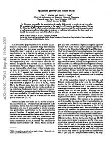
FIG. 1: The correction function (27) as a function of the scale factor (solid line). The asymptotic form (28) for large a is shown by the dashed line. (The sharp cusp, a consequence of the absolute value appearing in (27), is present only for eigenvalues as plotted here, but would disappear for expectation values of the inverse volume operator in coherent states. This cusp will play no role in the analysis of this paper.)

− 21 adα/da with the scale factor a related to q by q = det(qab ) = a6 . In this case the quantum gravitational expectation for α(q), as per Eqs. (A9) and (A10), simplifies. To use these expressions, we have to relate the scale factor to quantum gravitational excitation levels as they occur in calculations of loop quantum gravity. In the notation of the appendix, an elementary discrete patch in a nearly isotropic space-time has, on the one hand, an area of ℓ20 a2 if ℓ0 is the coordinate diameter of the patch. This can be expressed as ℓ20 a2 = (VV /NV )2/3 where NV is the number of patches in a box V of volume VV . On the other hand, using (A2) the quantum gravity state assigns a value of 4πγℓ2Pµv to this patch via the flux operator, where µv is the quantum number of the geometrical excitation of this patch. Thus, we obtain 2/3

µv =

VV

2/3

4πγℓ2P NV

=:

a2 a2disc

NV V0

1/3

where adisc

√ = 2 πγℓP



(26)

with the coordinate volume V0 of the box V. The numerical value of adisc depends on coordinates via V0 , or on the normalization of the scale factor. (It does not depend on the choice of the box V because a change would multiply NV and V0 by the same factor.) But it is important to note that adisc is not just determined by the Planck length ℓP , which appears for dimensional reasons, but also depends on the large number NV of discrete patches per volume as given by the quantum gravity state. This is exactly a parameter as expected in the discussion of Sec. II. Replacing µv in the equations of the appendix, we obtain 2  √ α(a) = 8 2(a/adisc )2 (2(a/adisc)2 + 1)1/4 − |2(a/adisc )2 − 1|1/4

(27)

where adisc appears, influencing the size of quantum gravity corrections. √ The function is plotted in Fig. 1. One can easily see √ that α(a) approaches the classical value−1α = 1 for a ≫ adisc / 2, while it differs from one for small a. For a > adisc / 2, the corrections are perturbative in a , α(a) ∼ 1 +

7  adisc 4 + ··· . 64 a

(28)

9 This is the first correction in an asymptotic expansion for eigenvalues. If semiclassical states rather than volume eigenstates are used, powers of a−1 in the leading corrections can be smaller. Moreover, via NV the discreteness scale adisc is expected to be not precisely constant but a function of a itself because the underlying spatial discreteness of quantum gravity can be refined dynamically during cosmological evolution [23, 24]. (Indeed, dynamical refinement is also required for several other phenomenological reasons [25, 26, 27, 28, 29].) In our following analysis we will thus assume a functional form α(a) = 1 + c(a/a0 )−n

(29)

where we traded the fundamental normalization by adisc for normalization with respect to the present-day value of the scale factor a0 . From the derivation, n is likely to be a small, even integer and c is known to be positive. The constant c depends on adisc and inherits the NV -factor. It can thus be larger than of order one. We will treat this parameter as phenomenological and in the end formulate bounds on c as bounds for NV . Energy density and the pressure then are, ignoring the classical interaction term B, ρeff = and 3Peff =




2Eia α(a) −βDa πξT τ i ξ + πχT τ i χ + i −θL πξT τ i Da ξ − θR πχT τ i Da χ − c.c. 6 a

 


d log α 2Eia −βDa πξT τ i ξ + πχT τ i χ + i −θL πξT τ i Da ξ − θR πχT τ i Da χ − c.c. . α(a) 1 − 6 a d log a

From this, the equation of state w can easily be computed:   d log α 1 1− . weff = 3 d log a

(30)

(31)

(32)

This quantum gravity correction is independent of the specific matter dynamics as in the classical relativistic case. It results in an equation of state which is linear in ρ, but depends on the geometrical scales (and the Planck length) through α. This is the same general formula derived in [6] for radiation. Thus, on an isotropic background radiation and relativistic fermions are not distinguished by the form of quantum corrections they receive. With the equation of state and the continuity equation a˙ ρ˙ + 3 (ρ + P ) = 0 , a

(33)

where a is the scale factor and the dot indicates a proper time derivative, we can determine energy density as a function of the universe size. We first obtain d log ρ(a) = −3 (1 + w(a)) , d log a explicitly showing the dependence of the equation of state on the scale factor. The solution is  Z  ρ(a) = ρ0 exp −3 (1 + w(a)) d log a ,

(34)

(35)

where ρ0 is the integration constant. Inserting an equation of state of the form (32) we obtain ρ(a) = ρ0 α(a)a−4 .

(36)

For α = 1, we retrieve the classical result ρ(a) ∝ a−4 , but for α 6= 1 loop quantum gravity corrections induced by the discreteness of flux operators are reflected in the evolution of energy density in a Friedmann–Robertson–Walker universe. V.

EFFECT ON BIG BANG NUCLEOSYNTHESIS

The production of elements in the early universe is highly sensitive to the expansion rate, given by  1/2 a˙ 8 = πGρ , a 3

(37)

10 where ρ is the total density, thus including radiation and fermions. As we have seen here for fermions and in [6] for radiation, the effect of loop quantum gravity corrections is to multiply the effective ρ(a) by a factor α(a). Most importantly, we find that α(a) is the same for both bosons and fermions (up to possible quantization ambiguities), so a separate treatment of the two types of particles in the early universe (as in Ref. [1]) is unnecessary here. In the standard treatment of the thermal history of the universe, the density of relativistic particles (bosons or fermions) is given by ρ=

π2 g∗ T 4 , 30

(38)

where g∗ is the number of spin degrees of freedom for bosons, and 7/8 times the number of spin degrees of freedom for fermions, and T is the temperature, which scales as T ∝ a−1 .

(39)

w = 1/3.

(40)

The equation of state parameter is

Clearly, equations (38)–(40) are inconsistent with equations (32) and (36). There is some ambiguity in determining the correct way to modify the expressions for ρ(T ) and w. We have chosen to assume that the modifications are contained in the gravitational sector, so that the density is given by ρ = α(a)

π2 g∗ T 4 , 30

(41)

with the temperature scaling as in equation (39), and the equation of state w is given by equation (32). This guarantees that the standard continuity equation (33) continues to hold. Note that this is not the only way to incorporate equation (36) into the calculation, but it seems to us the most reasonable way. This issue requires a consideration of thermodynamics on a quantum space-time, which is a fascinating but not well-studied area. Instead of entering details here, we note that we interpret the α-correction as a consequence of a quantum gravity sink to energy and entropy. Thus, quantum gravity implies a non-equilibrium situation which would otherwise imply that ρ must be proportional to T 4 without any additional dependence on a ∝ T −1 . With these assumptions, we can simply treat α(a) as an effective multiplicative change in the overall value of G. Note that this simplification is only possible because we explicitly derived by our canonical analysis that, unexpectedly, quantum corrections of radiation and fermions appear in similar forms. This makes possible a comprehensive derivation of implications for BBN, bearing on earlier work. In fact, a great deal of work has been done on the use of BBN to constrain changes in G (see, e.g. Refs. [30, 31, 32, 33, 34]). The calculation is straightforward, if one has a functional form for the time-variation in G. For the loop quantum gravity corrections considered here, the most reasonable functional form is (29). Note that this expression is by construction valid only in the limit where α(a) − 1 ˙ and the neutron-to-proton ratio ∼ 1 MeV, the weak-interaction rates are faster than the expansion rate, a/a, (n/p) tracks its equilibrium value exp[−∆m/T ], where ∆m is the neutron-proton mass difference. As the universe expands and cools, the expansion rate becomes too fast for weak interactions to maintain weak equilibrium and n/p freezes out. Nearly all the neutrons which survive this freeze-out are converted into 4 He as soon as deuterium becomes stable against photodisintegration, but trace amounts of other elements are produced, particularly deuterium and 7 Li (see, e.g., Ref. [35] for a review). In the standard model, the predicted abundances of all of these light elements are a function of the baryon-photon ratio, η, but any change in G alters these predictions. Prior to the era of precision CMB observations (i.e., before

11 WMAP), Big Bang nucleosynthesis provided the most stringent constraints on η, and modifications to the standard model could be ruled out only if no value of η gave predictions for the light element abundances consistent with the observations. However, the CMB observations now provide an independent estimate for η, which can be used as an input parameter for Big-Bang nucleosynthesis calculations. Copi et al. [33] have recently argued that the most reliable constraints on changes in G can be derived by using the WMAP values for η in conjuction with deuterium observations. The reason is that deuterium can be observed in (presumably unprocessed) high-redshift quasi stellar object (QSO) absorption line systems (see Ref. [36] and references therein), while the estimated primordial 4 He abundance, derived from observations of low metallicity HII regions, is more uncertain (see, for example, the discussion in Ref. [37]). While we agree with the argument of Copi et al. in principle, for the particular model under consideration here it makes more sense to use limits on 4 He than on deuterium, in conjunction with the WMAP value for η. The reason is that the 4 He abundance is most sensitive to changes in the expansion rate at T ∼ 1 MeV, when the freeze-out of the weak interactions determines the fraction of neutrons that will eventually be incorporated into 4 He. Deuterium, in contrast, is produced in Big Bang nucleosynthesis only because the expansion of the universe prevents all of the deuterium from being fused into heavier elements. Thus, the deuterium abundance is most sensitive to the expansion rate at the epoch when this fusion process operates (T ∼ 0.1 MeV). The importance of this distinction with regard to modifications of the standard model was first noted in Ref. [38], and a very nice quantitative analysis was given recently in Ref. [39]. Note that our estimate for the behavior of G(a)/G0 − 1, equation (42), is a steeply decreasing function of a. Thus, the change in the primordial 4 He abundance will always be much larger than the change in the deuterium abundance. Therefore, we can obtain better constraints on this model by using extremely conservative limits on 4 He, rather than by using the more reliable limits on the deuterium abundance. For the same reason, we can ignore any effect on the CMB, since the latter is generated at a much larger value of a, and any change will be minuscule. Hence, we can confidently use the WMAP value for η. WMAP gives [40] −10 η = 6.116+0.197 . −0.249 × 10

(44)

Because the estimated errors on η are so small, we simply use the central value for η; the bounds we derive on c in equation (29) change only slightly when η is varied within the range given by equation (44). Since c in equations (29) and (42) is thought to be positive, the effect of LQG corrections is to increase the primordial expansion rate, which increases the predicted 4 He abundance. We therefore require an observational upper bound on the primordial 4 He abundance. As noted earlier, this is a matter of some controversy. We therefore adopt the very conservative upper bound recommended by Olive and Skillman [37]: YP ≤ 0.258,

(45)

α = 1+e c/an10

(46)

where YP is the primordial mass fraction of 4 He. For a fixed value of n in equation (42), we determine the largest value of c that yields a primordial 4 He abundance consistent with this upper limit on YP . Since we are essentially bounding the change in G at a/a0 ∼ 10−10 , it is convenient to rewrite equation (29) as 10

where a10 ≡ 10 (a/a0 ). This upper bound on e c as a function of n is given in Fig. 2. For the special case n = 4, we can use these results to place a bound on adisc in equation (28). We obtain adisc < 2.4 × 10−10 . (47) a0 This is not a strong bound for the parameters of quantum gravity, but clearly demonstrates that quantum corrections are consistent with successful big bang nucleosynthesis. In terms of more tangible quantum gravity parameters, we have 1/3

NV

1/3


1 one can directly check that corrections are positive, i.e. αv,K > 1 in this regime. Expressing the labels in terms of the densitized triad through fluxes (A2) results in functionals α[pI (v)] = αv,K (4πγℓ2P µv,I )

(A11)

which enter quantum corrections.

[1] [2] [3] [4] [5] [6] [7]

J. Barrow and R. J. Scherrer, Phys. Rev. D 70, 103515 (2004), [astro-ph/0406088]. M. Bojowald, Living Rev. Relativity 8, 11 (2005), [gr-qc/0601085], http://relativity.livingreviews.org/Articles/lrr-2005-11/. C. Rovelli, Cambridge University Press, Cambridge, UK, 2004. A. Ashtekar and J. Lewandowski, Class. Quantum Grav. 21, R53–R152 (2004), [gr-qc/0404018]. T. Thiemann, Introduction to Modern Canonical Quantum General Relativity, [gr-qc/0110034]. M. Bojowald and R. Das, Phys. Rev. D 75, 123521 (2007). M. Bojowald, H. Hern´ andez, M. Kagan, P. Singh, and A. Skirzewski, Phys. Rev. Lett. 98, 031301 (2007), [astro-ph/0611685]. [8] M. Bojowald, AIP Conf. Proc. 917, 130–137 (2007), [gr-qc/0701142]. [9] F. W. Hehl, P. von der Heyde, G. D. Kerlick and J. M. Nester, Rev. Mod. Phys. 48, 393–416 (1976). [10] J. F. Barbero G., Phys. Rev. D 51, 5507–5510 (1995), [gr-qc/9410014].

15 [11] [12] [13] [14] [15] [16] [17] [18] [19] [20] [21] [22] [23] [24] [25] [26] [27] [28] [29] [30] [31] [32] [33] [34] [35] [36] [37] [38] [39] [40] [41] [42] [43] [44] [45] [46]

G. Immirzi, Class. Quantum Grav. 14, L177–L181 (1997). S. Holst, action, Phys. Rev. D 53, 5966–5969 (1996), [gr-qc/9511026]. A. Ashtekar, Phys. Rev. D 36, 1587–1602 (1987). A. Perez and C. Rovelli, Phys. Rev. D 73, 044013 (2006), [gr-qc/0505081]. L. Freidel, D. Minic, and T. Takeuchi, Phys. Rev. D 72, 104002 (2005), [hep-th/0507253]. S. Mercuri, Phys. Rev. D 73, 084016 (2006), [gr-qc/0601013]. M. Bojowald and R. Das, Canonical Gravity with Fermions, arXiv:0710.5722. T. Thiemann, Class. Quantum Grav. 15, 1487–1512 (1998), [gr-qc/9705021]. T. Thiemann, Class. Quantum Grav. 15, 1281–1314 (1998), [gr-qc/9705019]. M. Bojowald and A. Skirzewski, Rev. Math. Phys. 18, 713–745 (2006), [math-ph/0511043]. M. Bojowald and A. Skirzewski, Int. J. Geom. Math. Mod. Phys. 4, 25–52 (2007), [hep-th/0606232]. M. Bojowald, H. Hern´ andez, M. Kagan, and A. Skirzewski, Phys. Rev. D 75, 064022 (2007), [gr-qc/0611112]. M. Bojowald, Gen. Rel. Grav. 38, 1771–1795 (2006), [gr-qc/0609034]. M. Bojowald, Gen. Rel. Grav. 40, 639–660 (2008), [arXiv:0705.4398] A. Ashtekar, T. Pawlowski and P. Singh, Phys. Rev. D 74, 084003 (2006), [gr-qc/0607039]. M. Bojowald, D. Cartin and G. Khanna, Phys. Rev. D 76, 064018 (2007), [arXiv:0704.1137]. W. Nelson and M. Sakellariadou, Phys. Rev. D 76, 044015 (2007), [arXiv:0706.0179]. W. Nelson and M. Sakellariadou, Phys. Rev. D 76, 104003 (2007), [arXiv:0707.0588]. M. Bojowald and G. M. Hossain, Phys. Rev. D 77, 023508 (2007), [arXiv:0709.2365]. J.D. Barrow, Mon. Not. R. Astr. Soc. 184, 677 (1978). J. Yang, D.N. Schramm, G. Steigman, and R.T. Rood, Astrophys. J. 227, 697 (1979). F.S. Accetta, L.M. Krauss, and P. Romanelli, Phys. Lett. B 248, 146 (1990). C.J. Copi, A.N. Davis, and L.M. Krauss, Phys. Rev. Lett. 92 (2004) 171301. T. Clifton, J.D. Barrow, and R.J. Scherrer, Phys. Rev. D 71 (2005) 123526. K.A. Olive, G. Steigman, and T.P. Walker, Phys. Rep. 333 (2000) 389. D. Kirkman, D. Tytler, N. Suzuki, J.M. O’Meara, and D. Lubin, Ap.J. Suppl. 149 (2003) 1. K.A. Olive and E.D. Skillman, Ap.J, 617 (2004) 29. E.W. Kolb and R.J. Scherrer, Phys. Rev. D 25 (1982) 1481. C. Bambi, M Giannotti, and F.L. Villante, Phys. Rev. D 71 (2005) 123524. D.N Spergel, et al., astro-ph/0603449. M. Bojowald, Class. Quantum Grav. 19, 5113–5130 (2002), [gr-qc/0206053]. M. Bojowald, Pramana 63, 765–776 (2004), [gr-qc/0402053]. M. Bojowald, Class. Quantum Grav. 17, 1489–1508 (2000), [gr-qc/9910103]. M. Bojowald, Class. Quantum Grav. 21, 3733–3753 (2004), [gr-qc/0407017]. T. Thiemann, Class. Quantum Grav. 15, 839–873 (1998), [gr-qc/9606089]. We are not assuming strict isotropy to compute quantum corrections of inhomogeneous fermion fields. Nevertheless, in leading order corrections one can use the background geometry.