Abstract. Rotating modulation collimator (RMC) is an important imaging technique in hard X-ray astronomy. With traditional inversion techniques, the sensitivity, ...
SUPPLEMENT SERIES
Astron. Astrophys. Suppl. Ser. 128, 363-368 (1998)
Direct demodulation technique for rotating modulation collimator imaging Y. Chen, T.P. Li, and M. Wu
High Energy Astrophysics Lab, Institute of High Energy Physics, Chinese Academy of Sciences, Beijing, China Received June 21, 1996 accepted June 4, 1997
Abstract. Rotating modulation collimator (RMC) is an Sood et al. 1996) for hard X-ray imaging. Nishimura et al. important imaging technique in hard X-ray astronomy. With traditional inversion techniques, the sensitivity, angular resolution and ability of simultaneous imaging of point sources and extended emission are not good enough in many practical cases. In this work, a new inversion technique, the direct demodulation method, is applied to analyse simulated data of an RMC telescope. The results show that the image quality from direct demodulation are improved signi�cantly in comparison with that from traditional inversion techniques, such as the cross-correlation method and the CLEAN cross-correlation method. From an RMC telescope with a simple bi-grid collimator and the direct demodulation technique, we can do imaging for both discrete and extended sources.
(1978) used a balloon-borne wide-�eld RMC instrument to localise gamma-ray bursts. In the mid-1970s, three satellites equipped with RMC systems, Ariel 5, SAS-3 and Hakucho, were launched. The hard X-ray RMC telescope WATCH is currently operating on the GRANAT satellite (Lund 1985).
Key words: X-rays: general | methods: data analysis 1. Introduction
Imaging is a di cult task in hard X-ray and soft -ray astronomy. For soft X-rays (10 MeV), multilayer spark chambers can be used, in which the direction of an incident photon may be determined from the electron-positron pair that it creates. But in hard X-ray and soft -ray range (from tens keV to several MeV), these techniques are no longer useful. Imaging can be achieved only by applying aperture modulation techniques. The scanning modulation collimator with two grids was �rst put forward by Oda (1965) for imaging X-ray sources without focusing and without a position sensitive detector. Shortly after, it was suggested that a rotating collimator may be better (Mertz 1968). The RMC was �rst proposed for X-ray astronomy by Schnopper et al. (1968). The RMC technique was successfully used in a number of rocket ights (Schnopper et al. 1970� Cruise & Willmore 1975) and balloon-borne experiments (Staubert et al. 1983� Ubertini et al. 1985�
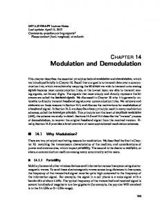
Fig. 1.
Rotating modulation collimators
Figure 1 illustrates a typical structure of RMC. Two identical and parallel wire grids with absorbing and transmitting strips of equal width a are rotated about their axis. The transmission ratio of photon ux from a source will change with the rotation angle �, which results in a temporal-modulated intensity of the photon ux transmitted to the detector. For a point source with coordinates (r� �0 ) and intensity I0 , the intensity received by the detector is I(�) = I0 p(�� r)
(1)
2. Methods of inversion
In observations with any kind of telescope, the relation between the observational data d(k) and the intensity distribution f(i) of a sky region can be described by the following observation equation system (modulation equation system):
Xn p(k� i)f(i) = d(k) i=1
(k = 1� :::� m)
(4)
where the modulation coe cient of the telescope, p(k� i), is the contribution of a unit intensity source placed at the Fig. 2. A typical modulation signature of RMC, which is the sky bin i to the kth observed data, which represents the expected observed intensity I against rotating angle � for a instrument response character. The equation system (4) can be written in matrix form as point source with unit intensity where p(�� r) is the modulation function of RMC p(�� r) = 2" j 1 ; r cos(� ; �0 )=a + �r cos(� ; �0 )=a] j (2) where " is the detection e ciency, �x] the integer which satis�es �x] � x < �x + 1] and 0 � � < �. There exists a \ghost" image at �0 + � which can be removed by a certain o�set between the grids in the two planes. The intrinsic angular resolution of the RMC system is �0 = arctan Ha : (3) A typical modulation signature of RMC is shown in Fig. 2. Compared with other techniques, e.g. coded aperture masks, RMC has a larger �eld of view and does not require a position-sensitive detector. RMC can be constructed in simple and cost-e�ective structure, which makes it attractive, particularly in wide-�eld monitoring. Since the raw data of RMC is a modulated count rate varying with time, it needs a suitable inversion treatment for the observed data to reconstruct an image of the X-ray sky. The traditional technique to determine the source position is Fourier analysis of the intensity or crosscorrelation analysis of the observed intensity function with the modulation function. Images from a traditional inversion technique usually have complicated sidelobes. Their sensitivity and angular resolution are not good enough in many practical cases. Imaging for extended sources is still a di cult problem for the RMC technique. The direct demodulation method (DDM) has been put forward in the early 1990s and proved to be e�ective in many inversion cases in high-energy astrophysics (Li & Wu 1992, 1993, 1994). We have made a simulation study to apply this technique to analyse RMC data and have gotten results showing signi�cant improvement in the qualities of RMC images. We give a brief description of the direct demodulation method in Sect. 2. The results of applying the direct demodulation technique to analyse simulated RMC data are presented in Sect. 3 and brief discussions in Sect. 4. Int
Int
Int
Int
P f = d:
(5)
In space high-energy astronomy, the cross-correlation technique is now widely used to reconstruct the object f from the observed data d, i.e. to take the cross-correlation distribution c of the data and the modulation function as a reconstruction of object intensity f � c = P Td:
(6)
The angular resolution of a cross-correlation map �cc is approximately equal to the intrinsic resolution �0 of the instrument, i.e. �cc ' �0 . The cross-correlation distribution is not a satisfactory reconstruction of the object in RMC imaging. The results from CCM usually have sidelobes. Therefore, faint sources are often covered by sidelobes of strong sources. To solve this problem, the CLEAN technique (Hogbom 1974) can be used in the cross-correlation. In this technique, some fraction of ux of bright point sources is subtracted from a cross-correlation image, and more faint sources can be detected. This process continues until a certain closure criterion is satis�ed. We may call it CLEAN cross-correlation. Multiplying the two sides of Eq. (5) by the transpose, P T, of the modulation matrix, we derive the following correlation equation system P f =c
(7)
0
where c = P Td� P = P TP . From Eq. (7), one can see that c 6= f, the relation between c and f being described by the correlation Eq. (7). The cross-correlation c is just an image of the object f through a modulation (distortion) of a certain imagery instrument with a point-spread function (PSF) P = P T P. The cross-correlation technique simply uses c instead of f, completely ignoring the information included in Eq. (7) about the observation, which is the main reason of unsatisfactory image quality derived by cross-correlation deconvolution. 0
0
Fig. 3. Images from the simulated data of a single point source observed by a RMC system with height H = 95 cm, strip width a = 1:0 cm and FOV=6o 6o . a) Object. b) Cross-correlation map. c) CLEAN cross-correlation map. d) Image from direct
demodulation
The direct demodulation technique performs a further deconvolution from c by solving Eq. (7) iteratively under proper physical constraints (Li & Wu 1992, 1993, 1994). The calculation formula of the direct demodulation algorithm by using Gauss-Seidel iterations is (8) fi(l+1) = p1 (ci ; pij fj(l) ) ii j =i
X
data d to get background data db , calculate cb = P T db and then iteratively solve the following correlation equation P b = cb 0
(10)
with a smooth procedure or under a continual constraint (for details see Li & Wu 1994) to get b. The stability, convergency and global optimum property of the Li-Wu with the constraint condition algorithm of direct demodulation have been proved by the fi � bi (9) theory of neural computing (Li 1997). where the lower intensity limit bi is the background inten- 3. Simulations sity. In the case of no priori knowledge of the di�use background, the intensity lower limit b can be estimated from We made computer simulations to compare the quality the data: Use a successive procedure to subtract the con- of images from direct demodulation with that from crosstribution of apparent discrete sources from the observed correlation deconvolution and other methods for the same 0
6
0
Fig. 4. Discriminating two nearby sources. a) Object scene. b) Cross-correlation d) Image from direct demodulation. e) Image from Richardson-Lucy iterations
map. c) CLEAN cross-correlation map.
simulated RMC data. The following normalized cross- two neighbouring bins should not be greater than a certain value. correlation function was used in our calculations c(i) =
X(pki ; pi)dk= X(pki ; pi) : 2
k
k
vuuXm m X s(i) = c(i) p(k� i)=t d(k)
(11)
To estimate the background, we calculated k=1
k=1
(i = 1� :::� n)
(12)
then found the bin with maximum s(i) and subtracted the contribution of the apparent discrete source at point i from the data. The background data db was obtained by repeating the above procedure until the maximumvalue of s(i) was less than a given threshold. The background b can be found by solving Eq. (10) iteratively. In the iterations, a continual constraint was used, i.e. the di�erence between
3.1. Imaging for point sources
In the simulations, we used an RMC telescope structured as in Fig. 1 with strip width a = 1:0 cm, the separation of the two grids H = 95 cm, the total active area of the detector 1000 cm2 and FOV= 6o � 6o . To avoid \ghost" peaks in the image, we set up a 0.5 cm o�set between the grids in the two planes. The background is assumed to be 0.09 counts cm 2 s 1 and the observation time is 24 hours. We �rst supposed that only a single point source exists in the FOV at the position (;0: 050� 1: 350) (see Fig. 3a) with a ux of 1 10 2 ph cm 2 s 1. The rotating period was divided into 400 units (m = 400). A Monte Carlo sample of observed data of the RMC telescope was produced. The cross-correlation map and ;
;
�
;
;
�
;
CLEAN cross-correlation map from the simulated data are shown in Figs. 3b and c respectively. For the same simulated data, we did image analysis by the direct demodulation method and got the result shown in Fig. 3d. From the direct demodulation map, we �nd the position of the point source at (;0: 060 0: 002� 1: 353 0: 003) and ux (1:00 0:02) 10 2 ph cm 2 s 1, which is consistent with the assumed values. The errors of the position and counts are the standard deviations of values of the quantities measured for images from twenty Monte Carlo samples. It is clear from comparing Fig. 3d with Fig. 3b that the direct demodulation technique can signi�cantly improve the angular resolution. The FWHM of the point-source image in Fig. 3d from DDM is 0: 2, much smaller than that in Fig. 3b from CCM, 0: 5. The cross-correlation maps, Fig. 3b and c, show severe sidelobes around the image of the point source. The image derived by using the direct demodulation technique with the same simulated data, Fig. 3d, has a much clearer background. For further comparing the angular resolution ability of the two methods, we set up two point sources placed at (;0: 050� 1: 350) and (;0: 550� 1: 350) with uxes 2 10 2 ph cm 2 s 1 and 1 10 2 ph cm 2 s 1 , respectively. The results of image analyses by CCM, CLEAN CCM and DDM are shown in Figs. 4b, c and d, respectively. From Fig. 4d, one can see that the direct demodulation technique can clearly discriminate the two point sources with a separation smaller than the intrinsic resolution of the telescope, while the cross-correlation and the CLEAN cross-correlation cannot. Figure 4d gives two point sources sited at (;0: 070 0: 006� 1: 38 0: 02) and (;0: 48 0: 03� 1: 32 0: 03) with uxes 1:8 10 2 ph cm 2 s 1 and 8:9 10 3 ph cm 2 s 1 , respectively. We also tried the Richardson-Lucy algorithm (Richardson 1972� Lucy 1974) and got an image shown in Fig. 4e, in which many false sources appear and from which the uxes of the two sources are 4:5 10 3 ph cm 2 s 1 and 1:8 10 3 ph cm 2 s 1 , much less than the assumed values. �
�
;
;
�
�
;
�
�
�
;
�
;
�
;
�
�
�
;
�
;
�
;
�
�
�
�
;
;
;
;
;
;
;
;
;
;
;
;
3.2. Imaging for both point and extended sources
It is di cult to give correct source locations and intensities in the case of multi-source imaging with a single RMC and the cross-correlation deconvolution. Simultaneous imaging for both point and extended sources is also di cult by a single RMC. Figure 5a shows an object scene with two point sources and an extended source. The uxes of the two point sources are assumed to be 2 10 2 and 5 10 3 ph cm 2 s 1 , respectively, and the total ux of the extended source 3:6 10 2 ph cm 2 s 1 . The background, the observational duration and the RMC system con�guration are assumed to be the same as that in subsection 3.1. Figure 5b shows the cross-correlation map from the simulated data and Fig. 5c the CLEAN cross-correlation ;
Imaging for point and extended sources by a single RMC with strip width a = 1:0 cm, height H = 95 cm and FOV=6o 6o . a) The object scene. b) Cross-correlation deconvolution. c) CLEAN cross-correlation. d) Direct demodulation reconstruction
Fig. 5.
;
;
;
;
;
;
map, from which only the strong point source can be identi�ed. For the same simulated data, we made a direct demodulation reconstruction and got the result shown in Fig. 5d. Besides the strong point source, an image of the weak point source and structure of the extended source can also be seen from Fig. 5d. The uxes estimated from Fig. 5d are 2:0 10 2 and 5:7 10 3 ph cm 2 s 1 for the two point sources and 2:9 10 2 ph cm 2 s 1 for the extended source, respectively. ;
;
;
;
;
;
;
4. Discussion
In this paper, we apply the direct demodulation technique to analyse simulated data of a rotating modulation collimator telescope for the �rst time. The direct demodulation method has already been applied successfully to image analysis for various kinds of data in high energy-astronomy, e.g. for data of -ray imaging telescope COS-B (Li & Wu 1990), for scan observation data of slat collimator telescopes: the scan imaging for CygX1 by the balloon-borne hard X-ray collimated telescope HAPI-4 (Lu et al. 1995) and for EXOSAT-ME data of the galactic plane survey (Lu et al. 1996), for data from the Compton scatter telescope COMPTEL/CGRO (Zhang et al. 1996). Simulation results show that the direct demodulation technique can signi�cantly improve imaging quality of the coded mask aperture telescope (Li 1995). As seen in this paper, the application of this method to telescopes based on a rotating modulation collimator is also feasible. Images from RMC with the direct demodulation technique have much higher angular resolution than those with cross-correlation analysis. The direct demodulation images have almost no sidelobes and can represent both discrete and extended structures. After considering the improved performance with the direct demodulation method, the RMC technique might be more competitive for future imaging instrumentation in high-energy astronomy. Acknowledgements. The authors thank Dr. F.J. Lu and Y.X. Feng for helpful discussions. This work was supported by the National Natural Science Foundation of China.
References
Cruise A., Willmore A., 1975, MNRAS 170, 165 H�ogbom J., 1974, A&AS 15, 417 Li T.P., 1995, Exper. Astron. 6, 63 Li T.P., 1997, Space observation of hard X-rays, in: Hu W.R. (eds.) Space Science in China. Gordon & Breach Science Publishers Li T.P., Wu M., 1990, Acta Astron. Sinica 31, 393 Li T.P., Wu M., 1992, A direct method for spectral and image restoration, in: Astronomical Data Analysis Software and System I., Worrall D.M., Biemesderter C. & Barnes J. (eds.) A.S.P. Conf. Ser. 25, 229 Li T.P., Wu M., 1993, Ap&SS 206, 91 Li T.P., Wu M., 1994, Ap&SS 215, 213 Lu F.J., Li T.P., Sun X.J., Wu M., Page C.G., 1996, A&AS 115, 395 Lu Z.G., Wang J.Z., Li Y.G., et al., 1995, Nucl. Instr. Meth. Phys. Res. Sec. A 362, 551 Lucy L.B., 1974, AJ 79, 745 Lund N., 1985, SPIE Symp. 597, 95 Mertz L., 1968, Proc. Symp. Mod. Opt. 17, 787 Nishimura J., Fuji M., et al., 1978, Nat 272, 337 Oda M., 1965, Appl. Opt. 4, 143 Richardson B.M., 1972, J. Opt. Soc. Am. 62, 55 Schnopper H.W., Thompson R.I., Watt S., 1968, Space Sci. Rev. 8, 534 Schnopper H.W., et al., 1970, ApJ 161, L161 Sood R.K., Panettieri J., Grey D., Woods G., Ho�mann J., Manchanda R.K., Staubert R., Kendziorra E., Rochester G.K., 1996, Pub. Astr. Soc. Austr. 13, 156 Staubert R., Theinhardt J., Kendziorra E., 1983, Proc. 18th Int. Cosmic Ray Conf. 9, 347 Ubertini P., Barbanera L., Bazzano A., et al., 1985, Proc. 2nd Int. Symp. on Optical and Electro-Optical Science, SPIE Vol. 597, p. 74 Zhang S., Li T.P., Wu M., Yu W.F., Song L.M., Lu F.J., Feng Y.X., 1997, in Proc. of 4th Compton Symp., Williamsburg AIP Conf. Proc., Dermer C.D. & Kurfess J.D. (eds.)