direct detection with vector mediators - arXiv

SCIPP 16/07

arXiv:1605.04917v1 [hep-ph] 16 May 2016

You can hide but you have to run: direct detection with vector mediators Francesco D’Eramo a,b , Bradley J. Kavanagh c,d , Paolo Panci e a

Department of Physics, University of California Santa Cruz, 1156 High St., Santa Cruz, CA 95064, USA b

Santa Cruz Institute for Particle Physics, 1156 High St., Santa Cruz, CA 95064, USA c

Laboratoire de Physique Théorique et Hautes Energies, CNRS, UMR 7589, 4 Place Jussieu, F-75252, Paris, France d

e

Institut de Physique Théorique, Université Paris Saclay, CNRS, CEA, F-91191 Gif-sur-Yvette, France

Institut d’Astrophysique de Paris, UMR 7095 CNRS, Université Pierre et Marie Curie, 98 bis Boulevard Arago, Paris 75014, France

Abstract We study direct detection in simplified models of Dark Matter (DM) in which interactions with Standard Model (SM) fermions are mediated by a heavy vector boson. We consider fully general, gauge-invariant couplings between the SM, the mediator and both scalar and fermion DM. We account for the evolution of the couplings between the energy scale of the mediator mass and the nuclear energy scale. This running arises from virtual effects of SM particles and its inclusion is not optional. We compare bounds on the mediator mass from direct detection experiments with and without accounting for the running and find that in some cases these bounds differ by several orders of magnitude. We also highlight the importance of these effects when translating LHC limits on the mediator mass into bounds on the direct detection cross section. For an axial-vector mediator, the running can alter the derived bounds on the spin-dependent DM-nucleon cross section by a factor of two or more. Finally, we provide tools to facilitate the inclusion of these effects in future studies: general approximate expressions for the low energy couplings and a public code runDM to evolve the couplings between arbitrary energy scales.

1

Contents 1 Introduction

2

2 Simplified Models for Vector Mediators

3

3 Low-energy couplings and direct detection rates

6

4 Direct detection bounds on benchmark models 4.1 Benchmark I: flavor universal couplings to quarks . . . . . . . . . . . . . . . . . 4.2 Benchmark II: flavor universal couplings to leptons . . . . . . . . . . . . . . . . 4.3 Benchmark III: couplings to third generation . . . . . . . . . . . . . . . . . . . .

9 10 14 17

5 Rescaling and general limits

21

6 Connecting direct detection and collider searches

22

7 Conclusions

24

A A simple analytical solution for the RGE

25

B runDM: a code for the RGE

29

C Details of the matching at the nuclear scale

32

D Projected LZ limits

35

1

Introduction

Astrophysical and cosmological observations over the last four decades have accumulated indisputable evidence for dark matter (DM) [1]. This important component of our universe, five times more abundant than baryonic matter, cannot be accounted for by any Standard Model (SM) degree of freedom. The question of the origin and composition of DM is hence among the most urgent in particle physics [2]. A stable Weakly Interacting Massive Particle (WIMP) with weak-scale mass and cross section provides a compelling solution. WIMPs naturally appear in well-motivated beyond the SM frameworks [3–7]. Interactions with SM fields, responsible in the early universe for relic DM production through thermal freeze-out [8–10], today allow different and complementary experimental search strategies. Crucially, each search strategy probes DM interactions at different energy scales. In order to properly explore complementarity, one must carefully make the connection between physics at high and low energy. Such a scale connection is achieved by employing techniques from Effective Field Theory (EFT), performing a Renormalization Group (RG) analysis of DM interactions. This RG Evolution (RGE) typically introduces mixing between different DM-SM interactions, affecting the size of couplings, or even inducing new couplings which do not appear in a na¨ıve comparison [11–23]. These effects do not depend on the properties of the Dark Sector and are not optional; they arise solely from RGE of the couplings via SM loops.

2

Our focus here is on direct detection (DD) experiments [24, 25], which search for O(∼ keV) low energy DM-nucleon recoils, meaning that the separation of scales can be large compared with high energy probes such as the Large Hadron Collider (LHC). DD experiments also involve matrix elements which are extremely sensitive to the Lorentz structure of the effective operator under consideration [24], meaning that operator mixing can have a substantial impact. This work analyzes theories of DM where interactions with SM fermions are mediated by a massive vector boson. At energies below the mediator mass, DM-SM couplings are described by higher-dimensional contact interactions between spin-1 currents, similarly to the low-energy theory for SM weak interactions. The scale connection in this class of models can be performed by solving the RG equations derived in Ref. [21]. Although the authors of Ref. [21] only considered fermionic DM χ interacting through the vector current χγ µ χ, the RGE is driven by the SM current part of the contact interactions, and thus their RG equations are valid for other DM spins and interaction structures. We expand and generalize that work in two key ways. First, we consider a wider range of DM spins and interaction structures, constructing the most general model for SM fermions interacting with scalar or fermion DM through the exchange of a vector mediator. Second, we do not limit the analysis to standard spin-dependent (SD) and spin-independent (SI) DM-nucleon interactions. We also consider higher-order non-relativistic DM-nucleon interactions [26], which in some cases give rise to limits where none are expected in the standard SI/SD framework. We present the results of our study as follows. In Sec. 2, we introduce the simplified model framework for vector mediators, coupling the mediator to SM fermions without breaking SM electroweak gauge invariance. DD rates are computed by following the general procedure outlined in Sec. 3. The key results of this paper are then summarized in Figures 1 to 6 of Sec. 4, where we give DD limits on the mass of the mediator for three different sets of benchmark couplings. We quantify the size of the RGE effects by presenting our results both with and without accounting for them. These limits can be easily generalized to any choice of couplings by following the prescription given in Sec. 5. Complementarity with LHC bounds is explored in Sec. 6; Figure 7 shows an example of how limits on simplified models from the LHC can be translated into the (mχ , σχN ) plane of direct detection and how the RGE affects this translation. Finally, our conclusions are given in Sec. 7. We supplement our paper with four appendices. In Appendix A we give approximate analytical expressions for the low-energy couplings, which are useful to get an order of magnitude estimate of the RGE effects. The Reader interested in a more refined analysis can obtain the results of the RGE by using the code runDM, released together with this work. The code, which is available at this http URL, evolves the effective couplings from the high to the low energy scale as described in Appendix B. More details about the nuclear scale matching between a theory of quarks and gluons and a theory of nucleons are provided in Appendix C. Finally, the projected exclusion limits from LZ are obtained as described in Appendix D.

2

Simplified Models for Vector Mediators

We focus on theories where the DM field is a SM gauge singlet, and we consider both scalars and fermions. We assume the DM interactions with SM fields to be mediated by a massive spin-1 particle V . This type of mediator can have a variety of origins in UV physics, including a gauge boson of a new spontaneously broken gauge interaction or a composite resonance of a new 3

confining interaction. We remain agnostic about its UV origin and keep our analysis general by working within a simplified model framework. This allows us to study DM phenomenology in terms of a handful of masses and couplings [27–43] (with the further advantage of having the mediator in the spectrum) and allows us to combine mono-jet searches with complementary searches for resonances or mono-V events [44–46]. The general Lagrangian reads 1 1 µ µ Vµ + JSM Vµ . L = LSM + LDM − V µν Vµν + m2V V µ Vµ + JDM 4 2

(2.1)

The first term is just the SM Lagrangian, whereas the DM kinetic and mass terms depend on the spin of the DM itself ( |∂µ φ|2 − m2φ |φ|2 complex scalar DM LDM = (2.2) Kχ χ i∂/ − mχ χ fermion DM . We only consider complex scalar DM; as explained below the DD rate for real scalar DM coupled to a vector mediator is below the reach of current and future experiments. On the other hand, both Dirac and Majorana are viable options for fermion DM. We ensure that the fermion field is canonically normalized by appropriately choosing the coefficient 1 Dirac DM Kχ = . (2.3) 1/2 Majorana DM The mediator couples to spin-1 currents. The DM current depends on the DM spin  ← →  cφ φ† ∂ µ φ complex scalar DM µ µ 5 JDM = Majorana DM c /2 χγ γ χ  χA µ µ 5 cχV χγ χ + cχA χγ γ χ Dirac DM .

(2.4)

Here, we define the anti-symmetric combination ← → φ† ∂ µ φ ≡ φ† ∂µ φ − φ ∂µ φ† .

(2.5)

The symmetric combination ∂µ (φ† φ) gives a coupling to quarks which is suppressed by the quark mass [47], leading to a DD scattering rate which is strongly suppressed. We have checked that the symmetric scalar interaction gives no limits on the mediator mass from either LUX or LZ in the mass range considered here (mV > 1 GeV) and we therefore neglect it. This is also the reason why we do not consider the case of a real scalar DM particle, since there would be no detectable DD signal. For Majorana DM we can only couple to the axial-vector current, since the vector current vanishes identically as a consequence of the self-conjugation property of the Majorana field. Finally, for Dirac DM the mediator can couple to both the vector and the axial-vector current. We normalize the Majorana current with an overall factor of 1/2, in such a way that the limits we derive for Dirac and Majorana DM are directly comparable. The mediator interactions with SM fields involve more independent couplings. We reduce the possible options by focusing on simplified models where the mediator interacts only with SM fermions, which are listed as Weyl fields with definite chirality in Tab. 1 with their associated gauge quantum numbers. We make sure to preserve the SM electroweak gauge invariance, as we 4

SU (3)c SU (2)L U (1)Y

qLi 3 2 +1/6

uiR diR lLi 3 3 1 1 1 2 +2/3 −1/3 −1/2

eiR 1 1 −1

Table 1: SM fermions with their gauge charges. The index i runs over the three generations. want the simplified model to be consistent at the energy scales probed by the LHC, substantially larger than the scale of electroweak symmetry breaking (EWSB). This is achieved by coupling the mediator V to a spin-1 current made of the SM fields in Tab. 1. The most general gauge invariant current, without mixing fields from different generations, reads µ JSM =

3 h i X (i) i µ i (i) i µ i (i) i µ i (i) i µ i i µ i q γ q + c u γ u + c d γ d + c l γ l + c e γ e . c(i) L u R R L e R q L R R L R d l

(2.6)

i=1

We therefore have in principle 5 × 3 = 15 independent couplings. An alternative and perhaps more common way to define this current is in terms of SM Dirac fermions, which do not have well defined electroweak quantum numbers and are massive after EWSB. The most general expression is then a superposition of vector and axial-vector currents 0µ JSM =

3 h i X (i) (i) (i) cV u ui γ µ ui + cV d di γ µ di + cV e ei γ µ ei + i=1 3 h X

(2.7) (i)

(i)

(i)

cAu ui γ µ γ 5 ui + cAd di γ µ γ 5 di + cAe ei γ µ γ 5 ei

i

.

i=1

However, the simplified model Lagrangian in Eq. (2.1) with SM currents as defined in Eq. (2.7) should be used with caution for certain collider processes. As an example, Refs. [48–50] pointed out a violation of unitarity in the mono-W scattering cross section as a consequence of the lack of gauge invariance. Nevertheless, scattering processes in DD experiments involve energy scales considerably smaller than the EWSB scale, and the potential lack of electroweak gauge invariance is not a concern. Both currents in Eqs. (2.6) and (2.7) are valid choices. The latter has 18 independent couplings, a number larger than the 15 for the former. This mismatch can be understood under the assumption that the UV physics of the mediator respects electroweak gauge invariance. If this is the case, the couplings in Eq. (2.7) are not independent and are given by (i)

(i)

(i)

±cq + cu , 2 (i) (i) ±cq + cd = , 2 (i) (i) ±c + ce = l . 2

cV,A u = (i)

cV,A d (i)

cV,A e

5

(2.8)

3

Low-energy couplings and direct detection rates

The simplified model Lagrangian we have presented in Sec. 2 allows for a practical exploration of LHC phenomenology without relying upon a specific model. In order to compare exclusion bounds from collider and DD experiments, we need to carefully compute DD rates from the same Lagrangian. We outline this procedure here. Evaluating the rate for DM elastic scattering off target nuclei requires the knowledge of nuclear matrix elements. These hadronic quantities are evaluated at the nuclear scale µN ∼ 1 GeV, where the theory looks quite different: the mediator effects can be approximated by contact interactions, and the only SM degrees of freedom accessible are light quarks (u, d and s), gluons and photons. The connection between the simplified model valid at the collider energy and the low-energy EFT valid at the nuclear scale is achieved through two main steps: • Integrate-out the mediator: we always consider mediator masses significantly larger than the momentum exchanged in DD processes. Thus we can safely take the limit of a contact interaction between DM and SM fermions described by the dimension 6 operators (m )

V LEFT =−

µ JDM µ JSM . m2V

(3.1)

These interactions, arising upon integrating-out the mediator, describe an EFT with dimensionless couplings (Wilson coefficients) defined at the renormalization scale µ = mV . • RG flow down to the nuclear scale: the Wilson coefficients in Eq. (3.1), defined at the mediator mass scale, are evolved to the nuclear scale by solving the system of RG equations derived in Ref. [21]. Here, we summarize the main steps of this procedure. The RGE is divided into two different regimes, above and below the EWSB scale, which we define as the mass of the Z boson. Above the EWSB scale, for values of the renormalization scale µ in the range mZ < µ < mV , the RGE is performed in an EFT with unbroken EW symmetry and containing the full SM degrees of freedom in the spectrum. The heavy SM degrees of freedom (W and Z gauge bosons, Higgs boson and top quark) are then integrated-out at the renormalization scale mZ , and the EFT valid in the unbroken phase is matched onto a different EFT with only light SM degrees of freedom and broken EW symmetry. Finally, in the renormalization scale range µN < µ < mV , the effective couplings are evolved to the nuclear scale. For a light mediator mV < mZ , we only perform the RGE in the regime below the EWSB scale. We work in the mass independent renormalization scheme MS, and thus the renormalization scale µ appears only implicitly in the RG equations through the scale-dependent SM couplings. In the unbroken phase we evolve the SM couplings following the results of Ref. [51], whereas for the SM in the broken phase we RG evolve the quark masses and the electromagnetic coupling following Refs. [52] and [53], respectively. The output of this RG procedure is an effective Lagrangian describing contact interactions between the DM particle and the SM fields, with Wilson coefficients defined at the nuclear scale µN . As it turns out for vector mediators, contact interactions to light quarks are the only relevant ones for DD

6

rates. The final result takes the form (µ )

(µ )

(µ )

N LEFT = LV N + LA N , i J µ h (u) µ (µ ) (d) µ LV N = − DM C uγ u + C dγ d , V V m2V i J µ h (u) µ 5 (µ ) (d) (s) µ 5 µ 5 LA N = − DM C uγ γ u + C dγ γ d + C sγ γ s , A A A m2V

(3.2)

where we separate quark vector and axial-vector currents and we only include contributions giving a DD rate. The analysis of Ref. [21] connects the couplings to light quarks in Eq. (3.2) with the dimensionless coefficients at high energy appearing in Eq. (2.6). An approximate analytical solution can be found in Appendix A. A rigorous analysis can be performed by using the code runDM distributed together with this work. The effective Lagrangian in Eq. (3.2) describing DM interactions with quarks at the nuclear scale is our intermediate result. The differential cross section for DM-nucleus elastic scattering can be constructed via three additional steps: Dress the quark-currents to the nucleon level: The quark-currents of Eq. (3.2) induce an effective Lagrangian for the nucleon field of the form (µ ) LN N

µ h i JDM (N ) (N ) = − 2 CV N γ µ N + CA N γ µ γ 5 N , mV

(3.3)

where N stands for nucleons: protons (p) and neutrons (n). The couplings are determined in the standard way by embedding the quarks within the nucleon, as reviewed in Ref. [47]: (p)

(u)

(d)

CV = 2CV + CV (n)

(u)

(d)

CV = CV + 2CV X (q) (N ) ) CA = CA ∆(N . q

(3.4)

q=u,d,s (N )

The axial charges ∆q specify the contribution of the light quarks q to the spin of the nucleon N . We use the values in the lower panel of Tab. II in Ref. [54]. The precise form of the nucleon-level Lagrangian in Eq. (3.3) depends on the nature of the DM and the form of the DM current. Explicit expressions for the dimension-6 effective operators appearing in Eq. (3.3) are given in Eqs. (C.2−C.4) for the various possibilities we consider in this work. We notice that for complex scalar DM only vector-vector and vector-axial structures arise. For Majorana DM, the DM vector current vanishes identically, therefore we can only have axial-vector and axial-axial operators. For Dirac DM all combinations are instead possible. It is worth stressing here that vector-vector and axial-axial structures preserve parity, while axial-vector and vector-axial ones break it. As will become clear later on, the latter types of interactions produce direct detection rates which are suppressed with respect to those induced by parity conserving operators. Calculate the non-relativistic (NR) DM-nucleon Matrix Element (ME): We have now to evaluate the DM-nucleon ME and reduce it to the NR limit. This can be 7

done, as explicitly shown in Appendix C, by contracting Eq. (3.3) with the initial and final states of the scattering process and then expanding the solution of the Dirac equation in the NR limit. The result can be expressed as a linear combination of NR operators, for which we give the explicit expressions and corresponding coefficients in Eqs. (C.6−C.8). Full details of this matching between the Lagrangian in Eq. (3.3) and NR DM-nucleon ME in Eq. (C.5) can be found in Refs. [26, 47, 55]. We simply comment here on the NR structure of the nucleon-level Lagrangian. Regardless of the DM current type, we first note that the DM-nucleon ME always reduces to the sum of a leading order NR operator and at least one which is suppressed either by powers of the DM-nucleus relative velocity v or by the recoil momentum qR . Focusing first on parity conserving structures in Eq. (3.3), we note that the vector-vector current leads to the standard spin-independent (SI) interaction (ONR = 1), the axial-axial current gives 1 rise to the standard spin-dependent (SD) interaction (ONR = ~sN · ~sχ ). On the other 4 hand, parity violating structures (e.g. axial-vector or vector-axial currents) generate NR operators which are always suppressed. It is worth stressing here that as a consequence, a theory which is parity-violating in the UV could appear parity-conserving at the nuclear energy scale; even if the running only induces a small coefficient for parity-conserving interactions, these interactions are unsuppressed and may therefore dominate. Correct the DM-nucleon ME with the nuclear response functions: Once we express the DM-nucleon ME in terms of the relevant degrees of freedom of the NR elastic collision, the spin-averaged amplitude squared for scattering off a target nucleus can be constructed in terms of a finite set of nuclear response functions as shown explicitly in Appendix C. These response functions critically depend on the type of scattered nucleus. As briefly pointed out in the previous item, the leading order NR interactions are those coming from standard SI and SD contact interactions. In the zero momentum transfer limit, the nuclear response functions associated with such interactions are independent of v and qR . The other possible NR interactions triggered by Eq. (3.3) still induce SI or SD nuclear responses. They are however suppressed by powers of v 2 or qR2 as one can see in Appendix A.2 of Ref. [26]. Since we construct the most general model for SM fermions interacting with scalar or fermion DM through the exchange of a vector mediator, it is useful to outline here the main NR interactions and in turn nuclear response functions which arise in such a model (which are listed in full in Eqs. (C.6−C.8)). For scalar DM, in addition to the leading SI response, one can induce a velocity suppressed SD interaction. For Majorana DM, the leading response function is SD. However, a velocity suppressed SI and a momentum suppressed SD interaction can be triggered at the same time. The Dirac DM case, in addition to the NR nuclear responses of both scalar and Majorana DM, also triggers a momentum suppressed SD interaction. Once we follow the steps explained in this section, we are able to connect a simplified model valid at high energy to its NR manifestation at the nuclear level. Hence, we can write the differential scattering cross section as shown in Eq. (C.10). This is the most general form of the scattering cross section and allows us to evaluate the nuclear recoil rate for all possible NR interactions induced by the Lagrangian in Eq. (3.3).

8

As an example, we can immediately write down the total DM-nucleon cross sections for the piece of the Lagrangian in Eq. (3.3) which induces standard SI and SD interactions. By integrating Eq. (C.10) up to the maximal recoil energy ERmax = 2m2DM mN /(mDM + mN )2 v 2 and replacing N → N , we see that in the zero momentum transfer limit1 the DM-nucleon cross section reduces to the usual expression 2 (N ) c C 2 φ(χV ) V µ N , σSI = N π m4V (3.5) 2 (N ) c C 2 χA A 3µ N , σSD = N π m4V where µN = mDM mN /(mDM + mN ) is the DM-nucleon reduced mass. We explicitly show the cross sections in Eq. (3.5), since these are the quantities for which limits are presented by direct detection collaborations. We will also use Eq. (3.5) in Sec. 6 in order to correctly explore the complementarity between low-energy DD searches and the LHC bounds. However, we emphasise that, as explained above, these are not the only contributions to the DD cross section, but merely the ones which are typically focused on.

4

Direct detection bounds on benchmark models

We are now ready to compare the predictions obtained as prescribed in Sec. 3 with the experimental bounds. Before doing that, it is helpful to perform a counting of the parameters in our simplified model. We have two mass scales, the DM and the mediator mass, and in this section we will always present our results in the two-dimensional (mχ , mV ) plane. We must therefore fix the remaining dimensionless couplings to the mediator. For Dirac (Majorana, complex scalar) DM we have the two (one) dimensionless couplings in Eq. (2.4) parameterizing the interaction strength with the mediator. We consider models where only one of these DM couplings is switched on and it is equal to one. We thus have three cases for the DM couplings:  ← →  φ† ∂µ φ complex scalar DM µ (4.1) JDM = χγ µ χ Dirac DM vector coupling  µ 5 Kχ χγ γ χ Dirac or Majorana DM axial-vector coupling . The factor Kχ is defined in Eq. (2.3) and ensures that our limits are valid for both Dirac and Majorana DM. We have not yet specified the 15 couplings to SM fermions appearing in Eq. (2.6), and we focus here on three benchmark models: flavor universal couplings to all quarks (Sec. 4.1), flavor universal couplings to all leptons (Sec. 4.2), and couplings only to third generation fermions (Sec. 4.3). In each case we determine the region of parameter space excluded by current experimental bounds as well as the projected exclusion reach of future experiments. These three benchmarks will allow us to highlight the key effects which appear when the running of the couplings is considered. 1

The SI nuclear response is enhanced by the coherent factor A2 in the zero momentum transfer limit. Hence, for single nucleon scattering this is trivially equal to 1. The SD nuclear response is instead enhanced by the total nuclear spin. Its normalization for single nucleon scattering can be inferred from Eqs. (58−60) of Ref. [26]. In the zero momentum transfer limit this is equal to 3/16.

9

The bounds derived in this Section are obtained by performing the rigorous RG analysis outlined in Sec. 3, by accounting for the SM couplings RGE and numerically solving the system of RG equations derived in Ref. [21]. This allows us to obtain the coupling to light quarks at the nuclear energy scale and from these the coefficients of the relevant NR DM-nucleon interactions. We then determine the limits from DD experiments using NRopsDD , available at this http URL and described in Ref. [47].2 Calculation of the expected rate in the LUX experiment [56] is detailed in Addendum 1 of Ref. [47], while calculation of the rate and projected limits from the planned LZ experiment [57] is described in Appendix D of this work.

4.1

Benchmark I: flavor universal couplings to quarks

The first benchmark model we consider is a vector mediator coupled to quarks only (i)

cl = c(i) e = 0,

(i = 1, 2, 3) .

(4.2)

We assume the coupling to quarks to be flavor universal c(i) q = cq ,

(i)

c(i) u = cu ,

c d = cd ,

(i = 1, 2, 3) ,

(4.3)

consistent with minimal flavor violation (MFV) [58]. These restrictions leave us with three independent couplings. It is helpful to rewrite the SM current for this benchmark model with the language of Eq. (2.7) in terms of vector and axial-vector contributions 0µ JSM

3 3 cq + cu X i µ i cq + cd X i µ i uγ u + dγ d+ = 2 2 i=1 i=1 3 3 −cq + cu X i µ 5 i −cq + cd X i µ 5 i uγ γ u + dγ γ d . 2 2 i=1 i=1

(4.4)

The coefficients ensure that the above expression is SM gauge invariant. We choose models where the couplings are either entirely vector or axial-vector. The lack of axial-vector couplings imposes the condition cq = cu = cd . Likewise, getting rid of the vector currents requires cu = cd = −cq . Hence we perform the analysis for the two choices of couplings Vector to quarks: Axial-vector to quarks:

cu = cd = cq = 1 , cu = cd = −cq = 1 .

(4.5) (4.6)

Equivalently, we consider the contact interactions obtained after integrating-out the mediator Vector to quarks: Axial-vector to quarks:

LEFT

3 h i X 1 µ i µ i i i uγ u +dγ d , = − 2 JDM µ mV i=1

(4.7)

LEFT

3 h i X 1 = − 2 JDM µ ui γ µ γ 5 ui + di γ µ γ 5 di . mV i=1

(4.8)

2

We note that while the statistical tests defined in Ref. [47] are only expected to hold approximately, we have checked explicitly that the limits obtained from LUX match those reported in Ref. [56] to within 5%.

10

Other choices may violate SM gauge invariance. As an example, choosing axial-vector couplings only as in Eq. (4.8) but with a relative minus sign between currents of up- and down-type quarks is not consistent with SM electroweak gauge invariance. The DM current can be chosen in three different ways as in Eq. (4.1), giving a total of 6 cases. Exclusion limits for these 6 benchmark models are shown in Figs. 1 and 2 for fermion and scalar DM, respectively. We emphasize once more than these results are derived by numerically solving the RG system and accounting for the RGE of SM parameters. Despite the involved numerical analysis, it is possible to understand the features of the excluded regions by considering the approximate analytical solution given in Appendix A. The error made by employing these approximate expressions is quantified in Appendix B. Before discussing the figures, then, we provide the approximate expressions for the Wilson coefficients of the effective Lagrangian in Eq. (3.2) describing DM interactions with light quarks at the nuclear scale. For universal vector coupling to quarks we have 1 αem (u) ln(mV /mZ ) + ln(mV /µN ) , Vector to quarks: CV ' 1 − 8 9π 2 4αem 1 (4.9) (d) CV ' 1 + ln(mV /mZ ) + ln(mV /µN ) , 3π 2 (u)

(d)

(s)

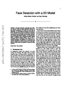
CA ' CA ' CA ' 0 . We see that there are no RG induced axial-vector currents with light quarks. However, the vector currents, with tree-level coefficients equal to one, receive radiative corrections from oneloop diagrams involving the electromagnetic coupling. These corrections are O(1%) for mV ∼ 1 TeV and scale logarithmically with the mediator mass. Although they should be included for a correct evaluation of the rate, they turn out to give only a small effect. The situation is dramatically different for the case of axial-vector couplings to quarks i h αt αb (u) ln(mV /mZ ) − ln(mV /µN ) , Axial-vector to quarks: CV ' 3 − 8s2w 2π 2π i h αt αb (d) 2 CV ' 3 − 4sw − ln(mV /mZ ) + ln(mV /µN ) , 2π 2π (4.10) 3α 3α t b (u) CA ' 1 − ln(mV /mZ ) + ln(mV /µN ) , 2π 2π 3α 3αb t (d) (s) CA ' CA ' 1 + ln(mV /mZ ) − ln(mV /µN ) . 2π 2π The mixing into the light quark vector currents is non-vanishing in this case. The dominant contribution comes from the top Yukawa, and for mV ∼ 1 TeV this gives an O(3 − 5%) coupling to the light quark vector currents. Moreover, the size of the axial-vector coupling to light quarks is also affected. Again, due to the size and the RGE of the top Yukawa, this effect is larger than the approximate expressions in Eq. (4.10), giving corrections of order O(10%) for mV ∼ 1 TeV. We now turn to Fig. 1, which shows the 90% exclusion limits on the mediator mass for fermionic DM, obtained from the null results of the LUX experiments (blue) as well as the projected limits from the LZ experiment (orange). For the case of vector interactions in both the DM and quark sectors (top left), we obtain strong limits on the mediator mass, up to around mV ∼ 20 TeV from LUX. In this benchmark, DM couples to the light quarks at tree level with a standard SI interaction, which is coherently enhanced with the square of the number of nucleons 11

LZ pr oj

ected

LUX 2

10

4

014

103

102 10 106 105 Mediator mass mV [GeV]

Flavor universal: Quarks only χγ ¯ µ χf¯γµ f Mediator mass mV [GeV]

105

104

102 103 Dark Matter mass mχ [GeV]

LZ proje

cted

14

3

102

104 LZ pr ojecte d

103


Flavor universal: Quarks only χγ ¯ µ γ 5 χf¯γµ γ 5 f

104 LZ pr

ojecte d

103 LUX


102 10

104

104

105

10 1 10

LUX 2

014

106

Flavor universal: Quarks only χγ ¯ µ χf¯γµ γ 5 f

Flavor universal: Quarks only χγ ¯ µ γ 5 χf¯γµ f

105

102 10

104

LUX 20

10

106

Mediator mass mV [GeV]


106

2014


104

Figure 1: Experimentally excluded regions in the (mDM , mV ) plane for the case of fermion DM and mediator with flavor universal coupling to quarks (Benchmark I). We shade the LUX 90% excluded region (blue) and also show the projected LZ exclusion (orange). In the two upper panels we consider a mediator coupling to the quark vector current, and on the left (right) we take the coupling to the DM (axial-)vector current. We do the same in the lower panels, where we consider a mediator coupled to the quark axial-vector current. Dashed lines indicate the exclusion limits when the running of the couplings is not considered. Where only solid lines are shown this means that the limits with and without running are indistinguishable.

12

105

LZ pr oj

ected

LUX 2

10

4

106

Flavor universal: Quarks only ↔ φ† ∂ µ φf¯γµ f

105 Mediator mass mV [GeV]


106

014

103

Flavor universal: Quarks only ↔ φ† ∂ µ φf¯γµ γ 5 f LZ proje

cted

104

LUX 20 1

10

4

3

102 10

102 10


1 10

104


104

Figure 2: Same as Fig. 1 but for scalar DM. in the nucleus. For this benchmark, the limits with and without running are indistinguishable. As shown in Eq. (4.9), corrections to the quark vector couplings are driven by electromagnetic interactions and are therefore small. For the same reason, there are no strong running effects when we consider the axial-vector current of DM coupling to the quark vector current (top right). The quark vector current does not mix into the axial-vector current, meaning that the standard SD interaction is not induced. Instead, the DD rate is due to NR operators ONR and ONR (see Appendix C), which 8 9 are suppressed by the DM velocity and the nuclear recoil momentum respectively. Thus, we obtain weaker limits from LUX and LZ when compared with the vector-vector case. For the vector current of DM coupling to the axial-vector current of quarks (bottom left), we obtain very weak limits in the na¨ıve analysis where we neglect operator mixing (dashed lines). Again, this is because the resulting interaction (mediated by operators ONR and ONR defined 7 9 in Appendix C) is velocity and momentum suppressed. However, when we include the effects of mixing (solid lines), the limits are strengthened by around 2 orders of magnitude. As shown in Eq. (4.10), a coupling to the quark vector current is induced. The resulting vector-vector interaction gives rise to SI scattering, meaning that despite this rather small induced coupling, the DD rate is large due to the coherent enhancement. This effect was pointed out previously in Refs. [18, 21] and demonstrates that models which appear to have suppressed DM-nucleon interactions can in fact lead to unsuppressed scattering and therefore much stronger limits. For axial-vector couplings to both DM and quarks (bottom right), DM-nucleon scattering is mediated by the standard SD coupling at tree level. Because there is no coherent enhancement in this case, the limits are weaker than in the vector-vector case (top left). When the effects of running are included, the limits become stronger. Though the mixing of the quark axialvector current with the vector current does lead to a new velocity-suppressed contribution, the dominant effect is in the running of the axial-vector couplings themselves. From the last two lines of Eq. (4.10), we see that the coupling to the up quark is reduced, while the coupling to 13

the down and strange quarks is enhanced. This has the effect of increasing the SD coupling to neutrons, which increases the DD rate in Xenon targets, whose nuclear spin is dominated by the presence of an unpaired neutron. Note, however, that the running also has the effect of decreasing the SD coupling to protons, meaning that for some targets (such as Fluorine) the DD rate will be reduced. Remarkably, this isospin-violation is entirely driven by loops of SM particles and it persists even if the mediator V couples in an isospin-conserving way, as first pointed out in Ref. [18]. We will discuss this effect in more detail in Sec. 6, where we explore complementarity between DD and collider searches. Finally, we consider the limits on this benchmark for scalar DM, shown in Fig. 2. In the left panel, for scalar DM coupling to the quark vector current, we obtain limits identical to those of fermionic DM vector-vector interactions. This is because both interactions reduce to the same non-relativistic operator, namely ONR 1 , the standard SI interaction. For scalar DM coupling to the quark axial-vector current, the results also appear similar to the DM vector-current case. In the scalar case, however, the limits without running (dashed lines) are slightly weaker, due to the fact that only the suppressed operator ONR contributes (see Eq. C.6 in Appendix C). 7 However, once running is taken into account, the standard SI interaction is induced and the limits match those obtained for the fermionic DM vector current. In this section, we have discussed a benchmark in which DM couples to all quarks in a flavor universal way through a vector mediator. In particular, this means that the interactions which mediate DM-nucleon scattering (the couplings to light quarks) appear at tree level in the high energy Lagrangian. However, there are two key effects which arise when the RGE is taken into account. First, the size of these tree level couplings may be altered, as seen in the lower right panel of Fig. 1 for standard SD interactions. Second, new couplings may be induced which, if they lead to unsuppressed DM-nucleon scattering, can lead to much stronger limits. We note in particular that for each of the DM interaction structures we have considered (scalar, vector and axial-vector), the limits coming from couplings to quark vector currents and couplings to quark axial-vector currents are comparable once the running has been accounted for. Though in the standard picture (without running) only one of these interactions is assumed to dominate, here we have demonstrated that both are important and both must be included to give accurate limits on simplified models with vector mediators.

4.2

Benchmark II: flavor universal couplings to leptons

We now consider the opposite case in which all couplings to quarks are switched off, (i)

(i) c(i) q = cu = cd = 0 ,

(i = 1, 2, 3) ,

(4.11)

and interactions between DM and SM involve only lepton fields. We assume flavor universal couplings also in this case, and we are thus left with only two dimensionless couplings: (i)

cl = cl ,

c(i) e = ce ,

(i = 1, 2, 3) .

(4.12)

We present results for the two following choices Vector to leptons: Axial-vector to leptons: 14

ce = cl = 1 , ce = −cl = 1 ,

(4.13) (4.14)

namely for the effective interactions at the mediator mass scale of the form Vector to leptons: Axial-vector to leptons:

LEFT

3 X 1 ei γ µ ei , = − 2 JDM µ mV i=1

(4.15)

LEFT

3 X 1 = − 2 JDM µ ei γ µ γ 5 ei . mV i=1

(4.16)

A peculiar feature of this benchmark is that DD rates are entirely due to RG effects. The contact interactions obtained by integrating-out the mediator particle do not involve light quarks. Thus, the DM-nucleon scattering cross section is only due to radiatively induced interactions with light quarks. The regions excluded in the (mχ , mV ) plane for the 6 possible combinations are shown in Figs. 3 and 4. In order to understand these plots, it is helpful again to look at the approximate analytical solutions. For vector couplings to leptons we have Vector to leptons:

4αem ln(mV /µN ) , 3π 2αem (d) CV ' − ln(mV /µN ) , 3π (u) (d) (s) CA ' CA ' CA ' 0 . (u)

CV '

(4.17)

As we have already found in Eq. (4.9), there is no induced axial-vector couplings to light quarks if the mediator couples only to vector currents. However, unlike the case of Eq. (4.9), there are only RG induced vector couplings to light quarks. These are the main source for DD rates. Likewise, for axial-vector couplings to leptons we have Axial-vector to leptons:

ατ (u) 3 − 8s2w ln(mV /µN ) , CV ' − 6π ατ (d) 3 − 4s2w ln(mV /µN ) , CV ' 6π ατ (u) (d) (s) CA ' −CA ' −CA ' ln(mV /µN ) . 2π

(4.18)

The Yukawa coupling of the τ leptons generates one-loop suppressed couplings to both vector and axial-vector couplings of the low energy current. Turning now to the limits obtained for this benchmark, we see from the top row of Fig. 3 that for fermionic DM, constraints on the mediator mass are roughly an order of magnitude weaker for vector couplings to leptons compared to universal vector couplings to quarks. In the latter case, the running of the couplings had little impact, due to the smallness of the electromagnetic coupling compared to the tree level coupling to the light quarks. In the present case, as can been seen in Eq. (4.17), the radiatively induced coupling to light quarks is the only contribution. This RG-induced coupling is at the percent level, meaning that mV must be reduced by a factor of roughly 10 to achieve the same DD cross section as in the universal quark coupling case (as the cross section scales as ∼ C2 /m4V ). For couplings of fermionic DM to the axial-vector current of leptons (bottom row of Fig. 3), the limits are now roughly two orders of magnitude weaker than in the case of couplings to quarks. Once again, the only contribution to the DD rate is due to RG effects. However, the effect of the running is smaller for the lepton benchmark than for the quark benchmark. In 15


105

106

Flavor universal: Leptons only χγ ¯ µ χf¯γµ f

104

LZ proje cted

103

LUX 201


106

4

102 10

106


105


1 10

102

LZ proje

cted

LUX 20

106

Flavor universal: Leptons only χγ ¯ µ χf¯γµ γ 5 f

103

10

103

1 10

104

104

102

104

14

10

LZ proje

cted

LUX 2

014



1 10

Flavor universal: Leptons only χγ ¯ µ γ 5 χf¯γµ f

104

Flavor universal: Leptons only χγ ¯ µ γ 5 χf¯γµ γ 5 f

104 103 102 10 1 10

104


LZ pr ojecte

d


104

Figure 3: Same as Fig. 1 but for flavor universal couplings to leptons (Benchmark II). In all cases, no limits are obtained when running of the couplings is not taken into account.

16

106

104

LZ proje cted

103

LUX 201

4

102

Flavor universal: Leptons only ↔ φ† ∂ µ φf¯γµ γ 5 f



106

Flavor universal: Leptons only ↔ φ† ∂ µ φf¯γµ f

104 103 LZ proje cted

102

10

LUX 2

014

10

1 10


1 10

104


104

Figure 4: Same as Fig. 3 but for scalar DM. the latter, the running is driven by the top Yukawa, while in the former, the running is driven predominantly by the smaller τ Yukawa (Eq. (4.18)). For axial-vector couplings to both DM and leptons (lower right panel of Fig. 3), we note that we obtain no limits from LUX above a mediator mass of 1 GeV and only very weak limits projected for LZ. We also note that at low and high mass, the projected LZ limits appear to drop off rapidly. For mediator masses close to 1 GeV, the running is too small to produce an observable DD signal and therefore no limits are obtained. However, we stress that the formalism used for the RGE (which involves resumming loop contributions proportional to Log[mV /µN ]) is likely to break down as we approach mV = µN . The limits obtained with this formalism therefore cannot necessarily be trusted for mV ∼ 1 GeV. Finally, for scalar DM (Fig. 4), the limits are very similar to those of fermionic DM with vector-current interactions, as discussed for Benchmark I. We highlight once again that these scalar DM interactions with leptons would lead to no DD constraints in a na¨ıve treatment, but can give substantial constraints once RG effects are accounted for (especially in the case of coupling to lepton vector currents).

4.3

Benchmark III: couplings to third generation

Our last case involves coupling to only the third generation of SM fermions i3 (3) c(i) q = δ cq , (i)

(3)

cl = δ i3 cl ,

cu(i) = δ i3 c(3) u ,

(i)

(3)

cd = δ i3 cd ,

i3 (3) c(i) e = δ ce

(i = 1, 2, 3) .

(4.19)

We choose again two benchmark models with purely vector or axial-vector couplings Vector to 3rd: Axial-vector to 3rd:

(3)

(3)

(3) c(3) u = cd = cq = cl (3)

(3)

(3) c(3) u = cd = −cq = cl

17

= c(3) e = 1, = −c(3) e = 1.

(4.20) (4.21)

The associated effective Lagrangian features only DM interactions with the top and bottom quarks and the τ lepton Vector to 3rd: Axial-vector to 3rd:

1 JDM µ m2V 1 = − 2 JDM µ mV

LEFT = −

tγ µ t + bγ µ b + τ γ µ τ ,

(4.22)

LEFT

tγ µ γ 5 t + bγ µ γ 5 b + τ γ µ γ 5 τ .

(4.23)

The exclusion limits for these benchmarks are shown in Figs. 5 and 6, but we once again examine the approximate analytical expressions for the couplings before looking at the bounds in detail. As was the case for the lepton benchmarks, this case has DD rates due entirely to radiatively induced interactions. An interesting effect happens for the case of vector couplings: above the weak scale the contribution from quarks is exactly canceled by the one from leptons. This can be understood by noticing that the effect is driven by electromagnetic loops of heavy fermions, with total contribution proportional to X 2 1 (f ) − −1=0 . (4.24) Nc Qf = 3 × 3 3 f =t,b,τ (f )

Here, Qf is the electromagnetic charge of f and the number of colors is Nc = 3 (1) for quarks (leptons). We are only left with the RGE below the weak scale, non-vanishing now since the top quark is integrated-out. The net result is an induced coupling to vector currents of light quarks: Vector to 3rd:

8αem ln(mZ /µN ) , 9π 4αem (d) ln(mZ /µN ) , CV ' − 9π (u) (d) (s) CA ' CA ' CA ' 0 . (u)

CV '

(4.25)

Although smaller than the couplings in the lepton case in Eq. (4.17) due to less RG evolution, these contributions are still sizable and able to be probed by current and future experiments. Finally, we consider the axial-vector case. Since the effect is driven by SM Yukawa interactions, the low-energy couplings are just the sum of the RG induced ones in Eqs. (4.10) and (4.18) Axial-vector to 3rd:

αt 3 − 8s2w ln(mV /mZ )+ 2π h αb ατ i − 3 − 8s2w + ln(mV /µN ) , 2π 6π αt (d) CV ' − 3 − 4s2w ln(mV /mZ )+ 2π h αb ατ i 3 − 4s2w + ln(mV /µN ) , 2π 6π 3αt (u) (d) (s) CA ' −CA ' −CA ' − ln(mV /mZ )+ 2π 3αb ατ ln(mV /µN ) + ln(mV /µN ) . 2π 2π (u)

CV '

18

(4.26)


105 104 103

106

Third Generation χγ ¯ µ χf¯γµ f

LZ project


106

ed

LUX 2014

102 10

106


105 104


102

106

Third Generation χγ ¯ µ χf¯γµ γ 5 f LZ proje c

ted

14

3

102

105

10 1 10

103

1 10

104

LUX 20

10

104

10


1 10

103

LUX 20 14


104

Third Generation χγ ¯ µ γ 5 χf¯γµ γ 5 f

LZ pro

jected

102

1 10

104

LZ project ed

104

10


Third Generation χγ ¯ µ γ 5 χf¯γµ f

LUX 2

014


104

Figure 5: Same as Fig. 1 but for couplings to third generation fermions (Benchmark III). In all cases, no limits are obtained when running of the couplings is not taken into account.

19


105 104 10

3

106

Third Generation ↔ φ† ∂ µ φf¯γµ f

LZ project

ed

LUX 2014

102 10 1 10

Third Generation ↔ φ† ∂ µ φf¯γµ γ 5 f


106

LZ proje c

104

ted

LUX 20

14

10

3

102 10


1 10

104


104

Figure 6: Same as Fig. 5 but for scalar DM. The limits on the mediator mass in this benchmark are shown in Fig. 5 in the case of fermionic DM. For vector couplings to the third generation fermions (top row), the limits are slightly weaker than those obtained in the lepton-only benchmark (Fig. 3). As already discussed, there is no running above the weak scale in the former case, meaning that the radiatively induced couplings are smaller. In contrast, for axial-vector couplings to third generation fermions (bottom row of Fig. 5), the constraints are substantially stronger when compared to the leptons-only benchmark. This is because the DM couples to all 3 heavy fermions (t, b, τ ) and not just the τ as in the leptonsonly case. As the mixing is driven by the Yukawa couplings, this enhances the RG effects and strengthens the limits. This is perhaps most obvious in the case of scalar DM (Fig. 6), where coupling to the axial-vector current now gives stronger constraints than coupling to the vector current. The DD rate in both cases is dominated by the same low-energy operator (the SI operator ONR 1 ), indicating that the mixing into the light quark vector current must be larger in the case of axial-vector interactions at high-energy. We finally comment on the fact that the LZ projected limits are substantially stronger than the current LUX limits in the case of axial-vector axial-vector couplings to the third generation fermions (lower right panel of Fig. 5). A na¨ıve comparison of the LUX and LZ exposures would suggest that LZ should only be able to constrain mediator masses of mV & 100 GeV. However, as the mediator mass increases above the weak scale, the effects of the running become more significant. The top quark has been integrated out below the Z mass, while it is still in the spectrum (and contributes to the running) above the Z mass. This increases the RG-induced couplings to the light quark axial-vector currents and thus leads to stronger limits on mV .

20

5

Rescaling and general limits

We have so far focused only on a small number of benchmark scenarios. In this section we summarize the procedure for obtaining limits on general vector mediator models with arbitrary coefficients. The public code runDM, released with this paper and available at this http URL, allows the user to evolve the Wilson coefficients of the simplified model between two arbitrary energy scales. The coefficients at the nuclear scale can then be fed into NRopsDD, available at this http URL, which allows the user to derive bounds from current direct detection experiments.3 The procedure is as follows: 1a. Define your favorite model according to the Lagrangian in Eq. (B.1). This amounts to specifying a 16-dimensional array of Wilson coefficients defined in Eq. (B.2), which can be used as input for the runDM code. 1b. Use the function DDCouplingsQuarks to compute the low-energy couplings to light quarks (u, d, s) relevant for direct detection. These should then be dressed to the nucleon level by means of Eq. (3.4), and matched onto the NR operator coefficients (making sure to include all relevant operators, which may not be limited to the standard SI and SD interactions defined in Eq. (3.5)). In order to facilitate this, we also provide the function DDCouplingsNR (N ) which returns the NR coefficients cφ(χ) i , defined in Appendix C, for each type of DM current considered in this work. These coefficients are functions of the coupling of the DM current defined in Eq. (4.1), 16 Wilson coefficients of Eq. (B.1), the DM mass mχ and the mediator mass mV . For compactness, we define λ ≡ (gφ(χ) , 16 Wilson coefficients, mV ). The function DDCouplingsNR automatically performs the embedding of the quark-level couplings to the nucleon level and computes the NR DM-nucleon matrix element according to the numbering of the NR operators defined in Appendix C. 2a. Calculate the benchmark DD coupling λB as a function of the parameters λ and mχ : X X (N ) (N 0 ) (N,N 0 ) (mχ ) = λB (mχ )2 , for scalar DM , cφ i (λ, mχ ) cφ j (λ, mχ ) Yi,j i,j=1,7 N,N 0 =p,n

X

X

i,j=4,8,9

N,N 0 =p,n

X

X

i,j=1,4,7,8,9

N,N 0 =p,n

(N )

(N 0 )

(N,N 0 )

(mχ ) = λB (mχ )2 ,

for Majorana DM ,

(N )

(N 0 )

(N,N 0 )

(mχ ) = λB (mχ )2 ,

for Dirac DM .

cχ i (λ, mχ ) cχ j (λ, mχ ) Yi,j

cχ i (λ, mχ ) cχ j (λ, mχ ) Yi,j

(5.1) (N,N 0 )

Here Yi,j (mχ ) are the rescaling functions computed in NRopsDD, which relate the DD rates for different NR operators. The sum in i, j is over the specific NR operators relevant in each case. 2b. Insert the above expression for λB into the test statistic function TS(λB , mχ ), provided in NRopsDD, for a given DD experiment. At this point the user possesses the test statistic TS(λ, mχ ) and can derive a bound on λ (or equivalently mV ) at the desired confidence level, e.g. by drawing a contour plot of TS = 2.71 for a 90% CL. 3

As part of the runDM release, we also provide an example mathematica notebook illustrating how to interface the two codes.

21

10−37

10−37 LU X2

102

103

−40

10−41 ATLAS monojet

10−42 10−43

σSD (DM-neutron) [cm2 ]

σSD (DM-proton) [cm2 ]

10

ATLAS monojet (with running)

1

10

102

016

1

10−39

X2

10−43

10−42

LU

-2L

10−39 10

10−38

10−42

6 01

CO PI

10−38

10

1

10

102

103

−40

10−41

ATLAS monojet (with running)

10−42

gq = 0.25, gχ = 1.0

ATLAS monojet

Axial Vector Mediator

103

10−43

10−43

104

Dark Matter mass mχ [GeV]

gq = 0.25, gχ = 1.0 Axial Vector Mediator

1

10

102

103

104

Dark Matter mass mχ [GeV]

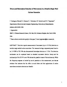
Figure 7: 90% confidence limits on the DM-proton (left) and DM-neutron (right) spindependent scattering cross section for Dirac DM. The dashed green lines show the limits from the ATLAS monojet search at 13 TeV, as reported in Ref. [60], assuming a universal coupling to all quarks through the axial-vector operator χγ µ γ 5 χqγµ γ 5 q. Solid green lines show the correct limits when running of the couplings is taken into account. The inset shows a zoom-in of the ATLAS limits at small cross section. Direct detection limits from LUX [56] (blue) and PICO-2L [61] (red) are also shown for comparison. The coupling gχ used by the LHC collaborations corresponds in this context to our cχA of Eq. 2.4.

6

Connecting direct detection and collider searches

We now turn to an example where the techniques we have developed are important for a correct exploration of the complementarity between different DM searches. Using simplified models, it is possible to map LHC constraints on the mass of the mediator onto the (mχ , σχN ) plane which is usually presented by DD experiments [59]. However, the large separation of scales and resulting RG effects are not typically included in such a mapping. As we will now show, these effects can have a non-trivial effect on the derived cross section limits. The simplified models used in DM searches at the LHC typically assume a universal coupling of the mediator to quarks, corresponding exactly to our Benchmark I, discussed in Sec. 4.1. When the mediator is assumed to couple to the vector current of both DM and quarks, we have seen that the DD rate will not be substantially affected by RG effects. This is because the rate is dominated by the tree level coupling to the light quark vector currents, for which the running is small. In this case, then, the comparison between LHC and DD limits is relatively straightforward. However, for axial-vector current interactions, the running is driven by the top Yukawa and therefore gives a larger effect. As discussed in Sec. 3, interactions of the form χγ µ γ 5 χqγµ γ 5 q lead to a spin-dependent (SD) interaction which is not suppressed by powers of the momentum transfer or the DM speed. In Fig. 7, we show the 90% limits on the DM-proton (left panel) and DM-neutron (right panel) SD cross sections reported by the LUX [56] (blue) and PICO-2L [61] 22

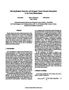
(red) direct detection experiments. On the same plane, we show limits from a recent Run-2 monojet search at ATLAS [60], interpreted in the context of an axial-vector mediator simplified model. The dashed green line shows the limit reported in Ref. [60], without including the effects of running. The solid green line shows the limit when the RG effects discussed in this paper are included. The limits including running are obtained by first taking the reported limits (dashed line) and calculating the corresponding limit on the mediator mass. We then run the couplings from this mediator mass down to the nuclear scale and calculate the SD cross section (see Eq. (6.1)). The difference is a factor of approximately 2 in the cross section, with the limits being strengthened in the DM-proton case and weakened in the DM-neutron case. In order to understand this difference, we need the explicit expression for the DM-nucleon SD cross section (in the zero momentum transfer limit) shown in Eq. (3.5). Combining Eqs. (4.10) and (3.4), we see that at the nuclear energy scale, the axial couplings to nucleons can be written, " (N )

CA = gq

# X

) ∆(N + q

q=u,d,s

3gq (N ) ) (N ) [αt ln(mV /mZ ) − αb ln(mV /µN )] , (6.1) − ∆ ∆d + ∆(N s u 2π

(N )

where the axial-charges ∆q are defined in Eq. (3.4). We have also explicitly included the coupling of the mediator to quarks gq to allow for the possibility that this may differ from unity. The first term (in square brackets) is the DM-nucleon coupling evaluated at the energy scale of the mediator and leads to equal couplings to protons and neutrons. The second term in Eq. 6.1 accounts for RG effects, which induce a correction to the up quark current with an (p) (n) opposite sign to the corrections for down and strange quarks. Noting that ∆u = ∆d and (p) (n) ∆d = ∆u , we see that the corrections to the nucleon couplings will have roughly opposite signs for protons and neutrons.4 This is illustrated in Fig. 8, where we show the proton and neutron SD cross sections as a function of the mediator mass. For each value of the mediator mass, we normalise the cross section relative to its na¨ıve value without taking running into account. The origin of the differences in Fig. 7 is now clear; the running of the couplings enhances the DM-neutron coupling, leading to weaker limits from the LHC (and vice-versa for DM-proton couplings). It should also be clear from this plot that any choice of the ratio between DM-neutron and DMproton couplings at the nuclear energy scale must necessarily be fine tuned in this framework. The seemingly natural choice of equal SD couplings to protons and neutrons will correspond to a different choice of couplings at the energy scale of the mediator. In other words, running of the couplings will naturally induce isospin-violation for SD couplings [18, 21]. We have focused here on the case of axial-vector couplings, finding that the mapping from LHC limits to the DD plane should be corrected by a factor of roughly 2 when including the effects of running. However, in some cases, the standard lore is that LHC limits on the mediator mass cannot be mapped onto DD limits, as the corresponding DD rate is small. Interactions of the form χγ µ γ 5 χqγµ q and χγ µ χqγµ γ 5 q lead to velocity- and momentum-suppressed rates in DD experiments and are therefore not expected to be competitive with DD limits. However, as we have shown in Sec. 4.1, mixing effects can induce substantial rates which are comparable to or even greater than the standard SD rate (see Fig. 1). In these cases, the inclusion of RG effects is therefore essential for a correct comparison between the LHC and DD results. 4

(N )

The contribution from ∆s

is smaller though not negligible.

23

N N σSD (with running)/σSD (without running)

2.5 Flavor universal: Quarks only χγ ¯ µ γ 5 χf¯γµ γ 5 f 2.0 ut ne

n ro

1.5

1.0 pro

ton

0.5

0.0 10

102 103 104 Mediator mass mV [GeV]

105

Figure 8: Spin-dependent (SD) DM-nucleon cross section as a function of the mediator mass mV , normalised to the value obtained when the running is not considered. Results for the DM-neutron cross section are shown in magenta, while the DM-proton cross section is shown in cyan. We assume that at high energy DM couples universally to all quarks through the axial-vector interaction χγ µ γ 5 χf γµ γ 5 f .

7

Conclusions

In this work, we have performed a systematic study of the direct detection of SM-singlet DM which interacts with SM fermions through the exchange of a heavy vector mediator. We have considered both scalar and fermion DM with general, gauge-invariant couplings to SM fermions. We have also taken into account all relevant non-relativistic DM-nucleon interactions in order to obtain current and projected limits on the mass scale of the mediator. Most importantly, however, we have accounted for RG effects connecting the couplings defined at high energy and those relevant for low-energy DM-nucleon scattering. If the mediator couples universally to all quarks (Sec. 4.1), there are two key effects. The first is to change the size of the couplings at low energy with respect to the values defined at the energy scale of the mediator mass. When the mediator couples to quark vector currents, this effect is driven by electromagnetic loops and is therefore small. In contrast, if the mediator couples to quark axial-vector currents, the effect is dominated by the top Yukawa and is therefore larger. This effect is most pronounced when DM also couples through the axial-vector current, leading to spin-dependent DM-nucleon scattering. The second effect is operator mixing, inducing new interactions at low energy that are not present at high energy. Though the size of the mixing may be relatively small, the DD rate can be increased by several orders of magnitude if the new interaction is not suppressed by powers of the velocity or momentum-transfer. For couplings to quarks, the result is that irrespective of the DM spin and interaction structure, DD experiments can always exclude mediators lighter than mV ∼ 200 GeV, and in some cases this exclusion extends up to mV ∼ 10 TeV. 24

In cases where the mediator does not couple to light quarks, DM-nucleon scattering is not possible at tree level. However, SM loops generically induce these couplings, allowing DD experiments to set limits on such models, as demonstrated in Sec. 4.2 and 4.3. Such limits are typically stronger if the mediator couples to the top quark axial-vector current, due to the large top Yukawa coupling giving large mixing effects. The only model we have considered which is not constrained by current DD experiments is the case in which the mediator couples to the axial-vector currents of both the DM and SM leptons. However, even in this case, future experiments such as LZ should be able to explore such models. Of course, the benchmarks we have considered are not exhaustive. However, they have allowed us to highlight the key features which appear when the running of operators is correctly accounted for. For more general sets of couplings, Sec. 3 gives the recipe for connecting the high energy Lagrangian with the low-energy DD observables. A key ingredient in this recipe, the low-energy light quark couplings as a function of the mediator mass, is approximately given by the analytical expressions in Appendix A. We also distribute together with this work the code runDM, which can be downloaded at this http URL, with which a more rigorous RGE can be performed. Once we have derived the low-energy couplings, exclusion limits for any arbitrary choice of couplings can be obtained by adopting the rescaling procedure described in Sec. 5. We emphasise once again that these RG effects arise only from SM loops and are therefore not optional. The tools we provide should facilitate the inclusion of these effects in all future studies of vector mediated simplified models. Finally, we have briefly examined the comparison between LHC and DD limits. We have found that for the case of a mediator with axial-vector interactions, LHC bounds translated into the (mχ , σχN ) plane can be altered by a factor of 2 when the effects of running are included. For interactions which na¨ıvely give no limits in DD experiments, we have also demonstrated that operator mixing can have a significant impact, meaning that LHC limits on such interactions can in fact be complementary to DD searches. We urge the LHC experimental collaborations to include these effects when comparing with DD experiments in order to correctly map the complementarity between the different search strategies.

Acknowledgments The authors thank J. Silk and F. Sala for discussions and S. Profumo for helpful comments on this manuscript. FD thanks J. Silk for his kind hospitality at the Institut d’Astrophysique de Paris where part of this work was completed. PP thanks S. Profumo for his kind hospitality at UC Santa Cruz, where this work was initiated. FD is supported by the U.S. Department of Energy grant number DE-SC0010107 (FD). P.P. acknowledges support of the European Research Council project 267117 hosted by Université Pierre et Marie Curie-Paris 6, PI J. Silk. BJK is supported by the John Templeton Foundation Grant 48222 and by the European Research Council (Erc) under the EU Seventh Framework Programme (FP7/2007-2013)/Erc Starting Grant (agreement n. 278234 — ‘NewDark’ project).

A

A simple analytical solution for the RGE

The complete procedure to properly connect the energy scales is rather involved, as described in the first part of Sec. 3. The study for the three benchmark models in Sec. 4 was performed 25

by implementing the full RGE without any approximation. Our results in Figs. 1 to 6 can be qualitatively understood with the help of analytical equations expressing the low-energy couplings in terms of the ones at high-energy. Furthermore, general analytical solutions make it easy to estimate the size of these RG effects. Providing these simple equations is the goal of this appendix. The accuracy of these approximate solutions is quantified in Appendix B for the benchmark model of a mediator coupled to quarks, where RG effects are maximal due to the large top Yukawa coupling. A more refined study can be performed by using the public code released with this work. We start by quantifying the approximations made to derive the analytical expressions given in this Appendix. The system of RG equations as given in Ref. [21], both above and below the EWSB scale, schematically reads dci (µ) = γij (µ)cj (µ) . d ln µ

(A.1)

Here, µ is the renormalization scale and ci is an array of Wilson coefficients. The entries of the anomalous dimension matrix γij (µ) are numerical coefficients and SM couplings. The renormalization scale dependence in the anomalous dimension matrix can only be implicit through the running SM couplings, since we work in a mass independent scheme (MS). Our first approximation is to ignore the scale dependence of the SM couplings, and we take them evaluated at the renormalization scale µ = mZ .5 The RG system becomes dci (µ) (0) = γij cj (µ) , d ln µ

(A.2)

(0)

where γij = γij (mZ ). The linear system in Eq. (A.2) can be solved analytically, since exp −γ (0) ln µ ij cj (µ) = const .

(A.3)

It is straightforward to check the validity of this result by taking the derivative with respect to d ln µ and then using Eq. (A.2). This relation allows a simple connection between the couplings cj (µ) at two different scales. However, it involves the exponential of the anomalous dimension, which is a 16 × 16 matrix [21], and therefore it cannot be translated into simple analytical equations. We make one further approximation: Taylor expand the exponential 1 − γ (0) ln µ ij cj (µ) = const . (A.4) This is justified as long as we do not have large logarithms in our solution. The largest entry in the anomalous dimension matrix is the one proportional to the square of the top Yukawa coupling, therefore our approximation is valid as long as 3

λ2t ln(mV /mZ ) 1 . 8π

(A.5)

In spite of the complicated initial RG system, these two approximations yield an extremely simple final result. Here, we give the low-energy couplings appearing in the effective Lagrangian 5

This is the approximation made in Appendix D of Ref. [21]. Here, we push this approximation one step further as described in the following.

26

in Eq. (3.2) defined at the nuclear scale µN , since they are the only ones relevant to the calculations of direct detection rates. We consider the most general choice of SM couplings to the mediators, namely we keep the 15 couplings appearing in Eq. (2.6) completely general. For each coupling, the final result takes the form (u,s,d) (u,s,d) (u,s,d) (u,s,d) CV,A = CV,A + CV,A + CV,A . (A.6) tree

e.m.

Yukawa

The tree-level contribution, if present, is the coupling we would have without considering RG effects. The two other terms are one-loop interactions induced by the RGE, and within our approximation their effects are driven by electromagnetic and Yukawa interactions. We start from vector currents, with direct detection rates only sensitive to the coupling to the up and down quarks. For the up quark we have the induced coupling at low-energy (1) (1) cq + cu (u) , CV = 2 " tree ! ! # 2 (3) (3) (i) (i) X αem cq + cu cq + cu (u) CV = −8 ln(mV /mZ ) + ln(mV /µN ) + 9π 2 2 e.m. i=1 " # 3 (i) (i) (i) (i) αem X cq + cd cl + ce 4 + ln(mV /µN ) , (A.7) 9π i=1 2 2 ! (3) (3) α −c + c q u t (u) = (3 − 8s2w ) CV ln(mV /mZ )+ 2π 2 Yukawa ! !# " (3) (3) (3) (3) −c + c α −c + c α q e τ b d l − (3 − 8s2w ) + ln(mV /µN ) . 2π 2 6π 2 The tree-level coupling in the first equation is already present at the mediator scale mV . The first row of the one-loop induced coupling driven by electromagnetic interactions has contributions from the up-type quarks. The top quark effects are only present down to the weak scale, since for lower energies the top is not a propagating degree of freedom. In the second row of the electromagnetic term we have contributions to the RGE by the down-type quarks and leptons. The Yukawa terms are dominated by third generation fermions, and again the RG driven by the top quark only contributes down to the weak scale. Likewise, for the down quark we have (1) (1) cq + cd (d) CV = , 2" tree ! ! # 2 (3) (3) (i) (i) X c + c c + c α q u q u em (d) ln(mV /mZ ) + ln(mV /µN ) + CV =4 9π 2 2 e.m. i=1 " # 3 (i) (i) (i) (i) αem X cq + cd cl + ce + ln(mV /µN ) , −2 (A.8) 9π i=1 2 2 ! (3) (3) α −c + c q u t (d) CV =− (3 − 4s2w ) ln(mV /mZ )+ 2π 2 Yukawa " ! !# (3) (3) (3) (3) α −c + c α −c + c q e b τ d l (3 − 4s2w ) + ln(mV /µN ) . 2π 2 6π 2 27

We now consider the induced axial-vector currents of light quarks. The solutions are even simpler for these cases, since the electromagnetic effects are absent (u,d,s) CA =0. (A.9) e.m.

For the up quark we have the following tree-level and Yukawa terms (1)

(u) CA

(u) CA

tree

Yukawa

(1)

−cq + cu = , 2 ! (3) (3) αt −cq + cu = −3 ln(mV /mZ )+ 2π 2 " ! !# (3) (3) (3) (3) αb −cq + cd ατ −cl + ce 3 + ln(mV /µN ) . 2π 2 2π 2

(A.10)

Likewise, for the down and strange quarks we have (d) CA

(1)

tree

(s) CA tree (d) CA Yukawa

(1)

−cq + cd , 2 (2) (2) −cq + cd , = 2 (u) (s) = − CA = CA

=

Yukawa

(A.11)

Yukawa

.

The RG induced couplings driven by Yukawa interactions are the same for the down and the strange quarks, and they are the opposite of the one for the up quark. A few comments are in order. The relations in Eqs. (A.7)-(A.11) are approximate: the running of the SM couplings is neglected and the logarithms in Eq. (A.4) are not re-summed (as instead they are in Eq. (A.3)). The error made by using these solutions is quantified in Appendix B. Furthermore, the above equations are only valid for mV > mZ . For mediator mass below the weak scale, we cannot consider the coupling to the top quark, since it is not consistent to integrate-out the mediator and keep the top quark in the spectrum. The above equations can still be used for mV < mZ , but without the contributions arising from loops of the top quark. In this case, the effective couplings defined at the scale mV are understood as arising from integrating-out the mediator V and the heavy SM degrees of freedom. We conclude this appendix by rewriting the analytical solutions in terms of vector and axial-vector currents of SM fermions as given in Eq. (2.7). We emphasize again that this choice is not gauge invariant, and the couplings have to respect the conditions listed in Eq. (2.8). Nevertheless, it is still useful to rewrite the solutions within this language, since they take a particularly simple form. The low-energy vector current of up quark reads (u) (1) CV = cV u , tree " ! # 2 3 X αem (3) 1 X (i) (i) (i) (u) CV = −8 cV u ln(mV /mZ ) + cV u − c + cV e ln(mV /µN ) , 9π 2 i=1 V d e.m. i=1 hα αt ατ (3) i b (3) (u) (3) CV = (3 − 8s2w )cAu ln(mV /mZ ) − (3 − 8s2w ) cAd + c ln(mV /µN ) . 2π 2π 6π Ae Yukawa (A.12) 28

The one for the down quarks reads (d) (1) CV = cV d , tree " ! # 2 3 X αem (3) 1 X (i) (d) (i) (i) CV =4 cV u ln(mV /mZ ) + cV u − c + cV e ln(mV /µN ) , 9π 2 i=1 V d e.m. i=1 hα ατ (3) i αt b (3) (3) (d) (3 − 4s2w )cAu ln(mV /mZ ) + (3 − 4s2w ) cAd + c ln(mV /µN ) . CV =− 2π 2π 6π Ae Yukawa (A.13) The expression for the low-energy axial-vector currents are even simpler (u) (1) CA = cAu , tree h α αt (3) ατ (3) i b (3) (u) CA = − 3 cAu ln(mV /mZ ) + 3 cAd + c ln(mV /µN ) , 2π 2π 2π Ae Yukawa

(A.14)

and

(d) CA

(1)

tree

(s) CA

(d) CA

tree

Yukawa

= cAd , (2)

= cAd , (s) = CA

(A.15) Yukawa

(u) = − CA

Yukawa

.

for up and down quarks, respectively. The usefulness of the solutions as in Eqs. (A.12)-(A.15), other than being manifest expressions for the low-energy couplings in the benchmark discussed in Sec. 4, consists in providing us with a simple vademecum to quantify RG effects. If the mediator couples to vector currents of SM fermions, RG effects only generates vector currents to light quarks at low-energy. If this is the case, these effects are relevant only if the mediator does not couple to light quarks at tree-level (e.g. leptophilic, heavy quarks), otherwise we only have O(1%) corrections to the couplings, since the effect is driven electromagnetic interactions. On the contrary, if the mediator couples to axial-vector currents of SM fermions, RG effects generate both vector and axialvector currents with light quarks at low-energy. In this case the effects is driven by Yukawa couplings, therefore it is dominated by loops of heavy SM fermions.

B

runDM: a code for the RGE

We release together with this paper the public code runDM. This code can RG evolve the Wilson coefficients of the simplified models discussed in this work between two arbitrary energy scales. As a specific application, runDM can evolve the couplings from the mediator mass scale down to the nuclear scale and provide us with the low-energy couplings relevant to direct detection rates. The code is available at this http URL together with its documentation. In this appendix we describe how the RGE is implemented in runDM. We conclude by comparing the output of the code with the full numerical solution of the RG system and the analytical solutions provided in Appendix A. We perform the comparison in the first benchmark model discussed in this work, where RG effects are maximal due to the large top Yukawa coupling. 29

We find that runDM reproduces the full results with extreme accuracy, and we quantify the error made by using the analytical expressions. Following the framework developed in Ref. [21], the RGE is divided in two regimes, above and below the EWSB scale. At energy scale above the Z boson mass, the effective interactions between DM and SM are described by the Lagrangian (µ>m ) LEFT Z

3 1 µ X (i) i µ i (i) i µ i i µ i = − 2 JDM cq qL γ qL + c(i) u γ u + c d γ d u R R + R R d mV i=1

(B.1)

3 ← → 1 µ 1 µ X (i) i µ i i µ i e γ e − 2 JDM JDM cH H † i D µ H . cl lL γ lL + c(i) e R − R 2 mV mV i=1

Although we have always assumed cH (mV ) = 0 throughout this work (i.e. that the mediator is not coupled to the Higgs), runDM can deal with this more general case as well. We organize the Wilson coefficients in the 16-dimensional array cT (µ) =

(1)

cq

(1)

cu

(1)

cd

(1)

cl

(1)

ce

(2)

cq

(2)

cu

(2)

cd

(2)

(2)

cl

ce

(3)

cq

(3)

cu

(3)

cd

(3)

cl

(3)

ce

cH

,

(B.2)

and the connection between the couplings at two different energy scales (both above the Z boson mass) can be found by solving the system of RG equations dc = γSMχ c . d ln µ

(B.3)

The explicit form of γSMχ can be found in Ref. [21]. Likewise, at energies below the EWSB scale we have the effective couplings (µN ) LEFT

2 3 i 1 µ X (i) i µ i 1 µ X h (i) i µ i (i) = − 2 JDM CV u u γ u − 2 JDM CV d d γ d + CV e ei γ µ ei + mV mV i=1 i=1 2

(B.4)

3

i 1 µ X h (i) i µ 5 i 1 µ X (i) i µ 5 i (i) CAd d γ γ d + CAe ei γ µ γ 5 ei . CAu u γ γ u − 2 JDM − 2 JDM mV mV i=1 i=1 In the above equation there is no contribution from the top quark couplings, since at such low energy scales the top is integrated out. The Wilson coefficients in the above Lagrangian can be arranged in the array CT (µ) =

(1)

CV u

(1)

CV d

(2)

CV u

(2)

CV d

(3)

CV d

(1)

CV e

(2)

CV e

(3)

CV e

(1)

CAu

(1)

CAd

(2)

CAu

(2)

CAd

(3)

CAd

(1)

CAe

(2)

CAe

(3)

CAe

. (B.5)

The connection between the couplings at two arbitrary energy scales below the Z boson mass is achieved by solving the RG system dC = γEMSMχ C , d ln µ

(B.6)

where the explicit form of γEMSMχ can also be found in Ref. [21]. If we want to connect two energy scales above and below the Z boson mass, there is a further intermediate step: a matching between the two EFTs at the EWSB scale. This is obtained by C(mZ ) = Umatch c(mZ ) , 30

(B.7)

where the explicit form for Umatch is given in Ref. [21]. The RG systems in Eqs. (B.3) and (B.6) allow for a connection between two arbitrary energy scales in each EFT. We formally define the evolution matrix USMχ (µa , µb ) above the EWSB scale, which evolves the array of Wilson coefficients in Eq. (B.2) from the energy scale µb to the energy scale µa . More explicitly, the evolution matrix acts as follows c(µa ) = USMχ (µa , µb ) c(µb ) .

(B.8)

We define the analogous quantity UEMSMχ (µa , µb ) for the RG evolution below the EWSB scale. The general evolution matrix between two arbitrary energy scale thus reads  µa , µb > mZ  USMχ (µa , µb ) UEMSMχ (µa , mZ ) Umatch USMχ (mZ , µb ) µa < mZ < mb . U (µa , µb ) = (B.9)  UEMSMχ (µa , µb ) Umatch µa , µb < mZ In the above equation, we assume the boundary condition at µb to be expressed in terms of the array in Eq. (B.2), and the final output at µa in terms of the array in Eq. (B.2) (Eq. (B.5)) for µa greater (smaller) than the Z boson mass. This is the reason why we include the matrix Umatch in the last row of the above equation. As a specific application, we can run from the mediator mass scale down to the nuclear scale µN , and we have the evolution matrix UEMSMχ (µN , mZ ) Umatch USMχ (mZ , mV ) mV > mZ UDD (mV ) = . (B.10) UEMSMχ (µN , mV ) Umatch mV ≤ mZ All we have left to do is to evaluate the evolution matrices. We follow the prescription given in Appendix C of Ref. [21], where the running of SM couplings was treated as a perturbation. The set-up is formally identical to time-dependent perturbation theory in quantum mechanics, where the running of SM couplings acts as the potential interaction. The system can be solved by defining the equivalent of the “interaction-picture” variables, and expressing the solution of the resulting “Schwinger-Tomonaga” equation in terms of a Dyson series. We produce evolution matrices accounting for the running SM couplings up to the 1st order in the Dyson series. These are the evolution matrices used by runDM. We conclude this Appendix with a comparison among different methods to solve the system of RG equations. The purpose of this test is twofold: validate the evolution matrices used by runDM and quantify the accuracy of the analytical solutions given in Appendix A. We perform the comparison in the benchmark model where the mediator is coupled to quarks only, and we take flavor universal couplings. This is the case where RG effects are expected to be maximal, as a consequence of the large top Yukawa coupling. We consider both vector and axial-vector couplings, and we solve the RG system with 3 different methods: the full solution by solving the differential equations of the RG system, the analytical solutions in Appendix A and the solution to the “Schwinger-Tomonaga” equation up to the 1st order in the Dyson series. We start from couplings to quark vector currents as given in Eq. (4.5). In this case there are no induced axial-vector currents at low-energy. We focus on the induced vector currents, which have both a tree-level part as well as a one-loop RG contribution driven by electromagnetic interactions. We show results in Fig. 9. The analytical solution is obtained by fixing the couplings at the Z boson mass, thus it does not work too well for mediator masses away from the Z pole. However, the first-order perturbative solution captures these effects, and the solutions in the plot cannot be distinguished from the full solution. 31

1.02 1.01

V

1.00 0.99 (u)

0.98

V

0.97

V Full Solution Analytical Solution 1st Order Solution

(d)

0.96

10

100

104

1000

105

106

mV (GeV)

Figure 9: RG solutions for the benchmark of flavor universal quark vector currents. 1.3 0.1 1.2 1.1

V

A

0.0

-0.1

(u)

1.0 0.9

V

(u)

A

(d)

V Full Solution Analytical Solution 1st Order Solution

-0.2 10

100

1000

(d)

0.7 104

105

10

106

(s)

A = A Full Solution Analytical Solution 1st Order Solution

0.8

100

1000

104

105

106

mV (GeV)

mV (GeV)

Figure 10: RG solutions for the benchmark of flavor universal quark axial-vector currents. We also consider the case of quark axial-vector currents as in Eq. (4.5), with results shown in Fig. 10 for the low-energy induced vector (left) and axial-vector (right) currents. Not surprisingly, also in this case the analytical solution works in the vicinity of the weak scale, since we choose to fix the couplings around that scale. However, this time the disagreement is large also for heavy mediator masses, since the effect is drive by the top Yukawa and the running is substantial. Remarkably, the first-order perturbative solution still captures these effects.

C

Details of the matching at the nuclear scale

In this appendix we explicitly show, in full generality, the steps to connect the Lagrangian in Eq. (3.3) with the main observables in DD searches. In particular, the most important outputs we provide are the generic expressions for the NR coefficients and operators that fully encapsulate all the information coming from the nature of the DM-nucleus interactions and the 32

NR nuclear physics. The starting point is the nucleon-level Lagrangian in Eq. (3.3) that can be cast as X (N ) (N ) (µN ) Lφ(χ) ζφ(χ) k Oφ(χ) k , N =

(C.1)

k (N )

(N )

where the couplings ζφ(χ) k and dimension six effective operators Oφ(χ) k are (N )

(N )

(N )

(N )

← → (N ) Oφ 3 = φ† ∂ µ φ N γ µ N ← → (N ) Oφ 4 = φ† ∂ µ φ N γ µ γ 5 N

ζφ 3 = −cφ CV /m2V

ζφ 4 = −cφ CA /m2V

scalar DM ,

(C.2)

Majorana DM ,

(C.3)

(N )

(N )

(N )

Oχ 6 = χγ µ γ 5 χ N γ µ N

(N )

(N )

Oχ 8 = χγ µ γ 5 χ N γ µ γ 5 N

ζχ 6 = −cχA CV /(2m2V )

(N )

ζχ 8 = −cχA CA /(2m2V ) (N )

(N )

Oχ 5 = χγ µ χ N γ µ N

(N )

(N )

(N )

Oχ 6 = χγ µ γ 5 χ N γ µ N

(N )

(N )

Oχ 7 = χγ µ χ N γ µ γ 5 N

(N )

(N )

Oχ 8 = χγ µ γ 5 χ N γ µ γ 5 N

ζχ 5 = −cχV CV /m2V

(N )

ζχ 6 = −cχA CV /m2V

Dirac DM .

(N )

ζχ 7 = −cχV CA /m2V

(C.4)

(N )

ζχ 8 = −cχA CA /m2V

We follow the same numbering as in Ref. [47] and we introduce the subscript φ(χ) as we explicitly write the DM currents in Eq. (2.4) which are different for scalar and fermionic fields. The DM-nucleon ME expressed in terms of NR operators is obtained by expanding the solution of the Dirac equation in the NR limit. It reads X (N ) (µN ) Mφ(χ) N ≡ out hφ(χ)N |Lφ(χ) |φ(χ)N i ' cφ(χ) i ONR , (C.5) in i N i

where now the sum runs over the relevant NR operators. Recalling that hχ|JµDM |χi for a Majorana field is two times that of either a Dirac or complex scalar one, the NR effective field (N ) in Eq. (C.5) are theory coefficients cφ(χ) i and operators ONR i (N ) (N ) hζφ 3 Oφ 3 i (N ) (N ) hζφ 4 Oφ 4 i

(N )

(N )

'

(N ) cφ 1 ONR 1

'

(N ) cφ 7 ONR 7

(N )

'

(N ) cχ 4 ONR 4

cφ 7 = 8mφ mN cφ CA /m2V ONR = ~sN · ~v ⊥ 7

, ,

(N )

,

(N )

cφ 1 = −4mφ mN cφ CV /m2V ONR =1 1

NR hζχ 6 Oχ 6 i ' cχ 8 ONR 8 + cχ 9 O9 ,

(N ) (N ) hζχ 8 Oχ 8 i

(N )

(N )

(N )

(N )

scalar DM ,

 (N ) (N ) cχ 8 = −8mχ mN cχA CV /m2V    (N ) (N ) cχ 9 = −8mχ cχA CV /m2V NR ⊥    O8NR = ~sχ · ~v O9 = ~sχ · (~sN × ~qR )

(C.6)

Majorana DM ,

(N )

cχ 4 = 16mχ mN cχA CA /m2V ONR = ~sχ · ~sN 4

33

(C.7)

(N )

(N )

cχ 1 = −4mχ mN cχV CV /m2V ' , =1 ONR 1  (N ) (N ) cχ 8 = −8mχ mN cχA CV /m2V    (N ) (N ) (N ) (N ) (N ) (N ) NR cχ 9 = −8mχ cχA CV /m2V hζχ 6 Oχ 6 i ' cχ 8 ONR + c O , χ9 8 9 ⊥ NR    O8NR = ~sχ · ~v O9 = ~sχ · (~sN × ~qR )  (N ) (N ) cχ 7 = −8mχ mN cχV CA /m2V    (N ) (N ) (N ) NR (N ) (N ) (N ) cχ 9 = −8mN cχV CA /m2V hζχ 7 Oχ 7 i ' cχ 7 ONR 7 + cχ 9 O9 , NR ⊥    O7NR = ~sN · ~v O9 = ~sχ · (~sN × ~qR ) (N ) (N ) cχ 4 = 16mχ mN cχA CA /m2V (N ) (N ) (N ) hζχ 8 Oχ 8 i ' cχ 4 ONR , 4 = ~sχ · ~sN ONR 4 (N ) (N ) hζχ 5 Oχ 5 i

(N ) cχ 1 ONR 1

Dirac DM .

(C.8)

where again we use the same numbering as in Ref. [47]. Here, ~sχ and ~sN are the DM and nucleon R spins, ~qR is the nuclear recoil momentum and the transverse velocity is given by ~v ⊥ = ~v + µq~χN , where ~v is the DM-nucleon relative velocity. The spin-averaged amplitude squared for scattering off a target nucleus N with mass mN , (N,N 0 ) 2 2 (v , qR ) . It can be constructed in terms of a finite set of nuclear response functions Fi,j reads [26, 47] 2 X X (N,N 0 ) 2 2 (N 0 ) (N ) Mφ(χ),N 2 = mN (v , qR ) . (C.9) cφ(χ) i cφ(χ) j Fi,j 2 mN i,j N,N 0 A complete set of these functions, for each pair of NR operators (i, j), each pair of nucleons (N, N 0 ) and for some target nuclei N has been provided in numerical form in the appendix of Ref. [26]. For example, according to the numbering in Eq. (C.5), the nuclear response functions (N,N 0 ) (N,N 0 ) for the standard SI and SD interactions are F1,1 and F4,4 respectively. From the DM-nucleus ME in Eq. (C.9) the general expression for the differential scattering cross section is [26, 47, 62] 2 dσN 1 1 1 mN 1 X X (N ) (N 0 ) (N,N 0 ) 2 2 = 1 ≡ M c c F (v , qR ) , φ(χ),N dER 32π m2DM mN v 2 32π m2DM m2N v 2 i,j N,N 0 φ(χ) i φ(χ) j i,j (C.10) qR2 /(2mN )

where ER = is the nuclear recoil energy. Having at our disposal the most general relation for the NR differential cross section, the rate of nuclear recoils and in turn the expected number of events in a given detector can be evaluated for all possible types of NR structures coming from Eq. (3.3). Since the detectors in direct searches can be composed of different nuclides with abundances ξN /mN , the differential rate of nuclear recoils reads Z vesc dRN ξN ρ dσN = d3 v vfE (~v ) (v, ER ) , (C.11) dER mN mDM vmin (ER ) dER where ρ ' 0.3 GeV/cm3 is the local DM energy density and fE (~v ) is the DM velocity distribution in the Earth’s frame. Here, the extremes of integration vmin and vesc are the minimal 34

DM velocity providing a nuclear recoil ER and the DM escape velocity from the Milky Way respectively. In our work, we use the customary Maxwell-Boltzmann velocity distribution with velocity dispersion v0 = 220 km/s. We truncate fE (~v ) at vesc = 544 km/s.

D

Projected LZ limits

In order to calculate the projected limits from LUX-ZEPLIN (LZ), we consider the experimental parameters specified in the Conceptual Design Report [57]. Based on this, we assume a total exposure of w = 5600 tonne-days, a uniform efficiency of = 50% in the energy range from Emin = 6 keVNR to Emax = 30 keVNR . We note that the precise details of the efficiency and threshold energy are only relevant at low WIMP masses mχ . 10 GeV, so the LZ limits we calculate should be accurate projections over most of the WIMP mass range we consider. The total rate of signal events is given by: Z Emax X dRN dER , (D.1) (ER ) R= dE R Emin N where the sum is over the different species of target nuclei N in the detector. The differential recoil rate is described in Appendix C. The total number of signal events is simply the rate times the exposure: NS = wR. We determine the limits based on the total number of events observed (rather than including energy information about individual events). This allows us to easily rescale the limits for different combinations of DM-nucleon operators, as described in Ref. [47]. The total number of observed events NO is simply Poisson-distributed, so the upper limit on the number of signal events at the γ% confidence level, NSγ% , is defined by: NO X k=0

P (k|NBG + NSγ% ) = (100 − γ)% .

(D.2)

Here, P (k|NBG + NS ) is the Poisson probability of observing k events, where the expected number of events is the sum of the expected background NBG and signal NS . The expected background for the total exposure is 2.37 events and we present limits assuming that 2 events are observed during the run. The upper limit on the number of signal events NSγ% can then be converted into an upper limit on the cross section or, equivalently, the mediator mass mV .

References [1] G. Bertone, D. Hooper, and J. Silk, Phys. Rept. 405, 279 (2005), [hep-ph/0404175]. [2] J. L. Feng, Ann. Rev. Astron. Astrophys. 48, 495 (2010), [arXiv:1003.0904]. [3] H. Goldberg, Phys. Rev. Lett. 50, 1419 (1983), Lett.103,099905(2009)].

[Erratum:

Phys. Rev.

[4] J. R. Ellis, J. S. Hagelin, D. V. Nanopoulos, K. A. Olive, and M. Srednicki, Nucl. Phys. B238, 453 (1984). 35

[5] G. Servant and T. M. P. Tait, Nucl. Phys. B650, 391 (2003), [hep-ph/0206071]. [6] H.-C. Cheng, J. L. Feng, and K. T. Matchev, Phys. Rev. Lett. 89, 211301 (2002), [hepph/0207125]. [7] A. Birkedal, A. Noble, M. Perelstein, and A. Spray, Phys. Rev. D74, 035002 (2006), [hep-ph/0603077]. [8] B. W. Lee and S. Weinberg, Phys. Rev. Lett. 39, 165 (1977). [9] R. J. Scherrer and M. S. Turner, Rev.D34,3263(1986)].

Phys. Rev. D33, 1585 (1986),

[Erratum: Phys.

[10] M. Srednicki, R. Watkins, and K. A. Olive, Nucl. Phys. B310, 693 (1988). [11] J. Kopp, V. Niro, T. Schwetz, and J. Zupan, [arXiv:0907.3159].

Phys.Rev. D80, 083502 (2009),

[12] R. J. Hill and M. P. Solon, Phys. Lett. B707, 539 (2012), [arXiv:1111.0016]. [13] M. T. Frandsen, U. Haisch, F. Kahlhoefer, P. Mertsch, and K. Schmidt-Hoberg, JCAP 1210, 033 (2012), [arXiv:1207.3971]. [14] U. Haisch and F. Kahlhoefer, JCAP 1304, 050 (2013), [arXiv:1302.4454]. [15] R. J. Hill and M. P. Solon, Phys. Rev. Lett. 112, 211602 (2014), [arXiv:1309.4092]. [16] L. Vecchi, (2013), [arXiv:1312.5695]. [17] J. Kopp, L. Michaels, and J. Smirnov, JCAP 1404, 022 (2014), [arXiv:1401.6457]. [18] A. Crivellin, F. D’Eramo, and M. Procura, [arXiv:1402.1173].

Phys. Rev. Lett. 112, 191304 (2014),

[19] A. Crivellin and U. Haisch, Phys.Rev. D90, 115011 (2014), [arXiv:1408.5046]. [20] R. J. Hill and M. P. Solon, Phys. Rev. D91, 043505 (2015), [arXiv:1409.8290]. [21] F. D’Eramo and M. Procura, JHEP 04, 054 (2015), [arXiv:1411.3342]. [22] A. Berlin, D. S. Robertson, M. P. Solon, and K. M. Zurek, (2015), [arXiv:1511.05964]. [23] F. D’Eramo, J. de Vries, and P. Panci, (2016), [arXiv:1601.01571]. [24] M. W. Goodman and E. Witten, Phys. Rev. D31, 3059 (1985). [25] A. K. Drukier, K. Freese, and D. N. Spergel, Phys. Rev. D33, 3495 (1986). [26] A. L. Fitzpatrick, W. Haxton, E. Katz, N. Lubbers, and Y. Xu, JCAP 1302, 004 (2013), [arXiv:1203.3542]. [27] E. Dudas, Y. Mambrini, S. Pokorski, and A. Romagnoni, [arXiv:0904.1745]. 36

JHEP 08, 014 (2009),

[28] J. Goodman and W. Shepherd, (2011), [arXiv:1111.2359]. [29] H. An, X. Ji, and L.-T. Wang, JHEP 07, 182 (2012), [arXiv:1202.2894]. [30] M. T. Frandsen, F. Kahlhoefer, A. Preston, S. Sarkar, and K. Schmidt-Hoberg, JHEP 07, 123 (2012), [arXiv:1204.3839]. [31] H. Dreiner, D. Schmeier, and J. Tattersall, [arXiv:1303.3348].

Europhys. Lett. 102, 51001 (2013),

[32] O. Buchmueller, M. J. Dolan, and C. McCabe, JHEP 01, 025 (2014), [arXiv:1308.6799]. [33] A. Alves, S. Profumo, and F. S. Queiroz, JHEP 04, 063 (2014), [arXiv:1312.5281]. [34] G. Arcadi, Y. Mambrini, M. H. G. Tytgat, and B. Zaldivar, JHEP 03, 134 (2014), [arXiv:1401.0221]. [35] O. Lebedev and Y. Mambrini, Phys. Lett. B734, 350 (2014), [arXiv:1403.4837]. [36] M. Abdullah et al., Phys. Rev. D90, 035004 (2014), [arXiv:1404.6528]. [37] N. F. Bell, Y. Cai, R. K. Leane, and A. D. Medina, Phys. Rev. D90, 035027 (2014), [arXiv:1407.3001]. [38] O. Buchmueller, M. J. Dolan, S. A. Malik, and C. McCabe, JHEP 01, 037 (2015), [arXiv:1407.8257]. [39] P. Harris, V. V. Khoze, M. Spannowsky, and C. Williams, Phys. Rev. D91, 055009 (2015), [arXiv:1411.0535]. [40] A. Alves, A. Berlin, S. Profumo, and F. S. Queiroz, (2015), [arXiv:1501.03490]. [41] T. Jacques and K. Nordström, JHEP 06, 142 (2015), [arXiv:1502.05721]. [42] M. Chala, F. Kahlhoefer, M. McCullough, G. Nardini, and K. Schmidt-Hoberg, JHEP 07, 089 (2015), [arXiv:1503.05916]. [43] A. Alves, A. Berlin, S. Profumo, and F. S. Queiroz, (2015), [arXiv:1506.06767]. [44] A. Gupta, R. Primulando, and P. Saraswat, JHEP 09, 079 (2015), [arXiv:1504.01385]. [45] M. Autran, K. Bauer, T. Lin, and D. Whiteson, [arXiv:1504.01386].

Phys. Rev. D92, 035007 (2015),

[46] Y. Bai, J. Bourbeau, and T. Lin, JHEP 06, 205 (2015), [arXiv:1504.01395]. [47] M. Cirelli, E. Del Nobile, and P. Panci, JCAP 1310, 019 (2013), [arXiv:1307.5955]. [48] N. F. Bell, Y. Cai, J. B. Dent, R. K. Leane, and T. J. Weiler, Phys. Rev. D92, 053008 (2015), [arXiv:1503.07874]. [49] N. F. Bell, Y. Cai, and R. K. Leane, JCAP 1601, 051 (2016), [arXiv:1512.00476]. 37

[50] U. Haisch, F. Kahlhoefer, and T. M. P. Tait, (2016), [arXiv:1603.01267]. [51] D. Buttazzo et al., JHEP 12, 089 (2013), [arXiv:1307.3536]. [52] Z.-z. Xing, H. Zhang, and S. Zhou, Phys. Rev. D86, 013013 (2012), [arXiv:1112.3112]. [53] A. A. Pivovarov, Fiz.65,1352(2002)].

Phys. Atom. Nucl. 65, 1319 (2002), [hep-ph/0011135],

[Yad.

[54] H.-Y. Cheng and C.-W. Chiang, JHEP 07, 009 (2012), [arXiv:1202.1292]. [55] A. L. Fitzpatrick, W. Haxton, E. Katz, N. Lubbers, and Y. Xu, (2012), [arXiv:1211.2818]. [56] LUX, D. S. Akerib et al., Phys. Rev. Lett. 112, 091303 (2014), [arXiv:1310.8214]. [57] LZ, D. S. Akerib et al., (2015), [arXiv:1509.02910]. [58] G. D’Ambrosio, G. F. Giudice, G. Isidori, and A. Strumia, Nucl. Phys. B645, 155 (2002), [hep-ph/0207036]. [59] G. Busoni et al., (2016), [arXiv:1603.04156]. [60] ATLAS, M. Aaboud et al., (2016), [arXiv:1604.07773]. [61] PICO, C. Amole et al., Phys. Rev. Lett. 114, 231302 (2015), [arXiv:1503.00008]. [62] P. Panci, Adv. High Energy Phys. 2014, 681312 (2014), [arXiv:1402.1507].

38

direct detection with vector mediators - arXiv

direct detection with vector mediators - arXiv

Suggest Documents

VOCAL DETECTION IN MUSIC WITH SUPPORT VECTOR ...

Vector field visualization with streamlines. - arXiv

Detection and Demarcation of Tumor using Vector Quantization ... - arXiv

RSV with Direct Immunofluorescence for Detection of

Face Detection with a 3D Model - arXiv

nanoparticle detection with whispering-ga - arXiv

Face Detection with Effective Feature Extraction - arXiv

Multivariate Outlier Detection With ICS arXiv ...

Submerged turbulence detection with optical satellites - arXiv

The Dark Sequential Z Portal: Collider and Direct Detection ... - arXiv

Direct and Heterodyne Detection of Microwaves in a Metallic ... - arXiv

Direct detection of the primordial inflationary gravitational waves-arXiv

Inelastic Boosted Dark Matter at Direct Detection Experiments - arXiv

Assessing Compatibility of Direct Detection Data: Halo ... - arXiv

Halo-independent analysis of direct detection data for light ... - arXiv

Halo-independent comparison of direct dark matter detection data - arXiv

Through Wall Detection with Relevance Vector Machine - Progress In

Moving Shadow Detection with Support Vector ... - Semantic Scholar

Video Concept Detection Using Support Vector Machine with ...

I-Vector Based Physical Task Stress Detection with ... - Semantic Scholar

Botnet Detection Using Support Vector Machines with Artificial Fish ...

Ring Focus Generated by vector beams with polarization state ... - arXiv

Deriving a Representative Vector for Ontology Classes with ... - arXiv

Distributed Remote Vector Gaussian Source Coding with ... - arXiv