Bulletin of the Seismological Society of America, Vol. 95, No. 5, pp. 1787–1800, October 2005, doi: 10.1785/0120040220
Direct Inversion of Spatial Autocorrelation Curves with the Neighborhood Algorithm by Marc Wathelet, Denis Jongmans, and Matthias Ohrnberger
Abstract Ambient vibration techniques are promising methods for assessing the subsurface structure, in particular the shear-wave velocity profile (Vs). They are based on the dispersion property of surface waves in layered media. Therefore, the penetration depth is intrinsically linked to the energy content of the sources. For ambient vibrations, the spectral content extends in general to lower frequency when compared to classical artificial sources. Among available methods for processing recorded signals, we focus here on the spatial autocorrelation method. For stationary wavefields, the spatial autocorrelation is mathematically related to the frequency-dependent wave velocity c(x). This allows the determination of the dispersion curve of traveling surface waves, which, in turn, is linked to the Vs profile. Here, we propose a direct inversion scheme for the observed autocorrelation curves to retrieve, in a single step, the Vs profile. The powerful neighborhood algorithm is used to efficiently search for all solutions in an n-dimensional parameter space. This approach has the advantage of taking into account the existing uncertainty over the measured curves, thus generating all Vs profiles that fit the data within their experimental errors. A preprocessing tool is also developed to estimate the validity of the autocorrelation curves and to reject parts of them if necessary before starting the inversion itself. We present two synthetic cases to test the potential of the method: one with ideal autocorrelation curves and another with autocorrelation curves computed from simulated ambient vibrations. The latter case is more realistic and makes it possible to figure out the problems that may be encountered in real experiments. The Vs profiles are correctly retrieved up to the depth of the first major velocity contrast unless lowvelocity zones are accepted. We demonstrate that accepting low-velocity zones in the parameterization has a dramatic influence on the result of the inversion, with a considerable increase in the nonuniqueness of the problem. Finally, a real data set is processed with the same method. Introduction In earthquake engineering, the shear-wave velocity (Vs) of the subsurface structure is considered a key parameter for its major influence on local ground-motion amplification, which in turn is responsible for a great part of the damage in populated areas (e.g., Bard, 1994). For economical and practical reasons, nondestructive methods are increasingly preferred to measure the variations of Vs across a soil structure. The use of surface waves triggered by an artificial source, the spectral analysis of surface waves (SASW) (Stokoe et al., 1989) or the multichannel analysis of surface waves (MASW) method (Foti et al., 2003; Socco and Strobbia, 2004), has become a standard for the determination of Vs in the layers close to the surface. In vertically heterogeneous media, surface waves are dispersive: their velocity varies with frequency, which in turn controls the penetration
depth (Aki and Richards, 2002). This dispersion property can be used to derive Vs versus depth through an inversion process (Herrmann, 1994; Wathelet et al., 2004). Though attractive in many aspects, owing to the limited frequency range of the signals (Jongmans and Demanet, 1993; Tokimatsu, 1995), the surface-wave methods using artificial sources generally offer a restricted investigation depth (a few tens of meters usually). In contrast, the frequency content of the microtremor record is distributed over a wider range. As a consequence, the measurement of ambient vibrations through an array of sensors has appeared as a promising option to complement active sources (Asten and Henstridge, 1984; Tokimatsu, 1995; Bettig et al., 2001; Satoh et al., 2001; Nguyen et al., 2004; Wathelet et al., 2004). The main hypothesis for using ambient vibrations is that they are dom-
1787
1788 inantly composed of surface waves, which allows the dispersion property to be used (Tokimatsu, 1995; Chouet et al., 1998). Currently, two main families of methods are considered for extracting the dispersion curve (DC) from recorded signals: the frequency–wavenumber (f-k, Capon, 1969; Lacoss et al., 1969; Asten and Henstridge, 1984; Horike, 1985) and the spatial autocorrelation approaches (SPAC, Aki, 1957; Roberts and Asten, 2004). The first class of methods assumes that a single dominant plane wave is propagating through the station array. A simple processing (phase shifts and summations) allows the retrieval of the apparent wave velocity and azimuth. In the case of waves traveling simultaneously in various directions (usual situation for ambient vibrations), the assumption of uncorrelated signals may not be satisfied, leading to incorrect velocity estimates (Goldstein and Archuleta, 1987). With a limited number of sensors, stacking during a certain period of time (a few tens of minutes) is usually required to obtain correct velocity values. On the other hand, spatial autocorrelation techniques take advantage of the relatively homogeneous distribution of sources in the noise wave field to link autocorrelation ratios to phase velocities. In the case of a single-valued phase velocity per frequency band, Aki (1957) demonstrated that these ratios have the shape of Bessel functions of order 0 whose argument is dependent upon the DC values and the array aperture. Bettig et al. (2001) brought some slight modifications to the original formula to extend the method for irregularly shaped arrays. Classically, obtaining the Vs profile at one site is a two-stage process: derivation of the DC from the SPAC curves with a least-squares scheme (Bettig et al., 2001) and inversion of the DC to determine the Vs profile. Recently, Asten et al. (2004) proposed to merge the two stages into a single inversion based on least-squares optimization (Herrmann, 1994), allowing the determination of Vs(z) directly from the autocorrelation curves. The approach proposed here is conceptually the same, except that we make use of a direct search inversion technique: the neighborhood algorithm (NA, Sambridge, 1999). Other similar algorithms have been commonly used in geophysics, such as genetic algorithms (GA, Lomax and Snieder, 1994) or simulated annealing (Sen and Stoffa, 1991). The advantage of such methods lies in the global exploration of the parameter space. Because of the nonuniqueness of this kind of inversion problem, the parameter space exploration is mandatory to assess the reliability of the final velocity profile. It allows the exploration of nearly all equivalent minima in terms of the misfit function, and thus additionally enables an improved uncertainty analysis when compared to classical linearized inversion schemes (least-squares). Shapiro (1996) showed that the solutions obtained from classical surface-wave inversion schemes are too restrictive and uncertainties are not correctly estimated. The SPAC inversion algorithm used here is similar to a NA-based DC inversion tool recently proposed (Wathelet et al., 2004). In this article, the developed algorithm is tested on theoretical SPAC curves, on a synthetic
M. Wathelet, D. Jongmans, and M. Ohrnberger
noise wave field generated by numerical modeling, and on a real case (Brussels, Belgium).
Autocorrelation Method The spatial autocorrelation method was first proposed by Aki (1957) for horizontally propagating waves. Assuming a unique phase velocity per frequency and the stationarity of the noise wave field both in time and space, he demonstrated that the correlation of the signals recorded at two stations separated by distance r can be written q(r, x) ⳱ J0
冢c(x)冣 xr
(1)
where, q¯ is the azimuthal average of the correlation ratio q(r,x) ⳱ (r,x)/(0,x), c(x) is the phase velocity at angular frequency x, and Jn is the Bessel function of order n.
(r, x) ⳱
1 T
T
冮
0
v0 (t)vr (t)dt
(2)
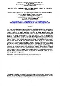
where v0(t) and vr(t) are the recorded signals at two stations separated by distance r. Equation (1) is valid for the vertical component. Corresponding and more complex formulas exist for the horizontal components of the surface waves. An example of a typical station layout is given in Figure 1a for an array with an aperture of about 100 m. The irregular shape is generally induced by natural obstacles or artificial structures (trees, streets, buildings). The end points of the vectors joining all pairs of stations are plotted in Figure 1b. For such an imperfect array, it is not possible to calculate an azimuthal average for one single distance. The solution proposed by Bettig et al. (2001) is to group pairs of stations along rings of finite thicknesses, as the pairs of gray circles drawn in Figure 1b. Equation (1) can be modified to allow the calculation of average ratios over a ring between r1 and r2. qr1 , r2 (x) ⳱
冤 冢 冣
冢 冣冥
2 c(x) xr2 xr1 r2 J1 ⳮ r1 J1 r22 ⳮ r12 x c(x) c(x)
(3)
Equation (3) has the same general shape as equation (1) and is strictly equal if r1 tends to r2. In the following, we will refer to equation (1) for the sake of simplicity. SPAC Direct Inversion The goal of the inversion is to infer the parameters of the soil structure (mainly Vs values, Vp values to a lesser extent) from the measured SPAC ratios qr1 , r2 (x). Assuming an ambient vibration wave field made in the majority of the surface waves, the SPAC curves are linked with the DC
1789
Direct Inversion of Spatial Autocorrelation Curves with the Neighborhood Algorithm
through equation (1). The DC is defined in the case of vertically heterogeneous 1D models, and its inversion is a classic problem (Herrmann, 1994). Recently, Wathelet et al. (2004) proposed to use the NA developed by Sambridge (1999) in order to investigate the parameter space in a more appropriate way. Velocity models are randomly generated by the NA core program, the corresponding phase velocities c(x) of the dispersion curves are calculated for each frequency, and the theoretical SPAC curves are obtained through equation (1) or (3). The theoretical curves are then compared to the SPAC data curves, and the fitting is characterized by a misfit value for each model. The convergence is ensured by only sampling the most promising parts of the parameter space, where the models have the lowest misfit. The random process is initiated by an arbitrary number (random seed). Two inversions with differing seeds will lead to distinct samples of the parameter space. Several independent runs (three to five) are required to test the robustness of the final results. The misfit is evaluated over all data samples. It takes into account the standard deviation derived for each SPAC sample, and it is defined in the same way as for the DC inversion (Wathelet et al., 2004):
misfit ⳱
冪兺
nR
1
nR k⳱1
nFk
nFi
兺兺
i⳱1 j⳱1
(qdij ⳮ qcij)2 rij2
Figure 1. (4)
where qdij is the SPAC ratio of data curves at frequency fj and for ring i, which is defined by all interstation distances between ri1 and ri2, qcij is the SPAC ratio of calculated curves at frequency fj and for ring i, rij is the observed variance for the sample at frequency fj and for ring i, nR is the number of rings considered, and nFi is the number of frequency samples for ring i. The SPAC inversion has basically the same limits as the DC inversion as SPAC curves are calculated from DC curves: nonuniqueness, loss of resolution with depth, and equivalence for profiles with low-velocity zones. As we plan to invert SPAC curves to obtain Vs profiles, we first address the question of the relationship between SPAC and dispersion curves. Obviously, equation (1) does not ensure a one-toone relation between the two types of curves, as the arguments for J0(x) that satisfy equation (1) can be numerous for small values of q(r, x). However, equation (1) does not imply any coupling of c(x) with the SPAC at other frequencies than x, meaning that the inversion can be made independently, frequency by frequency. Consequently, transforming SPAC curves at frequency x into their equivalent common DC is just a matter of solving a system of equations of the same form as (1) (one equation for each considered ring) and whose solutions c(x) are discrete numbers. If all the SPAC curves for the different rings are consistent with each other, there is a minimum of one solution that satisfies all apertures. From the discrete nature of the solutions and the
(a) Map of sensor locations for the array configuration used in this study. (b) Azimuth–interdistance plot: each dot represent one pair of stations. The pairs of gray circles show the limits of the chosen rings for SPAC computation.
number of rings likely to be considered, there is little chance of having two distinct solutions for c(x) that perfectly match all equations. The method is illustrated on two numerical examples: a pure synthetic test for which theoretical SPAC curves are computed and inverted, and a numerical simulation of noise seismograms for a known geometry. In both cases, uncertainties of the SPAC curves are considered. For the pure synthetic case, we derive uncertainties of the SPAC curves from Monte Carlo simulation of normally distributed deviations from the true velocity models. For the simulated ambient vibration data set, the uncertainties stem from the averaging procedure applied within the signal-processing step. In a real case, heterogeneities may add supplementary uncertainties and eventually some bias. In the following, the dispersion curves corresponding to the Vs models are computed. However, the inversion is made only on the SPAC curves.
Pure Synthetic Test The inversion method is first applied on a perfect synthetic model defined by a sedimentary layer overlying a rocky basement. Vs and Vp values inside the two layers are plotted in Figures 2a and 2b (black lines). We assume a 100m-aperture array with a quasicircular shape whose charac-
1790
M. Wathelet, D. Jongmans, and M. Ohrnberger
Figure 2. Reference model for pure and noise synthetics. (a) Vp profiles: input average model (plain line), input standard deviations (dotted lines), and generated random models ranked by their autocorrelation misfit (common gray scale). (b) Vs profiles: same legend as for Vp. (c) Dispersion curves of random models for the fundamental Rayleigh mode. (d) to (h) Autocorrelation ratios for chosen rings plotted against frequency, average, and standard deviation for all samples (dots).
teristics are given in Figure 1a. From the azimuth–distance plot of Figure 1b, we selected five distinct rings including 7 to 12 station pairs each, with an average of 10. The limits of rings were chosen to be equal to the noise synthetic case (see next example) for comparison purposes. Parametric tests show that the final results depend very little on the ring selection. We introduce uncertainties into the original model by assuming a normal distribution around the average model (black lines, Figs. 2a and 2b, with the standard deviation shown by dotted lines in the same figure). Theoretical SPAC ratios were computed for 5000 randomly generated models, keeping Poisson’s ratio constant. SPAC curves for the five rings are regularly distributed around the ones computed for the average model (black dots of figures 2d to 2h). For the inversion, a two-layer model is considered with the parameter ranges specified in Table 1. In the shallow
layer, the velocity can increase with a power-law relation, and the parameters are four (Vp, Vs /Vp, the thickness, and the Vp increase between the top and the bottom). The constant-velocity layer corresponding to the true model is a particular realization of the parametrization. The bedrock parameters are two (Vp increase and Vs /Vp). NA has been started using three independent runs with distinct random seeds, generating a total of 30,000 models. Among them about 13,500 have a misfit of less than 1 and are plotted in Figure 3. The lowest misfit is 0.03. The Vs and Vp models resulting from the SPAC inversion are plotted in Figures 3a and 3b with their misfit value. On the same figures are drawn the theoretical model of Figure 2. Most of the solutions with a misfit lower than 0.4 are able to explain in a consistent way the SPAC data given their standard deviations (Figs. 3a and 3b). In Figure 3c are plot-
1791
Direct Inversion of Spatial Autocorrelation Curves with the Neighborhood Algorithm
Table 1 Parameters for One Sediment Layer with a Power Law Variation of Vs, Overlying an Infinite Half-Space Layer
Thickness
Vp
Vs /Vp
Density
Vp Variation
Sediments Half-space
10 to 50 m —
200 to 2000 m/sec Ⳮ10 to 3000 m/sec
0.01 to 0.707 0.01 to 0.707
2 t/m3 2 t/m3
10 to 1000 m/s —
Vp, compressional velocity; Vs, shear velocity; Ⳮ, incremental velocity (the parameter is the velocity gap between the first and second layers). The power law gradient across the first layer is represented by a stack of five sub layers. The value of the parameter is the total velocity variation across the layer.
Figure 3. Inversion of the pure synthetic SPAC curves. (a) Vp profiles: true average model (black line), true standard deviations (dotted lines), and inverted models ranked by their autocorrelation misfit (common gray scale). (b) Vs profiles: same legend as for Vp. (c) Dispersion curves of generated models. (d) to (h) Autocorrelation ratios for chosen rings plotted against frequency, average, and standard deviation of data points to be fitted (dots).
ted the corresponding DCs. The Vs profile (Fig. 3b) is very well constrained from 6 to 20 meters deep. The very superficial layers (less than 6 m) are at a depth lower than onethird of the minimum wavelength (20 m), and Vs values are less constrained, resulting from the limited bandwidth at
high frequency. Below 35 m, Vs values are well constrained owing to the wide low-frequency range of the SPAC curves. In real data, this well-constrained velocity in the bedrock is usually missing because of the site high-pass filter of the Rayleigh waves below the fundamental frequency (Scher-
1792
M. Wathelet, D. Jongmans, and M. Ohrnberger
baum et al., 2003). The DCs computed for the best-fitting models compare very well with the theoretical one (Figs. 2c and 3c). The resolution is poor between 22 m and 35 m: a velocity jump at 22 m gives a misfit value equivalent to the one for a contrast at 35 m. Other inversion tests (not presented here) have shown that this lack of resolution results from the uncertainties considered on the SPAC data. However, the lowest misfit model correctly finds an interface at around 25 m depth. Usually, Vp has a low influence on the dispersion curve, and hence on the SPAC curves. Boore and Tokso¨z (1969) proved for a five-layer model that the influence of Vp on the DC is about one-tenth the influence of Vs. However, for low Poisson’s ratios, Vp has more influence. In this latter situation, the final Vs profile depends upon the correctness of the Vp profile. In classical iterative inversions (least-squares scheme), Vs /Vp, or Poisson’s ratio, is kept constant because the small influence of Vp on the SPAC curves generally leads to unrealistic velocities. For the NA inversions, the parameterization is easily adjusted to fit the physical limits of Vp and the prior information, for instance, about the superficial values of Vp. When no information is available about Vp, it is still used as a parameter with large prior intervals to prevent the alteration of the final result with unreliable assumptions. For this inversion test, we assumed that no prior information exists on Vp. As the Poisson’s ratio for the theoretical model is 0.49, the compressional-wave velocity (Vp) profile is badly recovered. Equivalent models are found for the whole prior Vp range (from 200 to 2000 m/sec in the upper layer). To test the efficiency of the SPAC inversion process, we applied the method to noise synthetics, generated with random sources generated on a 1D layered model and measured by an array of sensors.
Noise Synthetic Test
Figure 4. Simulation of ambient vibration signals. (a) Time series of vertical component for the central station of array shown in Figure 1a. (b) The smoothed Fourier spectrum for the vertical component and (c) one horizontal component.
The synthetic seismic ambient vibrations were calculated for about 60 sec using the method proposed by Hisada (1995) for the 1D average layered model described in the previous section (Figs. 2a and 2b). This method has already been successfully used for modeling noise by BonnefoyClaudet et al. (2004). A total of 333 sources points were randomly distributed both in time and space, a few meters to 600 m from the first receiver. Sources were punctual forces with delta-like functions of random amplitudes and directions, with an energy content uniformly spread from 0.5 to 8.5 Hz. The time series and the spectrum simulated at one of the receivers are plotted in Figures 4a and 4b for the vertical component. In Figure 4c, the spectrum for the north horizontal component is shown. A striking feature is the narrower range at low frequency on the vertical component, resulting from the high-pass filtering effect affecting the Rayleigh waves. The selected array geometry is the one of Figure 1a, and the SPAC curves are computed using the method proposed
by Bettig et al. (2001), with the rings shown in Figure 1b. To assess the stationarity in time of the autocorrelation ratios, we divide the 60 sec of available signals into smaller time windows. The choice of window length is crucial. In Figure 5, the SPAC curves calculated for the smaller ring (29 to 41 m) are plotted for various window lengths, counted in number of periods of the central considered frequency: 10, 25, and 50 (from light to dark gray, respectively). For the three curves, the average values are close to the true SPAC curve (thick black line) in the range 3.5 to 5.5 Hz. Below 3.5 Hz, the 10-period SPAC curve deviates from the correct function, while the two other curves (25 and 50 periods) are close to it for frequencies as low as 2.5 Hz. This discrepancy for short windows is probably due to a lack of source azimuth coverage (Asten et al., 2004), as the number of acting random sources is inversely proportional to the considered period of time. Another explanation might be that the spectral estimates are more influenced by unavoidable side ef-
Direct Inversion of Spatial Autocorrelation Curves with the Neighborhood Algorithm
1793
Figure 5. Comparison of SPAC results for different time-window lengths, average and standard deviations (ring 29 to 41 m): 10 periods (light gray), 25 periods (medium gray), and 50 periods (dark gray). The thick black line represents the theoretical SPAC curve.
fects generated by cutting signals into time windows. Also, long time-window curves are smoother than short ones and exhibit smaller standard deviations (Fig. 5). In the following discussion, the 25-period time windows are used for the SPAC curve computations. The average SPAC curves are displayed with their standard deviations in Figure 8 with gray dots and error bars, respectively. As mentioned in the Introduction, the measured SPAC curves do not always fit the shape of Bessel’s function, and the system of SPAC equations (of type 1 or 3) may have no common solution for all apertures. Feeding the inversion process with contradictory SPAC curves is likely to give an uncontrolled average solution. If the contradiction comes from a defect in the array response (e.g., too wide aperture for the considered wavelength) or in the noise content (e.g., uncorrelated noise due to a long distance between sensors for the considered frequency, or insufficient energy level at low frequency), the probability of obtaining an unrealistic solution is high. A selection of the relevant parts of the SPAC curves is thus necessary. The problem is complex, and there are no objective or commonly applicable rules. Without a prior knowledge of the soil structure, the only reliable features are the array geometry and the SPAC curves themselves. From the array geometry, some rough limits can be deduced for a correct response in terms of wavenumber (Asten and Henstridge, 1984), theoretically for the f-k processing only. The theoretical response of the array displayed in Figure 1a has been calculated and shows at least two major aliasing peaks at wavenumber 0.15 rad/m (Fig. 6, outer black circle). A rough estimate of the minimum wavenumber can be deduced from the width of the central peak of Figure 6, about 0.025 rad/m (inner black circle). On the other hand, from the SPAC curves for the different rings we can test the
Figure 6. Theoretical f-k response for array geometry of Figure 1a. Inner black circle is shown at 0.025 rad/m and the outer black circle at 0.15 rad/m. consistency of the system of equations, and discard the samples that are obviously out of the general trend. Practically, from a very large a priori value in terms of apparent velocity (e.g. from 100 to 3000 m/sec), all possible solutions c(x) of equation (1) or (3) are calculated independently for each ring. For doing so, we define the function: g(c, x) ⳱ qcalc (r, x, c) ⳮ qobs (r,x)
(5)
where x is the considered frequency band, qcalc is calculated by equation (1) or (3), and qobs is the autocorrelation ratio calculated from the simulated signals. The roots of function g(c,x) are successively bracketed by a coarse grid search starting from the lowest velocity, and then refined by an iterative scheme based on the Lagrange polynomial constructed by Neville’s method (Press et al., 1992). In a second stage, we construct a grid for each ring in the frequency– slowness domain. The grid cells are filled with 1 if at least one solution exists within the cell, and with 0 in the contrary case. All the grids are stacked, and the values in each cell give the number of consistent rings for a particular frequency–slowness pair. If the SPAC curves are consistent, the cells where the density of solutions is maximum should delineate the corresponding DC. From this plot, we determine the minimum and maximum slowness for each frequency, as well as the minimum and the maximum wavenumber for which we observe a focused DC. To reduce the subjectivity of the selection, zones where no clear consistency between
1794
M. Wathelet, D. Jongmans, and M. Ohrnberger
SPAC curves is observed are systematically rejected. Once the DC limits are set, it is straightforward to reject the contradictory data on the SPAC curves. This procedure is tested
on the preceding pure synthetic case, where no contradictory samples are present in the SPAC curves. Figure 7a shows the resulting frequency–slowness grid obtained after seeking all possible solutions. The DC can be entirely retrieved from the SPAC curves between 1 and 10 Hz. When the SPAC value is less than 0.025 (arbitrary threshold to avoid an infinite number of solutions), no solution is calculated. This is why, for high frequency, the large apertures provide no points and hence the density vanishes to one or two occurrences only. The consistency of the gray dots of Figure 8 is assessed in Figure 7b, where a zone with a high solution density clearly appears from 2.5 to 6 Hz. The maximum number of consistent rings is three, over a total of five. From the grid of Figure 7b, we delineate the lower and upper limits of the DC (thin lines) and we set the wavenumber limits (bold lines at 0.025 and 0.18 rad/m) of the denser zone, which also correspond to the f-k theoretical limits. Figure 8 shows with black dots the SPAC samples that have DC solutions within those limits. The lower wavenumber limit excludes the part of the SPAC curve where experimental points (below 2.5 Hz) do not obviously fit with a Bessel’s function (see, for instance, ring 52 to 62 m). Within the imposed limits, data correctly fit the theoretical SPAC curves (black lines), proving the relevance of the selection process. We run three inversion processes with distinct seeds and with the parameter set used in the preceding section (Table 1). The generated ensemble of models is plotted in Figure 9. Given the standard deviations, the general fit of all the SPAC curves (Fig. 9d–9h) is very good, with a minimum misfit around 0.38. In Figure 9b, we compare the true Vs profile with the inverted models: a very good resolution is achieved over the first 20 m, and a significant velocity increase is expected below. However, the Vs value in the lower part of the model is poorly resolved, mainly because of the low energy level below 3 Hz (see the Fourier spectrum in Fig. 4b). The Vp profile (Fig. 9a) shows a very wide distribution, providing little valuable information in this case. The only information is that Vp is less than 2500 m/sec in the sediment layer. The DC curves of the obtained solutions are plotted in Figure 9c, as well as the theoretical one corresponding to the true velocity model (black line). The agreement with the low-misfit solutions is globally good, particularly for frequencies greater than 3.5 Hz. We are now investigating the influence of the a priori parameterization on the results. The usual strategy is to try to find good-fitting models with the least possible number of layers, for instance, considering a power law increase of the velocity within sedimentary layers (Scherbaum et al., 2003). For our synthetic tests, we supposed a two-layer model. We test the effect of having more parameters, and the first case is a three-layer model (two sedimentary layers over the bedrock), whose characteristics are given in Table
Figure 7. Grids in the frequency–slowness domain representing the density of DC solutions. (a) DC Solutions of equation (3) for the perfect SPAC curves of Figure 2. The theoretical DC is represented by a line. (b) DC Solutions of equation (3) for brute SPAC curves of Figure 6. The chosen limits of the denser zone are delineated by thin black lines. The thick black and dotted lines represent the wavenumber limits deduced from the observations (see text).
1795
Direct Inversion of Spatial Autocorrelation Curves with the Neighborhood Algorithm
2. The number of parameters to invert are five (Vp is held constant for comparison purposes). The Vs models resulting from the inversion are shown in Figure 10a. Comparison of Figures 9b and 10a shows that lowest misfits are identical (around 0.39) and that the best models are similar, with a good resolution down to 20 m and a large uncertainty at depth. SPAC curve inversion proves to be robust and to provide a good resolution down to 20 m in this case. If we increase the number of layers (to 11) with fixed thickness (from 2 to 4 m) and if we reject low-velocity layers, we obtain the solutions of Figure 10b. Again, Figure 10b compares very well with Figures 9b and 10a. In contrast, allowing low-velocity layers in the same structure leads to the models shown in Figure 10c. Almost all models can explain the data curves in an equivalent manner and with a good misfit. In this case, the inversion is nearly uninformative about the Vs structure, owing to equivalence problems leading to a strong nonuniqueness. For earthquake engineering, the Vs profile at a given site is the major information used to assess site effects. In Figure 11, we show the SH transfer functions, which have been computed for all the models of Figure 10a. Qs has been taken as 25 for sediments and 100 for the basement. The theoretical SH response is drawn in black on the same figure for comparison. The resonance frequency (2 Hz) is globally well retrieved by the good-fitting models, as its value mainly depends on the Vs profile in the sediment layer. In contrast, the amplification at this frequency varies dramatically, resulting from the uncertainty regarding the bedrock velocity.
Real Site: Brussels, Belgium
Figure 8. (a) to (e) Brute SPAC curves calculated from the noise synthetic seismograms for the rings defined by Figure 1b, averages, and standard deviations (gray dots). Black dots are the samples that have at least one solution for the DC inside the range defined by Figure 7b. The black lines are the theoretical true SPAC curves computed from the true model.
The ambient vibrations recorded in Brussels and analyzed by Wathelet et al. (2004) with the frequency-wavenumber (f-k) method were processed with the SPAC technique described here. One of the five array geometries available for this data set (radii 25-75-130) was used for the SPAC computation. A complete analysis of the whole data set falls beyond the scope of this article. The array layout is shown in Figure 12a, and its azimuth–distance plot is shown in Figure 12b. Six rings were chosen, each one with six to nine pairs of stations. SPAC curves are computed from the measured signals (1 h and 55 min) in the same way as for the synthetic case. The results are shown in Figures 13d to 13i with gray and black dots. The consistency of those curves is tested with the grid method proposed in this article (Fig. 14). From the density plot, a common DC can be clearly identified from 1 to 3 Hz, between the thin black lines and the constant wavenumber limits (thick black lines at 0.008 and 0.056 rad/m). The SPAC samples that have no DC solution between the thin black lines and the wavenumber limits are rejected (gray dots in Figs. 13d to 13i). The observed SPAC curves might not necessarily follow the theoretical shape of the modal curves, for instance, if various modes have similar energies
1796
M. Wathelet, D. Jongmans, and M. Ohrnberger
Figure 9. Inversion of the noise synthetic SPAC curves selected in Figure 8 (black dots). (a) Vp profiles: true model (black line) and inverted models ranked by their SPAC misfit (common gray scale). (b) Vs profiles: same legend as for Vp. (c) Dispersion curves of generated models compared to the theoretical DC (black line). (d) to (h) SPAC ratios for the chosen rings plotted against frequency, average, and standard deviation of data points to be fitted (dots).
Table 2 Parameters for Two Sediment Layers with Uniform Vs, Overlying an Infinite Half-Space Layer
Thickness
Vp
Vs /Vp
Density
Vp Variation
Sediments Sediments Half-space
10 to 15 m 15 to 50 m —
1350 m/sec 1350 m/sec 2000 m/sec
0.01 to 0.707 0.01 to 0.707 0.01 to 0.707
2 t/m3 2 t/m3 2 t/m3
— — —
Vp, compressional velocity; Vs, shear velocity. See Table 1 for comments about “Vp variation” and “Ⳮ”.
in the noise wave field. This problem of a wrong mode identification may be also encountered with f-k-based methods. The selected SPAC curves (black dots) are inverted with five distinct runs of the neighborhood algorithm. The model parameterization is the same as that by Wathelet et al. (2004) (Fig. 9b, Table 2), with a sediment layer exhibiting a velocity
gradient and overlying a half-space. The generated models are plotted in Figures 13a and 13b for Vp and Vs profiles, respectively. Their corresponding SPAC curves are shown with the same gray scale in Figures 13d to 13i. The DCs calculated for all models are displayed in Figure 13c and compared with the DC obtained with the f-k method (Wath-
Direct Inversion of Spatial Autocorrelation Curves with the Neighborhood Algorithm
Figure 10. Inversion of the noise synthetic SPAC curves selected in Figure 6 (black dots) with three distinct type of parameterizations: (a) a three-layer model, (b) an 11layer model with increasing velocity profile and (c) totally free Vs profile for an 11layer model. The black line represent the theoretical Vs profile.
Figure 11.
SH response spectrum for models of Figure 10a. The inversion results are compared to the theoretical SH transfer function (thin black line).
Figure 12. (a) Map of sensor locations for the real array configuration (Brussels, Belgium). (b) Azimuth–interdistance plot: each dot represents one pair of stations. The pairs of gray circles show the limits of the rings chosen for SPAC computation.
1797
1798
M. Wathelet, D. Jongmans, and M. Ohrnberger
Figure 13.
Inversion of the real SPAC curves (black dots). (a) and (b) Vp and Vs profiles, respectively: inverted models ranked by their SPAC misfit (common gray scale). (c) Dispersion curves of generated models compared to the DC obtained with the f-k method (gray dots, from Wathelet et al., 2004). (d) to (i) SPAC ratios for the chosen rings plotted against frequency, average, and standard deviation of data points to be fitted (black dots). The gray dots are the rejected points according to the criteria defined in Figure 14.
elet et al., 2004). The curves are quite similar, and the uncertainty range of the Vs profile is almost the same as the one calculated with the f-k method.
Conclusions A direct search inversion method (the neighborhood algorithm) is applied to spatial autocorrelation (SPAC) data in order to extract Vs profiles from simulated array measurements of ambient vibrations (vertical component of the signals). In contrast to more conventional least-squares
schemes, the parameter space is deeply explored, giving a view over the posterior uncertainties of the model. Vs as a function of depth is directly obtained from the SPAC curves, through a one-step inversion processing that does not require the determination and inversion of the dispersion curve. Besides its simplicity, the advantage of this method is that the SPAC data uncertainties are fully considered during the inversion. An original contribution of this work is the definition of a methodology for assessing the valuable parts of SPAC curves to invert. The method was successfully tested on different synthetic cases (one if which is presented here),
1799
Direct Inversion of Spatial Autocorrelation Curves with the Neighborhood Algorithm
References
Figure 14. Grid in frequency–slowness domain representing the density of DC solutions of equation (3) for real SPAC curves (gray dots in Figs. 13d to 13i. The chosen limits of the denser zone are delineated by thin black lines. The thick black and dotted lines represent the wavenumber limits deduced from the observations (see text).
on synthetic random noise data, corresponding to a soft sedimentary layer overlying bedrock, and on a real case. From a practical point of view, the major limit of the method appears to be the lack of resolution at the bottom depth, resulting from the filtering effect of the soil layer on the vertical components of the signals. As with other techniques (f-k) based on the computation of the dispersion curve, the method is unable to provide reliable information below the depth of the major velocity contrast. On the other hand, the Vs profile within the soil layers is robust and well constrained if the parameterization does not allow the presence of lowvelocity zones.
Acknowledgments We thank Sylvette Bonnefoy, who agreed to share her noise seismograms, necessary for this study. This work was supported by the SESAME European project (Site EffectS assessment using Ambient Excitation, Project EVG1-CT-2000-00026). All the computer programs developed during this work are written in CⳭⳭ and will be soon available under a GPL license (www.geopsy.org for details).
Aki, K. (1957). Space and time spectra of stationary stochastic waves, with special reference to microtremors, Bull. Earthquake Res. Inst. 35, 415–456. Aki, K., and P. G. Richards (2002). Quantitative Seismology, Second Ed., University Science Books, Sausalito, California. Asten, M. W., and J. D. Henstridge (1984). Array estimators and use of microseisms for reconnaissance of sedimentary basins, Geophysics 49, 1828–1837. Asten, M. W., T. Dhu, and N. Lam (2004). Optimized array design for microtremor array studies applied to site classification; comparison of results with SCPT logs, in Proc. 13th World Conf. on Earthquake Engineering, Vancouver, 1–6 August, paper no. 1120. Bard, P.-Y. (1994). Effects of surface geology on ground motion: recent results and remaining issues, in Proc. 10th European Conf. on Earthquake Engineering, Vienna, 305–323. Bettig, B., P.-Y. Bard, F. Scherbaum, J. Riepl, F. Cotton, C. Cornou, and D. Hatzfeld (2001). Analysis of dense array noise measurements using the modified spatial auto-correlation method (SPAC). Application to the Grenoble area., Bolletino di Geofisica Teorica ed Applicata 42, 281–304. Bonnefoy-Claudet, S., C. Cornou, J. Kristek, M. Ohrnberger, M. Wathelet, P.-Y. Bard, P. Moczo, D. Fa¨h, and F. Cotton (2004). Simulation of seismic ambient noise. I. Results of H/V and array techniques on canonical models, in Proc. 13th World Conf. on Earthquake Engineering, Vancouver, 1–6 August, paper no. 2903. Boore, D. M., and M. N. Tokso¨z (1969). Rayleigh wave particle motion and crustal structure, Bull. Seism. Soc. Am. 59, 331–346. Capon, J. (1969). High-resolution frequency–wavenumber spectrum analysis, Proc. IEEE 57, 1408–1418. Chouet, B., G. De Luca, G. Milana, P. Dawson, M. Martini, and R. Scarpa (1998). Shallow velocity structure of Stromboli Volcano, Italy, derived from small-aperture array measurements of strombolian tremor, Bull. Seism. Soc. Am. 88, 653–666. Foti, S., L. Sambuelli, L. V. Socco, and C. Strobbia (2003). Experiments of joint acquisition of seismic refraction and surface wave data, Near Surface Geophys. 1, 119–129. Goldstein, P., and R. J. Archuleta (1987). Array analysis of seismic signals, Geophys. Res. Lett. 14, 13–16. Herrmann, R. B. (1994). Computer Programs in Seismology, Vol. IV, St. Louis University, St. Louis, Missouri. Hisada, Y. (1995). An efficient method for computing Green’s functions for a layered half-space with sources and receivers at close depths (part 2), Bull. Seism. Soc. Am. 85, 1080–1093. Horike, M. (1985). Inversion of phase velocity of long-period microtremors to the S-wave-velocity structure down to the basement in urbanized areas, J. Phys. Earth 33, 59–96. Jongmans, D., and D. Demanet (1993). The importance of surface waves in vibration study and the use of Rayleigh waves for determining the dynamic characteristics of soils, Eng. Geol. 34, 105–113. Lacoss, R. T., E. J. Kelly, and M. N. Tokso¨z (1969). Estimation of seismic noise structure using arrays, Geophysics 34, 21–38. Lomax, A. J., and R. Snieder (1994). Finding sets of acceptable solutions with a genetic algorithm with application to surface wave group dispersion in Europe, Geophys. Res. Lett. 21, 2617–2620. Nguyen, F., G. Van Rompaey, H. Teerlynck, M. Van Camp, D. Jongmans, and T. Camelbeeck (2004). Use of microtremor measurement for assessing site effects in Northern Belgium—interpretation of the observed intensity during the MS ⳱ 5.0 June 11, 1938 earthquake, J. Seism. 8, 41–56. Press, W. H., S. A. Teukolsky, W. T. Vetterling, and B. P. Flannery (1992). Numerical Recipes in Fortran, Second Ed., Cambridge University Press, Cambridge, U.K. Roberts, J. C., and M. W. Asten (2004). Resolving a velocity inversion at the geotechnical scale using the microtremor (passive seismic) survey method, Exploration Geophys. 35, 14–18.
1800 Sambridge, M. (1999). Geophysical inversion with a neighbourhood algorithm. I. Searching a parameter space, Geophys. J. Int. 138, 479– 494. Satoh, T., H. Kawase, and S. I. Matsushima (2001). Estimation of S-wave velocity structures in and around the Sendai Basin, Japan, using array records of microtremors, Bull. Seism. Soc. Am. 91, 206–218. Scherbaum, F., K.-G. Hinzen, and M. Ohrnberger (2003). Determination of shallow shear wave velocity profiles in the Cologne/Germany area using ambient vibrations, Geophys. J. Int. 152, 597–612. Sen, M. K., and P. L. Stoffa (1991). Nonlinear one-dimensional seismic waveform inversion using simulated annealing, Geophysics 56, 1624– 1638. Shapiro, N. (1996). Etude de l’inte´raction des ondes sismiques guide´es re´gionales avec les he´te´roge´ne´ite´s de la crouˆte, Ph.D. Thesis, Universite´ Joseph Fourier, Grenoble, France. Socco, L. V., and C. Strobbia (2004). Surface-wave method for near-surface characterization: a tutorial, Near Surface Geophys. 2, 165–185. Stokoe, K. H. II, G. J. Rix, and S. Nazarian (1989). In situ seismic testing with surface waves, in Proc. XII Intl. Conf. on Soil Mechanics and Foundation Engineering, 331–334. Tokimatsu, K. (1995). Geotechnical site characterization using surface waves, in Proc. 1st Intl. Conf. Earthquake Geotechnical Engineering, K. Ishihara (Editor), Balkema, Leiden, 1333–1368.
M. Wathelet, D. Jongmans, and M. Ohrnberger Wathelet, M., D. Jongmans, and M. Ohrnberger (2004). Surface wave inversion using a direct search algorithm and its application to ambient vibration measurements, Near Surface Geophys. 2, 211–221. LIRIGM, Universite´ Joseph Fourier BP 53 38041 Grenoble cedex 9, France
[email protected] (M.W., D.J.) GEOMAC, Universite´ de Lie`ge 1 Chemin des Chevreuils, Baˆt. B52 4000 Lie`ge, Belgium (M.W.) Institut fu¨r Geowissenschaften der Universita¨t Potsdam POB 601553 D-14415 Potsdam, Germany (M.O.)
Manuscript received 23 November 2004.