testing for spatial error autocorrelation in the

TESTING FOR SPATIAL ERROR AUTOCORRELATION IN THE PRESENCE OF ENDOGENOUS REGRESSORS

Luc Anselin Regional Research Institute and Department of Economics West Virginia University Morgantown, WV 26506-6825 [email protected]

Harry H. Kelejian Department of Economics University of Maryland College Park, Maryland 20742 [email protected]

Revised, January 1997

ABSTRACT: This paper examines the properties of Moran’s I test for spatial error autocorrelation when endogenous variables are included in the regression specification and estimation is carried out by means of instrumental variables procedures (such as two stage least squares). We formally derive the asymptotic distribution of the statistic in a general model that encompasses endogeneity due to system feedbacks as well as spatial interaction (in the form of spatially lagged dependent variables). We assess the small sample performance of the test in a series of Monte Carlo simulation experiments and compare it to a number of ad hoc approaches that have been suggested in the literature. While some of these ad hoc procedures perform surprisingly well, the new test is the only acceptable one in the presence of spatially lagged dependent variables. The test is straightforward to compute and should become part of routine specification testing of models with endogeneity that are estimated for cross-sectional data. ACKNOWLEDGMENT: We would like to thank Ingmar Prucha for helpful discussions relating to certain issues considered in this paper.

TESTING FOR SPATIAL ERROR AUTOCORRELATION IN THE PRESENCE OF ENDOGENOUS REGRESSORS

Luc Anselin and Harry H. Kelejian

1.

Introduction In empirical regional and urban economic research, many models are estimated for cross-

sectional observations on aggregate spatial units such as counties or census tracts. Such data sets are likely to exhibit a lack of independence in the form of spatial autocorrelation. This is increasingly acknowledged in applied econometric work and approached by implementing diagnostic tests for the presence of spatial autocorrelation (for reviews, see Anselin 1988a, 1988b; Anselin and Bera 1997). In the typical case, the regression model is linear, the regressors are exogenous, and the diagnostic is formulated in terms of the ordinary least squares residuals. The most popular test applied in this context is Moran’s I test for spatial autocorrelation (Moran 1950), which was generalized to regression residuals by Cliff and Ord (1972) (see also Cliff and Ord 1973, 1981). Moran’s I test is similar in structure to the familiar Durbin-Watson test for serial correlation in the time domain and shares many of its properties. In particular, it is locally best invariant (King 1981) and its exact distribution depends on the explanatory variables in the model and the dependence structure embodied in the alternative hypothesis (King 1987; Sen 1990; Tiefelsdorf and Boots 1995). Assuming normality for the errors and fixed regressors, Moran’ I is an exact test. Its distribution can be computed in small samples by means of numerical integration following the procedure suggested in Tiefelsdorf and Boots (1995). However, this is typically not done in practice. Instead, an asymptotic approximation is used that is based on the expected value and variance of the statistic under the null hypothesis of independence and normality (Cliff and Ord 1973; Sen 1976; see also Terui and Kikuchi 1994). In most cases, this approximation is quite satisfactory and the test has demonstrated superior power in several Monte Carlo simulation studies (e.g., Hordijk 1974; Bartels and Hordijk 1977; Anselin and Rey 1991; Anselin and Florax 1995). Moran’s I test is a powerful misspecification test. However, it does not provide an indication of the nature of the spatial process that causes the autocorrelation, specifically whether it is due to an error process or an omitted spatially lagged dependent variable. Other tests, based on the Lagrange Multiplier principle (e.g., Burridge 1980; Anselin 1988a, 1988c; Anselin et al. 1996)

are more appropriate in this respect, but they are asymptotic in nature and depend on the assumption of normal error terms. Also, when the misspecification is error autocorrelation, Moran’s I consistently achieves higher power in small samples than the corresponding Lagrange Multiplier test. On the other hand, LM tests are easier to implement in practice since they do not involve moment calculations as is the case for Moran’s I (see Anselin and Hudak 1992). Moran’s I and the LM tests are typically considered in a context where all explanatory variables are exogenous. In the practice of empirical regional research however, the potential endogeneity of variables in a model is increasingly acknowledged (e.g., Kelejian and Robinson 1993; Holz-Eakin 1994). Little is known about the properties of tests for spatial error autocorrelation when such endogeneity is present. The objectives of this paper are twofold. First, from a theoretical perspective, we formally derive the asymptotic distribution of Moran’s I statistic based on residuals that are obtained from an instrumental variables (IV) procedure such as two stage least squares (2SLS) in a general model that encompasses endogeneity due to system feedbacks as well as spatial interaction (spatially lagged dependent variables). In doing this, we stress the set of assumptions needed to rigorously obtain the asymptotic properties. Second, focusing on situations encountered in practice, we assess the small sample performance of the suggested test, as well as a variation which is ad hoc in nature, but has been considered in practice (e.g., Holtz-Eakin 1994). This variation boils down to the application of the moments derived in Cliff and Ord (1972) to IV residuals. We also empirically investigate the effect of endogeneity on the standard OLS-based Moran’s I and LM statistics, i.e., when the endogeneity is ignored in the estimation. Ours is the first study to address this aspect. The remainder of the paper consists of six sections. First, we outline the formal framework for the derivations in terms of the general model specification. Next we spell out the necessary assumptions. This is followed by a discussion of instrumental variable estimation and the asymptotic distribution of the statistic, both for the general model, as well as in a number of special cases. Next, the various diagnostics are evaluated empirically in a series of Monte Carlo simulation experiments. The paper closes with some concluding comments and practical recommendations. Formal proofs are relegated to the Appendix.

2.

The General Model Consider a regression model that contains both exogenous explanatory variables, as well

as endogenous variables and spatially lagged dependent variables:

—2—

*

y 1 = X 1 β + ρW N y 1∗ + Y 2 α + ε

(1)

y1 = Z1δ + ε

(2)

or, more concisely,

*

where Z 1 = ( X 1, W N y 1∗, Y 2 ) and δ′ = ( β′, ρ, α′ ) . The notation is as follows: y 1 is the N by 1 vector of observations on the dependent variable; X 1 is an N by k 1 matrix of observations on k 1 exog*

enous variables with β as the corresponding k 1 by 1 vector of parameters; W N is an N by (N + J) spatial weights matrix whose elements are known constants; y 1∗ is the (N + J) by 1 vector y 1∗ = ( y 1 ′, y 11 ′ ) , with y 11 as a J by 1 vector of observations on J values of the dependent variable that correspond to border locations; ρ is a scalar spatial autoregressive parameter; Y 2 is an N by g matrix of observations on g endogenous regressors, with α as the corresponding g by 1 parameter vector; and ε is the N by 1 vector of error terms. Throughout the paper, we will use the subscript of the spatial weights matrix to indicate its dependence on the sample size (N). *

The weights matrix W N can be partitioned to make it conformable to the partition of y 1∗ , * such that W = ( W , W˜ ) , where W is N by N and W˜ is N by J. Given this notation, equaN

N

N

N

N

tion (1) can also be written as y 1 = X 1 β + ρ ( W N y 1 + W˜N y 11 ) + Y 2 α + ε .

(3)

In practice, the border effects are typically ignored. This constitutes a special case of our general model, with J = 0 and no term of the form W˜N y 11 in equation (3). We consider border observations explicitly in order to ensure a correct model specification for each sample size N. Clearly, their omission would lead to measurement error problems (see, e.g., Griffith 1983). This is important in the derivation of the asymptotic properties and is further discussed below. The elements of y 1 and y 11 are not necessarily assumed to form a complete system. In other words, it is possible for the elements of y 11 to interact among themselves, and to interact with the elements in y 1 , as well as with other neighboring elements (not part of y 11 ). In what follows, the feedback between y 11 and y 1 is explicitly accounted for. In addition to endogeneity in the form of a spatially lagged dependent variable, our general model also involves system feedbacks contained in the matrix of endogenous variables Y 2 . This implies the existence of other unspecified equations in which the elements of Y 2 are partially determined by the elements of y 1 along with other variables. For this reason, the elements of Y 2 cannot be assumed to be unrelated to the elements of ε.

—3—

Finally, let X 2 be an N by k 2 matrix of available observations on k 2 additional exogenous variables. These are a subset of the exogenous variables appearing in the equations that determine the elements of Y 2 , but they do not appear as exogenous variables in (1). The exact specification of the equations in which these excluded exogenous variables appear does not need to be known. An illustration of the type of specification we consider here can be found in the study of regional productivity measures of Kelejian and Robinson (1997). For example, y 1i (as the i-th element in y 1 ) could represent a productivity measure for the i-th region. Then, y 1i may be explained in terms of factors specific to the i-th region, such as weather (exogenous variables), in terms of a similar productivity measure for neighboring areas, due to production externalities or technology borrowing (a spatially lagged dependent variable), and in terms of factor inputs in the i-th region that, in turn, are partially dependent upon the productivity in region i (system feedback variables).

3.

Statistical Assumptions We now proceed with a detailed outline of the set of assumptions on which the derivation

of the asymptotic properties will be based. First, we need some additional notation. In general, denote the i, j-th element, the i-th row, and the j-th column of a matrix A as, respectively, a ij , a i. , and a . j . We now consider each assumption in turn.1 Assumption 1 w Nij does not depend upon N, so that w Nij ≡ w ij ∀ N . Furthermore, w ij ≤ c w < ∞ , for all i, j = 1, . . . , N, and as N → ∞ , with c w as a finite upper bound on the magnitude of the spatial weights. This assumption requires that the elements of W N are not functions of the sample size. Essentially, this implies that the large sample analysis is conditional upon a given sequence of weights matrices. It also ensures that a sample of size N + 1 corresponds to all the units belonging to the sample of size N, plus one additional one. This is required for the asymptotics (as N → ∞ ) to work properly. This assumption would be violated if, for example, for each N the sample were to correspond to a random selection of N units from the population of all possible units. If this were the case, the sample of size N + 1 need not contain all, or even any of the units contained in the sample of size N.

1

Note that the assumptions below that directly involve a weights matrix pertain to W N . The weights matrix * W N is involved indirectly in Assumptions 8 and 9 through Z 1 from equation (2).

—4—

More importantly, Assumption 1 rules out situations in which the elements of the weights matrix are re-specified as additional observations are added to the sample. For example, this is the case when the number of neighbors for each observation is allowed to change as the sample increases in size. This would happen in the familiar row-standardized case, where each non-zero weight in the i-th row of W N equals 1 ⁄ d i , with d i as the number of neighbors for * observation i. We avoid this problem by specifying the more general W N as the weights matrix *

in (1), such that d i is the number of nonzero elements in the i-th row of W N , which will exceed the number of nonzero elements in W N when border locations are neighbors of observation i. *

However, the 1 ⁄ d i derived from the row elements in W N will not change as new observations are added to the sample (i.e., all the neighbors of observation i are already taken into account), so that Assumption 1 is not violated. Consequently, the weights structure of the model is correctly specified for each sample size. Assumption 1 may be unduly restrictive, but the technical apparatus required to treat more complex ways in which the elements of the weights matrix are affected by increasing sample size are beyond the scope of the current paper. For an in-depth treatment of the difficulties encountered in formalizing asymptotics for spatial samples, see, e.g., Cressie (1993, pp. 100–101) and Kelejian and Prucha (1996). Assumption 2 Let r N be the number of rows in W N that consist entirely of zero elements. Then, 0 ≤ r N ≤ λ 1 for all N, where λ 1 is a finite constant. This imposes a bound on the number of observations that are unconnected, or “islands,” in the sense that they have no neighbors specified in W N . Hence Assumption 2 ensures that at most λ 1 elements of y 1 are unrelated to other elements of y 1 (through W N ), even as N → ∞ . If this were not the case, a situation could arise where the sample would grow in size by adding unconnected observations. Since Moran’s I statistic is based on sums of cross products of residuals for neighboring locations (as determined by the nonzero elements in W N ), the addition of unconnected observations to the sample would only add zero to this sum. This violates a fundamental assumption of the central limit theorem needed to determine the large sample distribution of the test, since central limit theorems are based on sums of an infinite number of terms. Assumption 2 will be satisfied in most situations where there is no abrupt change in the structure of spatial dependence that is reflected in the weights matrix. For example, this will be the case for regular lattice structures.

—5—

Assumption 3 w ij ≠ 0 if and only if w ji ≠ 0 ; however, w ij need not equal w ji This requires a spatial weights matrix whose binary (boolean) form is symmetric. In other words, if unit i is viewed as neighboring unit j, then the reverse should be the case as well, although the strength of potential interaction (the value of the spatial weights) need not be identical. In practice, this assumption will be satisfied by most spatial econometric model specifications, although it precludes one-directional forms of spatial autocorrelation such as may be present in network flows. Since the latter can be treated more directly as extensions of the time series case, this is not very restrictive. Assumption 4 The sequence of spatial weights matrices W N is such that its elements w Nij satisfy the following constraints: ´

(a) w N i, i + j = 0 and w Ni. w N ( i + j ) . = 0 , for all j > λ 2 , i = 1, . . . , N – j , and N → ∞ , where λ 2 is a finite constant (b) w Nii = 0 , ∀i N

(c)

lim

N→∞

N

∑ ∑ wNij ⁄ N

= s 1 , with s 1 as a finite constant, and

i=1 j=1

(d) lim tr [ ( W N + W N ′ ) ( W N + W N ′ ) ] ⁄ N = s 2 , with s 2 as a finite constant. N→∞ The main point of Assumption 4 is that the spatial weights matrices should be such that, regardless of sample size, each element of y 1 is related to at most λ 2 other elements of y 1 . In other words, and in conjunction with Assumption 3, this implies that there are at most λ 2 nonzero elements in each row and column of W N . This can be interpreted as a bound on the extent of spatial interaction (dependence) allowed in the sample, which is needed for identification purposes (see, e.g., the discussion of mixing conditions in Anselin 1988a, Ch. 5). Furthermore, the spatial sample is assumed to grow in such a manner that units that are “sufficiently” apart from i are not neighbors of i, nor have neighbors in common (i.e., they are not second order neighbors). More precisely, this implies a form of spatial ordering of the observations, such that observations that are separated by λ 2 units (a finite constant) are neither first nor second order contiguous.

—6—

This does not pertain to the way data would be collected in practice, but is a formal mathematical (conceptual) requirement imposed to ensure that the spatial structure (the structure of W N ) does not change as the sample increases to infinity. It is satisfied by all spatial layouts in which a form of distance decay (in a proper metric, see, e.g., Weibull 1976) operates to limit the extent of interaction. As mentioned earlier, in our approach, all neighbors of i are contained in an augmented *

weights matrix W N . Assumptions 1 and 4 may be seen as unduly restrictive because they impose a given ordering of the data. However, it is important to make this ordering explicit, since without it a much more complex technical apparatus is needed to handle the way in which spatial weights matrices evolve with an increasing sample size. The assumption is not often stated in the literature, but is typically implicit. For example, in the first formal derivation of the asymptotic normality of Moran’s I by Sen (1976), the main theorem is based upon the existence of an independent and identically distributed sequence Z 1 , Z 2 , . . . (with zero mean and unit variance). However, without the assumption of a spatial ordering, the sequence should be expressed as the triangular array Z 1N , Z 2N , . . ., indicating the dependence on the sample size. Without further restrictions, this would allow Z 1N to be different from Z 1S for N ≠ S , invalidating several aspects of the relevant proofs. The second part of Assumption 4 is the standard convention that observations are not neighbors of themselves, or, that the diagonal elements of the spatial weights matrix are zero. Assumption 4(c) states that the sum of all elements in the weights matrix (the familiar normalizing constant S 0 for Moran’s I, e.g., Cliff and Ord 1981, p. 19) is at most of order N, or, stated in slightly stronger terms, that this sum deflated by N converges to a fixed constant s 1 . Since each row in W N has at most λ 2 non-zero elements that in turn are each less than c w , N

N

∑ ∑ wNij < N ( λ2 cw ) . i=1 j=1

Assumption 4(d) is similar in nature, but pertains to another familiar normalizing constant, N

N

∑ ∑ ( wNij + wNji ) i=1 j=1

N 2

= 2

N

∑ ∑ ( wNij wNji + wNij ) 2

= tr [ ( W N + W N ′ ) ( W N + W N ′ ) ]

(4)

i=1 j=1

(or, 2S 1 in the notation of Cliff and Ord 1981, p. 19). For the same reasons as before, the double

—7—

sums in (4) are also at most of order N and thus the sample size N is the proper deflator to obtain N

a constant (and finite) limit s 2 . For example, using

∑

w Nij < λ 2 c w , we see that

j=1 N

N

N

∑ ∑ wNij wNji i=1 j=1

≤

N

∑ ∑

N

w Nij

i=1 j=1

N

  2  w Nji ≤ c w w Nij  ≤ Nc w λ 2 .    i = 1 j = 1

∑ ∑

(5)

Assumption 5 The matrix ( I – ρW N ) is nonsingular at the true value of ρ , for all N. This implies that the model is complete with respect to y 1 , in the sense that equation (3) can be solved for y 1 , as –1 y 1 = ( I – ρW N ) [ X 1 β + ρ ( W˜N y 11 ) + Y 2 α + ε ] .

(6)

Assumption 6 The error terms ε i are independent and identically distributed (i.i.d.), with zero mean, 2

2

E ( ε i ) = 0 , fixed variance, E ( ε i ) = σ ε , and finite third absolute moment, E ε i

3

= µ3 .

This may be viewed as the null hypothesis, say H 0 , which implies, among other things, that the elements of the disturbance vector ε are not spatially autocorrelated. Assumption 7 The matrices of observations on the exogenous variables, X 1 and X 2 are nonstochastic, and rank ( X 1 , X 2 ) = k 1 + k 2 . In addition, consider an N by k 3 matrix X 3 whose columns are a subset of the spatially lagged exogenous variables ( W N X 1, W N X 2 ) , with k 3 ≤ k 1 + k 2 , and let X = ( X 1, X 2, X 3 ) . Then we assume that x ij ≤ c x < ∞ , with c x as a –1

finite upper bound on the elements of X, and lim N ( X′X ) = Q X , where Q X is nonN→∞ singular. This assumption implies that the analysis is conditional on the observed values of the exogenous variables in X 1 and X 2 . Furthermore, both matrices are assumed to be of full rank, and perfect multicollinearity is excluded. Also, the elements of X 1 and X 2 are assumed to be bounded, which precludes certain types of variables, such as powers or exponentials of coordinates of locations in a trend surface regression. The elements of the matrix X will serve as instru-

—8—

ments in the estimation procedure outlined in the next section. Note that if a regression contains a spatially lagged dependent variable (but no other endogenous variables), the spatial lags of the exogenous variables, W N X 1 can be used as instruments (for a rigorous treatment, see Kelejian and Robinson 1993). However, in the framework outlined here, this is not necessarily the case, since some of the excluded exogenous variables X 2 may constitute a proper instrument set. In this instance, k 3 would be zero and the instrument matrix X could simply be ( X 1, X 2 ) . However, the large sample efficiency of the IV estimator will increase with the number of instruments, i.e., with k 3 > 0 . The non-singularity of Q X is a standard assumption in a large sample framework and will typically be satisfied in practice since the elements of X are bounded and perfect multicollinearity is excluded. Assumption 8 –1

p lim ( X′X ) X′Z 1 = Π , where Π is a matrix of finite elements, with rank( Π ) = k 1 + g + 1 N→∞

This is a standard assumption needed to ensure that the parameters of the model are identified. A necessary condition for this is that k 2 + k 3 ≥ g + 1 , i.e., when there are at least as many instruments X 2 and X 3 that do not appear in equation (1) as there are regressors that are *

correlated with the error term, the endogenous variables W N y 1∗ and Y 2 . Assumption 8 also * ensures that the endogenous variables W N y 1∗ and Y 2 are at least correlated with the instruments X. Assumption 9 –1

(a)

p lim N Z 1 ′Z 1 = S 1 ,

(b)

p lim N ε′Z 1 = S 2 ,

(c)

p lim N ε′W N Z 1 = S 3 ,

N→∞

–1

N→∞

–1

N→∞

–1

(d) p lim N Z 1 ′W N Z 1 = S 4 , N→∞

where S 1 , S 2 , S 3 and S 4 are matrices of finite elements.

—9—

Assumption 9 ensures that the variables involved in the various operations needed in the estimation and in the proofs have bounded moments. Note that some of the elements of the S i matrices may be zero, for example, the elements of S 2 that pertain to the plim of the cross product of the error terms ε with the non-stochastic (Assumption 7) exogenous variables X 1 .

4.

Instrumental Variables Estimation

As is well known, the presence of the endogenous variables in Y 2 in equation (1) violates the assumption of uncorrelatedness between regressors and error term that is fundamental for the unbiasedness or consistency of the ordinary least squares estimator. Similarly, the elements *

of a spatially lagged dependent variable W N y 1∗ will be correlated with the error term ε (Anselin 1988a, p. 58). Hence, an alternative approach must be used to obtain a consistent estimator for the parameter vector δ in equation (2). In addition, the implementation of Moran’s I test for spatial error autocorrelation should not be based on residuals obtained from an inconsistent estimator such as ordinary least squares. Instead, such a test should be based upon residuals computed in terms of a consistent estimator of the model parameters. Linear models with endogenous regressors are typically estimated by means of the two stage least squares (2SLS) procedure, which is an instrumental variables method (see, e.g., Judge et al. 1985, pp. 597–599; and, for the spatial case, Anselin 1988a, pp. 81–88; Anselin 1990; Kelejian –1

and Robinson 1993). With P X = X ( X′X ) X′ as the projection matrix associated with the matrix of instruments X (defined in Assumption 7), the IV estimator for δ can be expressed as: –1 ˆ δ = ( Z 1 ′P X Z 1 ) Z 1 ′P X y 1 ,

(7)

in the notation of equation (2). As shown in a number of places (e.g., Schmidt 1976, Davidson ˆ and MacKinnon 1993), the estimator δ is consistent and asymptotically normal under a reasonable set of conditions that are satisfied by our Assumptions 1–9. More formally: N

1⁄2

D ˆ ˆ ( δ – δ ) → N [ 0, VC ( δ ) ] ,

(8)

where 2 –1 ˆ VC ( δ ) = σ ε plim N ( Z 1 ′P X Z 1 )

is the associated limiting covariance matrix.

— 10 —

(9)

The IV residuals are obtained as: ˆ εˆ = y 1 – Z 1 δ .

(10)

p ˆ Since δ is a consistent estimator for δ, or, δˆ → δ , it can be shown that when our set of asssumpˆ2 ˆ2 p 2 2 tions is satisfied, σ = ( εˆ ′εˆ ) ⁄ N is a consistent estimator for the error variance σ , or, σ → σ . ε

ε

ε

ε

Hence, approximate small sample inference for δ may be based on the normal distribution, with ˆ2 –1 ˆ . δ ≈ N δ, σ ε ( Z 1 ′P X Z 1 ) ˆ2 ˆ The consistency of δ and σ ε will be exploited in the next section to obtain the large sample properties of Moran’s I statistic based on IV residuals εˆ .

5.

Moran’s I Statistic for Residuals from Instrumental Variables Estimation Based on the IV residuals εˆ , Moran’s I statistic can be expressed as: I∗ = N ( εˆ ′W N εˆ ) ⁄ S 0 ( εˆ ′εˆ ) ,

(11)

where W N is the spatial weights matrix, and S 0 is the usual normalizing factor, N

S0 =

N

∑ ∑ wNij . i=1 j=1

ˆ Using the set of assumptions outlined in Section 3 in conjunction with the consistency of δ , we show formally in the appendix that N

1⁄2

I∗ is asymptotically normal with mean zero and finite

2

variance φ , or, 1⁄2

D

2

I ∗ → N [ 0, φ ] ,

(12) ˆ2 2 2 where φ will be discussed in more detail below. With φ replaced by a consistent estimator φ , N

an asymptotic test can be constructed such that the null hypothesis of no spatial autocorrelation may be rejected at the α level of significance if N

1⁄2

I∗ ⁄ φˆ > z α ,

(13)

where z α is the value of a standard normal variate corresponding to α. For example, taking a significance level of 5%, the null hypothesis would be rejected if the expression in (13) exceeded 1.96. Note that the exact specification of the error terms under the alternative hypothesis of spatial autocorrelation need not be known to obtain these asymptotic results. However, clearly,

— 11 —

the power of the test will depend on how well the weights matrix W N describes the pattern of spatial autocorrelation under the alternative (for a more detailed discussion of the effect of misspecified weights on the power of tests, see Florax and Rey 1995).

5.1.

Implementation of the Test in the General Case

In the general case where both endogenous variables Y 2 as well as spatially lagged * dependent variables W N y 1∗ are present in the model specification (as in equation (1)), the asymptotic variance of N

1⁄2

I∗ is shown in Appendix A to be: 2

2

2 2

φ = s 2 ⁄ ( 2s 1 ) + ( 4 ⁄ s 1 σ ε ) A ,

(14)

2

with σ ε as the error variance, s 1 and s 2 as given in Assumption 4, and –1

–1

–1

(15) A = plim [ ( N ε′W N Z 1 ) ( N ( Z 1 ′P X Z 1 ) ) ( N Z 1 ′W N ′ε ) ] . ˆ2 2 2 A consistent estimator for φ , say φ , is obtained by replacing σ ε with a consistent estimator, ˆ2 σ = ( εˆ ′εˆ ) ⁄ N , and s , s and A by their finite sample counterparts, respectively ε

1

2

N

sˆ1 =

N

∑ ∑ wNij ⁄ N , i=1 j=1

sˆ2 = ( tr [ ( W N + W N ′ ) ( W N + W N ′ ) ] ) ⁄ N , and –1 –1 –1 ˆ A = ( N εˆ ′W N Z 1 ) ( N ( Z 1 ′P X Z 1 ) ) ( N Z 1 ′W N ′εˆ ) .

Note that the first term on the right hand side of equation (15) (as well as its transpose in the third term) pertains to the probability limit of a series of cross-products of the vector of error *

terms ε with the spatial lags of the elements of Z 1 = ( X 1, W N y 1∗, Y 2 ) . Specifically, this term can be expressed as: –1

–1

–1

*

–1

plim ( N ε′W N Z 1 ) = plim ( N ε′W N X 1, N ε′W N W N y 1∗, N ε′W N Y 2 ) .

(16)

*

While W N y 1∗ and Y 2 in (16) are stochastic, X 1 is not, nor is its spatial lag, W N X 1 (Assumption 7). Furthermore, the elements of W N (of which in any row there are at most λ 2 non-zero due to Assumption 4) are bounded due to Assumption 1, and the elements of X 1 are bounded due to

— 12 —

–1

Assumption 7. Hence it can be shown that plim ( N ε′W N X 1 ) = 0 .2 This simplifies the first term in equation (16).

5.2.

Special Case: No Endogenous Regressors

When no endogenous regressors are present in the model, then Z 1 = X 1 , and, using the –1 previous result, plim ( N ε′W N Z 1 ) = 0 . Consequently, the term A in equation (14) will equal 2

2

zero and the variance φ = s 2 ⁄ ( 2s 1 ) . In this case, it follows from equation (12) that D

2

2 2 NI∗ ⁄ [ s 2 ⁄ ( 2s 1 ) ] → χ ( 1 ) ,

(17)

since the square of a standard normal variate is distributed as chi-squared with one degree of freedom. Note that equation (11) can also be written as: I∗ = [ ( εˆ ′W N εˆ ) ⁄ ( εˆ ′εˆ ) ] ⁄ ( S 0 ⁄ N ) = [ ( εˆ ′W N εˆ ) ⁄ ( εˆ ′εˆ ) ] ⁄ sˆ1 , due to Assumption 4(c), and hence, ˆ2 2 2 NI∗ ⁄ sˆ2 ⁄ 2s 1 = N [ ( εˆ ′W N εˆ ) ⁄ ( εˆ ′εˆ ) ] ⁄ ( sˆ2 ⁄ 2 )   Also, sˆ2 = tr [ ( W N + W N ′ ) ( W N + W N ′ ) ] ⁄ N = 2tr ( W N W N + W N ′W N ) ⁄ N . Therefore, the test statistic in equation (17) simplifies to ˆ2 2 ( εˆ ′W N εˆ ) ⁄ σ ε ⁄ tr ( W N W N + W N ′W N ) ,

(18)

which is Burridge’s (1980) Lagrange Multiplier (LM) statistic for spatial error autocorrelation in regression residuals (see also Anselin 1988c). In sum, the results of this special case imply that in the standard regression context the asymptotic distribution of N times the square of Moran’s I is equivalent to that of the LM-error statistic. It is important to note that this result is obtained without having to resort to a normality assumption for the error terms.

2

–1

Let ϕ = N X 1 ′W N ′ε . Then a formal proof of this property is based on the fact that E [ ϕ ] = 0 , and –1 –1 2 –1 Var [ ϕ ] = σ ε N ( N X 1 ′W N ′WN X 1 ) . Assumptions 1, 4 and 7 imply that N X 1 ′WN ′W N X 1 is bounded and thus lim Var [ ϕ ] = 0 . Hence, following Chebychev’s inequality, plim ( ϕ ) = 0 . N→∞

— 13 —

5.3.

Special Case: No Spatially Lagged Dependent Variables A special case of great interest in practice is when the model specification only contains

exogenous variables and endogenous variables Y 2 that reflect system feedbacks, or, Z 1 = ( X 1, Y 2 ) . This is the standard (i.e., non-spatial) situation in which the 2SLS procedure is used to obtain consistent parameter estimators. Then, under a reasonable set of assumptions and in the absence of spatial autocorrelation (of either spatial error or spatial lag form) in the equations that determine the endogenous variables in Y 2 , the term A in equation (14) equals zero (the precise conditions under which this holds and a proof are given in Appendix B). Consequently, under these conditions, a test for spatial error autocorrelation in models with (non-spatial) endogenous regressors can be based on the simplified form of the statistic in equations (17) or (18), which is identical in form to the usual LM-error test, but based on the residuals obtained from IV estimation (equation (10)).

6.

Monte Carlo Simulation Study We obtain an initial assessment of the size and power of the IV-based Moran’s I test from

a small number of Monte Carlo simulation experiments. We consider both the asymptotic form of the test (equations 12–16), as well as an ad hoc finite sample approximation based on the standard Cliff-Ord moments calculated in terms of IV residuals. Note that in contrast to what holds in the classic linear regression model, there is no formal basis for this approximation in the presence of endogenous regressors. We also consider the size and power of Moran’s I and the LM-Error tests computed from the residuals of an OLS estimation. These tests are clearly ad hoc, since they represent a situation in which the endogeneity of a subset of regressors is ignored. Consequently, OLS will generally be both biased and inconsistent. However, this approach may seem attractive in practice, since OLS is simple to compute relative to more complex consistent procedures and often is superior in terms of mean squared error. It is therefore important to assess the extent to which the properties of these diagnostics are affected. This aspect of our simulations extends earlier work on the effect of misspecifications on the size and power of spatial autocorrelation tests, e.g., when heteroskedasticity or non-normality are present, or when the spatial process is misspecified (see Anselin and Rey 1991; Anselin and Florax 1995; Florax and Rey 1995; Kelejian and Robinson 1995).

— 14 —

6.1.

Experimental Design The experimental design for the Monte Carlo simulations is based on a format exten-

sively used in earlier studies in the standard linear regression model (e.g., Anselin and Rey 1991; Anselin and Florax 1995). A new feature is the consideration of endogeneity. We consider two different contexts. In the first, we assess the empirical Type I errors of the tests when endogeneity is present in the form of systems feedbacks, but without a spatial lag in the model (see Section 5.3). We specify a small system of two equations, with two endogenous variables and four exogenous variables: y 1i = α 1 + β 1 x 1i + β 2 x 2i + γ 1 y 2i + ε 1i

(19)

y 2i = α 2 + β 3 x 3i + β 4 x 4i + γ 2 y 1i + ε 2i

(20)

where y 1i and y 2i are the i-th observation on the endogenous variables, x 1i , . . ., x 4i are corresponding observations for the exogenous variables, αr , γ r , r = 1, 2, and β s , s = 1, . . ., 4 are parameters, and ε 1i and ε 2i are uncorrelated error terms with mean zero and constant variance σ 2i . For the typical set of assumptions, the system (19)–(20) is overidentified, reflecting a situation often encountered in practice. For the sake of simplicity, we did not incorporate cross-equation correlation in the error terms, although this could be added in a straightforward way. In the simulations, the exogenous variables are generated as independent uniform random numbers between 0 and 1 and kept fixed in all experiments. The values for the endogenous variables are obtained by solving the reduced form of the model (19)–(20): β2 γ1 β3 γ1β4 β1 α1 + γ1α2 ε 1i + γ 1 ε 2i y 1i = ------------------------ + -------------------x 1i + -------------------x 2i + -------------------x 3i + -------------------x 4i + ------------------------1 – γ1γ2 1 – γ1 γ2 1 – γ1 γ2 1 – γ1 γ2 1 – γ1 γ2 1 – γ1 γ2

(21)

γ2 β2 γ2 β1 γ 2 ε 1i + ε 2i β3 β4 α2 + γ2 α1 y 2i = ------------------------ + -------------------x 1i + -------------------x 2i + -------------------x 3i + -------------------x 4i + ------------------------- . 1 – γ1 γ2 1 – γ1 γ2 1 – γ1 γ2 1 – γ1 γ2 1 – γ1 γ2 1 – γ1 γ2

(22)

and

Clearly, different degrees of endogeneity can be obtained by manipulating the values of the parameters and the characteristics of the error terms. In our experiments, we set all parameters equal to 1, except γ 2 , which was set equal to 0.1. This induced sufficient endogeneity to create a significant degree of simultaneity bias for the OLS estimator. For example, the bias of the OLS estimate for γ 1 was approximately −0.4 for all sample sizes (for a true value of 1.0). In comparison, the bias of the consistent IV estimator was −0.07 for samples of size N = 48 but only −0.0004

— 15 —

for samples of size N = 900. However, in terms of mean squared error (MSE), the OLS estimator was superior to the IV estimator for N = 48 and N = 81, due to its smaller sampling variance, but it was significantly inferior for the larger data sets. Specifically, for N = 900 the MSE of the OLS estimator was 0.17, compared to 0.006 for the IV estimator. Four different error distributions were considered: the standard normal, the lognormal, the uniform and the chi-squared distribution with one degree of freedom. In all cases, the generated error terms were transformed to obtain a zero mean and unit variance, using standard procedures. The second context we considered is the model in which the endogeneity consists solely of the presence of a spatially lagged dependent variable. Formally, this is expressed as y 1 = ρWy 1 + α 1 + β 1 x 1 + β 2 x 2 + ε 1

(23)

where y 1 , x 1 , x 2 and ε 1 are N by 1 vectors of values of the corresponding terms defined in (19), α 1 , β 1 and β 2 are parameters, ρ is a spatial autoregressive coefficient, and W is a known spatial weights matrix. In the simulations, we let ρ vary from 0.1 to 0.9 to assess the effect of spatial lag autocorrelation on the empirical Type I errors of test statistics. The exogenous variables are generated as before as uniform random variates, and β 1 = β 2 = 1 . The observations on the dependent variable y 1 are obtained from the usual reduced form solution –1

y 1 = ( I – ρW ) ( α 1 + β 1 x 1 + β 2 x 2 + ε 1 ) .

(24)

The power of the test statistics is compared under the alternative hypothesis of a spatial autoregressive error process ε 1 = λWε 1 + ξ 1 , with ξ 1 as an error vector whose terms are i. i. d. with mean zero and unit variance. The same four distributions were considered for ξ 1 as before: the normal, the lognormal, the uniform and the Chi-squared with one degree of freedom. The autoregressive parameter λ took values from 0.1 to 0.9. This is implemented in the simultaneous –1

system (19)–(20) by first generating ε 1 = ( I – λW ) ξ 1 , and subsequently substituting the values for ε 1 in the reduced form equations (21) and (22). Five different spatial configurations were considered: an irregular lattice structure corresponding to first order contiguity of the 48 U.S. states; and four regular lattice structures for a rook-type contiguity in square 9 by 9 (N = 81), 11 by 11 (N = 121), 30 by 30 (N = 900) and 40 by 40 (N = 1600) lattices. All spatial weights matrices were used in row-standardized form. Under the null hypothesis in the non-spatial model, 20,000 replications were generated, yielding a two standard deviation range for the empirical Type I error from 0.0469 to 0.0531 around α = 0.05 and from 0.0086 to 0.0114 around α = 0.01. For the other cases, 10,000 replica-

— 16 —

tions were used, yielding sufficient precision for our purposes (2 SD range for the empirical Type I error from 0.0456 to 0.0544 around α = 0.05 and 0.008 to 0.012 around α = 0.01). In the interest of space, only the more salient findings are listed here in some detail. A complete set of results for all cases considered is available from the authors.

6.2.

Size of the Tests in the Presence of Systems Endogeneity The first case we consider pertains to the models (19)–(20) where an endogenous systems

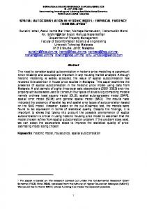
variable is contained in the specification, but no spatially lagged dependent variable. The empirical rejection frequencies under the null hypothesis of no spatial error autocorrelation for our IVError test (IV-ERR), Moran’s I test using IV residuals (I-IV), the LM test for error autocorrelation using OLS residuals (LM-OLS) and Moran’s I test applied to OLS residuals (I-OLS) are presented in Table 1 for the four error distributions and four sample sizes (the results for N = 1600 are qualitatively similar to those for N = 900). The shaded cells in the table correspond to empirical rejection frequencies that fell outside the two standard deviation (2SD) range for the nominal rejection level. Clearly, the empirical Type I errors for the IV-ERR test do not fall within a 2SD interval of the theoretical size of the test in the smallest sample size, under-rejecting the null for all four distributions. However, for the normal distribution, the test performs properly for N ≥ 81 , and for all four distributions this is the case for N = 900. Moreover, one could argue that this under-rejection is not a serious problem since the correct null is not rejected and no alternative model is estimated. The relation between the sample size and the rejection frequency of the other (ad hoc) tests is less regular. The I-IV test has the proper size for the normal distribution (for α = 0.05) in the small samples, but not for N = 900. The results are slightly better at α = 0.01. Surprisingly, Moran’s I test based on OLS residuals has the proper size in all cases with an underlying normal distribution. In other words, when normality is present and in the absence of a spatially lagged dependent variable, ignoring endogeneity in the form of system feedbacks does not seem to affect the size of Moran’s I test. The rejection frequencies of the test based on the LM-OLS statistic on the other hand only lie within the appropriate 2SD range for N ≥ 121 at α = 0.05. However, for α = 0.01 this is the case for all samples considered except N = 48. In the other cases, the null is under-rejected. The LM-OLS test also tends to be more sensitive to non-normality than the I-OLS test (again, under-rejecting the null), which confirms earlier results in the standard linear regression case (Anselin and Rey 1991). In spite of its slight discrepancies at the tail of the distribution (reflected in the under-rejection reported above), the distribution of the IV-ERR statistic under the null is remarkable close to

— 17 —

TABLE 1: Empirical Rejection Frequencies under the Null, Endogeneity Only (20,000 replications) α = 0.05

α = 0.01

Sample IV-ERR

I-IV

LM-OLS

I-OLS

IV-ERR

I-IV

LM-OLS

I-OLS

N = 48 Normal

0.0433

0.0498

0.0411

0.0482

0.0076

0.0114

0.0070

0.0103

Lognormal

0.0327

0.0404

0.0340

0.0417

0.0066

0.0095

0.0063

0.0113

Uniform

0.0451

0.0527

0.0414

0.0479

0.0079

0.0110

0.0065

0.0095

Chi-Squared

0.0324

0.0385

0.0369

0.0448

0.0066

0.0106

0.0068

0.0111

Normal

0.0499

0.0515

0.0450

0.0474

0.0103

0.0107

0.0090

0.0094

Lognormal

0.0387

0.0431

0.0324

0.0403

0.0079

0.0100

0.0054

0.0084

Uniform

0.0520

0.0555

0.0443

0.0480

0.0125

0.0134

0.0084

0.0098

Chi-Squared

0.0386

0.0414

0.0396

0.0449

0.0069

0.0085

0.0061

0.0077

Normal

0.0480

0.0508

0.0474

0.0510

0.0089

0.0098

0.0087

0.0101

Lognormal

0.0404

0.0425

0.0422

0.0464

0.0073

0.0089

0.0078

0.0093

Uniform

0.0505

0.0543

0.0498

0.0528

0.0110

0.1290

0.0099

0.0112

Chi-Squared

0.0373

0.0394

0.0435

0.0452

0.0068

0.0085

0.0077

0.0088

Normal

0.0524

0.0532

0.0499

0.0499

0.0099

0.0101

0.0106

0.0109

Lognormal

0.0485

0.0492

0.0462

0.0469

0.0100

0.0105

0.0094

0.0096

Uniform

0.0514

0.0518

0.0510

0.0524

0.0103

0.0102

0.0110

0.0116

Chi-Squared

0.0476

0.0477

0.0447

0.0461

0.0087

0.0095

0.0091

0.0093

N = 81

N = 121

N = 900

the normal, as illustrated in Figure 1 for N = 48. In the larger sample sizes, the fit to the normal distribution is almost perfect, which clearly demonstrates the asymptotic nature of the test.

6.3.

Size of the Tests in the Presence of a Spatially Lagged Dependent Variable The results in terms of the size of the various tests are strikingly different when spatial inter-

action is the source of endogeneity in the model (in the form of a spatially lagged dependent variable). The IV-ERR test is the only test that properly corrects for the complex interaction between spatial lag and spatial error dependence (see also Anselin et al. 1996), but only for very large sample sizes. As shown in Table 2 for normal errors, and apart from a few exceptions for N = 48, the test significantly over-rejects the null hypothesis for large values of ρ, and under-rejects for small val-

— 18 —

4 2 0 -2

IVERR

-4

•

•• •••• •• •••••••• • • • • • •••• •••••• ••••••• •••••••• • • • • • • ••••• ••••••• ••••••• •••••••• • • • • • • • ••••••• •••••••• •••••••••• ••••••••• • • • • • •• • • • •••••••• •••••••• ••••••••• ••••••••• • • • • • • • • • ••••••• •••••••••• ••••••••• •••••••••• • • • • • • • • •••• ••••••••• ••••••• • ••••••

-4

-2

0

2

• •

4

Quantiles of Standard Norm al

FIGURE 1: QQ-Norm Plot for IV-ERR, N = 48

TABLE 2: Rejection Frequencies under the Null Hypothesis IV-ERR Test in the Spatial Lag Model (10,000 Replications) ρ

N = 48

N = 81

N = 121

N = 900

N = 1600

0.1

0.0640

0.0251

0.0313

0.0484

0.0493

0.2

0.0742

0.0332

0.0387

0.0469

0.0464

0.3

0.0823

0.0476

0.0493

0.0505

0.0491

0.4

0.0898

0.0644

0.0650

0.0528

0.0520

0.5

0.0915

0.0878

0.0843

0.0578

0.0520

0.6

0.0887

0.1165

0.1092

0.0607

0.0551

0.7

0.0766

0.1417

0.1400

0.0638

0.0549

0.8

0.0582

0.1521

0.1694

0.0677

0.0582

0.9

0.0324

0.1248

0.1607

0.0642

0.0649

ues. Even with N = 1600, the rejection rates still exceed the 2SD bound for ρ > 0.5, although to a lesser extent. The results are qualitatively similar for non-normal errors. The performance of the ad-hoc tests is totally unacceptable in this situation, as demonstrated by the results for the I-IV test (for normal errors) in Table 3. The test significantly overrejects the null hypothesis in all samples and its performance does not improve as the sample

— 19 —

TABLE 3: Rejection Frequencies under the Null Hypothesis I-IV Test in the Spatial Lag Model (10,000 Replications) ρ

N = 48

N = 81

N = 121

0.1

0.3329

0.5031

0.5170

0.2

0.3289

0.4987

0.5215

0.3

0.3172

0.4953

0.5251

0.4

0.3030

0.4928

0.5214

0.5

0.2794

0.4788

0.5251

0.6

0.2515

0.4643

0.5212

0.7

0.2142

0.4348

0.5102

0.8

0.1689

0.3717

0.4832

0.9

0.1174

0.2760

0.3885

size increases (stabilizing around a 50% rejection rate for N = 900). The other tests are even worse in this respect. Clearly, of the tests considered the only one that appears to have reasonable empirical Type I errors in the presence of a spatially lagged dependent variable is the IV-ERR test, which applies a correction factor to Moran’s I. A comparison of the results in Table 1 to those in Tables 2 and 3 clearly illustrates the difference in the nature of the endogeneity between a system feedback variable and a spatially lagged dependent variable. As the reduced form (24) indicates, each value of the dependent variable is related to all values of the error term. This is not the case in models that contain only endogenous variables that represent system feedbacks. This suggests that the correction term A (equation 14) which is only included in the IV-ERR statistic plays a crucial role in obtaining the proper size. Also, in contrast to what is sometimes suggested in the literature, the spatially lagged dependent variable cannot be viewed as simply another endogenous variable, but the spatial nature of the endogeneity must be explicitly accounted for. Finally, from Table 2 we see that the empirical Type I errors of the IV-ERR test generally exceed the theoretical size, even in moderately sized samples such as N = 121. A rejection of the null in small samples may therefore be spurious and a further size correction of the statistic may be necessary.

6.4.

Power of the Tests The frequency with which the null hypothesis is rejected for increasing degrees of spatial

error autocorrelation is reported in Table 4, for both IV-based and OLS-based tests. In this instance, the seeming acceptability of using OLS residuals in the presence of endogenous regres-

— 20 —

TABLE 4: Power against Spatial Autoregressive Error Endogeneity Only (10,000 Replications) N = 48

N = 81

N = 121

λ IV-ERR

I-IV

IV-ERR

I-IV

IV-ERR

I-IV

0.1

0.0480

0.0805

0.0673

0.0959

0.0871

0.1164

0.2

0.0900

0.1527

0.1669

0.2258

0.2712

0.3272

0.3

0.1767

0.2682

0.3506

0.4309

0.5659

0.6231

0.4

0.3101

0.4282

0.5826

0.6630

0.8174

0.8554

0.5

0.4810

0.5928

0.7839

0.8369

0.9500

0.9625

0.6

0.6458

0.7364

0.9035

0.9271

0.9878

0.9907

0.7

0.7651

0.8297

0.9467

0.9571

0.9943

0.9947

0.8

0.8253

0.8626

0.9575

0.9643

0.9935

0.9940

0.9

0.8094

0.8489

0.9439

0.9509

0.9885

0.9891

λ

LM-OLS

I-OLS

LM-OLS

I-OLS

LM-OLS

I-OLS

0.1

0.0494

0.0773

0.0443

0.0566

0.0548

0.0696

0.2

0.0704

0.1119

0.0612

0.0879

0.1023

0.1326

0.3

0.1021

0.1640

0.1033

0.1539

0.1930

0.2384

0.4

0.1488

0.2310

0.1710

0.2390

0.3153

0.3781

0.5

0.2068

0.3127

0.2548

0.3452

0.4624

0.5318

0.6

0.2716

0.3989

0.3473

0.4451

0.5975

0.6664

0.7

0.3252

0.4692

0.4180

0.5262

0.6926

0.7590

0.8

0.3349

0.4952

0.4251

0.5442

0.7133

0.7827

0.9

0.2490

0.4038

0.2938

0.4144

0.5442

0.6332

sors has disappeared, and both IV tests show significantly superior power. The power is essentially unaffected by non-normal distributions (not reported in Table 4). Of the two, the I-IV test performs marginally better, particularly for the smaller samples and smaller values of λ, but both tests demonstrate good power against this alternative. Even in the smallest data set, the null is rejected in roughly half the cases by both tests for λ ≥ 0.5 , while for N = 121 this is already achieved for λ ≥ 0.2 and in over 95% of the cases for λ ≥ 0.5 . By contrast, the 50% mark is never reached for the OLS based tests with N = 48, and even for N = 121 the rejection frequency tops out at 78% (for the I-OLS test with λ = 0.8). In other words, there is some evidence that ignored endogeneity significantly lowers the power of OLS-based tests against spatial error autocorrelation. While in this instance an OLS estimator may still be superior to an IV estimator in terms of mean squared error, especially in

— 21 —

small samples, this attractive property does not extend to diagnostic tests based on least squares residuals.

7.

Concluding Remarks As in any simulation study, the generality of the conclusions drawn from our series of

experiments is limited by their design. We have only considered a small set of aspects related to endogeneity and the interaction between the size and power of the tests, and issues such as the number of endogenous variables, the degree of identifiability, inter-equation correlation, the choice of instruments and others that affect the properties of estimators remain to be considered. The results of the Monte Carlo simulations suggest that the asymptotic form of Moran’s I test based on IV residuals, which we derived in this paper, achieves the proper size in medium sized samples (N = 81) with normally distributed error terms, and in slightly larger samples (N = 121) for the other distributions considered. These sample sizes are typical of the number of counties in many states, or the number of census tracts in medium sized metropolitan areas, which is encouraging for empirical research. However, there is an indication that the test may underreject the null hypothesis when it is true and have less power in the presence of weak spatial error autocorrelation in the smallest sample (N = 48). On the other hand, the test seems to have good overall power, and, of those considered, is the only test that behaves properly when a spatially lagged dependent variable is included in the model. In addition, the test is easy to compute and asymptotically equivalent to the familiar Lagrange Multiplier test for spatial error autocorrelation when no spatially lagged variables are present. As a corollary, we also showed that Moran’s I test and the Lagrange Multiplier test for spatial error autocorrelation are asymptotically equivalent in the classic case when only exogenous regressors are present, without requiring the assumption of normally distributed errors. The other tests considered have been used in practice, but are ad hoc in the sense that they are not based on formal properties of the corresponding statistics. The tests based on a Moran’s I statistic formulated in terms of IV residuals has surprisingly good properties, especially when the error distribution is normal. The formal basis for these results remains to be determined. However, the attractive properties of this test hold only in the purely endogenous case. When spatially lagged dependent variables are included in the model, the test is unreliable, in the sense that the null hypothesis is rejected too frequently when no spatial error autocorrelation is present. OLS based tests, especially Moran’s I test, seem to have the proper size when the errors are normally distributed. However, ignoring endogeneity results in a significant loss in power.

— 22 —

In other words, while there is little to lose by ignoring endogeneity when no spatial error autocorrelation is present, the use of OLS-based tests in general is ill-advised since it will tend to under-reject the null when a problem is present. This is important to note, since the generally lower MSE of OLS estimators relative to IV estimators in small samples has often led to the use of OLS in practice (e.g., in the estimation of regional econometric models), even though it is inconsistent in the presence of endogenous regressors. In sum, the asymptotic properties of Moran’s I test based on IV residuals are reflected in reasonably sized samples. While the ad hoc version based on the usual mean and variance approximations also performed well in our simulations, and even achieved slightly higher power, the reason for this is not well understood. Since our test is easy to compute and is the only procedure of the ones considered that has acceptable properties in the presence of a spatially lagged dependent variable, it should be used in practice whenever instrumental variables estimation is carried out for cross-sectional data. Further work is needed in order to assess the extent to which these conclusions hold in a wider range of contexts and to understand more fully the large sample properties of the ad hoc version of the test.

— 23 —

References Anselin, L. 1988a. Spatial econometrics: Methods and models. Dordrecht: Kluwer Academic. Anselin, L. 1988b. Model validation in spatial econometrics: A review and evaluation of alternative approaches. International Regional Science Review 11: 279–316. Anselin, L. 1988c. Lagrange multiplier test diagnostics for spatial dependence and spatial heterogeneity. Geographical Analysis 20: 1–17. Anselin, L. 1990. Some robust approaches to testing and estimation in spatial econometrics. Regional Science and Urban Economics 20: 141–163. Anselin, L. and A. Bera. 1997. Spatial dependence in linear regression models with an introduction to spatial econometrics. In Handbook of Applied Economic Statistics, eds. A. Ullah and D. Giles. New York: Marcel Dekker (forthcoming). Anselin, L. and R. Florax. 1995. Small sample properties of tests for spatial dependence in regression models: Some further results. In New Directions in Spatial Econometrics, eds. L. Anselin and R. Florax, pp. 21–74. Berlin: Springer-Verlag. Anselin, L. and S. Hudak. 1992. Spatial econometrics in practice, a review of software options. Regional Science and Urban Economics 22: 509–536. Anselin, L. and S. Rey. 1991. Properties of tests for spatial dependence in linear regression models. Geographical Analysis 23: 112–31. Anselin, L., A. Bera, R. Florax and M. Yoon. 1996. Simple diagnostic tests for spatial dependence. Regional Science and Urban Economics 26: 77–104. Bartels, C.P.A. and L. Hordijk. 1977. On the power of the generalized Moran contiguity coefficient in testing for spatial autocorrelation among regression disturbances. Regional Science and Urban Economics 7: 83–101. Burridge, P. 1980. On the Cliff-Ord test for spatial autocorrelation. Journal of the Royal Statistical Society B 42: 107–108. Cliff, A. and J.K. Ord. 1972. Testing for spatial autocorrelation among regression residuals. Geographical Analysis 4: 267–284. Cliff, A. and J.K Ord. 1973. Spatial autocorrelation. London: Pion. Cliff, A. and J.K. Ord. 1981. Spatial processes: Models and applications. London: Pion. Cressie, N. 1993. Statistics for spatial data. New York: Wiley. Davidson, J. 1994. Stochastic limit theory. Oxford: Oxford University Press. Davidson, R. and J. G. MacKinnon. 1993. Estimation and inference in econometrics. New York: Oxford University Press. Florax, R. and S. Rey. 1995. The impacts of misspecified spatial interaction in linear regression models. In New Directions in Spatial Econometrics, eds. L. Anselin and R. Florax, pp. 111–135. Berlin: Springer-Verlag. Griffith, D. 1983. The boundary value problem in spatial statistical analysis. Journal of Regional Science 23: 377–387. Holtz-Eakin, D. 1994. Public-sector capital and the productivity puzzle. Review of Economics and Statistics 76: 12–21. Hordijk, L. 1974. Spatial correlation in the disturbances of a linear interregional model. Regional and Urban Economics 4: 117–140. Judge, G., W. E. Griffiths, R. Carter Hill, H. Lütkepohl and T.-C. Lee. 1985. The theory and practice of econometrics (2nd edition). New York: Wiley. Kelejian, H. H. and I. R. Prucha. 1996. A generalized moments estimator for the autoregressive parameter in a spatial model. Department of Economics, University of Maryland. Kelejian, H. H. and D. P. Robinson. 1993. A suggested method of estimation for spatial interdependent models with autocorrelated errors, and an application to a county expenditure model. Papers in Regional Science 72: 297–312.

— 24 —

Kelejian, H. H. and D. P. Robinson. 1995. A suggested test for spatial autocorrelation and/or heteroskedasticity and corresponding Monte Carlo results. Working Paper No. 95–14, Department of Economics, University of Maryland, College Park, MD. Kelejian, H. H. and D. P. Robinson. 1997. Infrastructure productivity estimation and its underlying econometric specifications. Papers in Regional Science 75 (forthcoming). King, M.L. 1981. A small sample property of the Cliff-Ord test for spatial correlation. Journal of the Royal Statistical Society B 43, 263–64. King, M.L. 1987. Testing for autocorrelation in linear regression models: A survey. In Specification Analysis in the Linear Model, eds. M. King and D. Giles, pp. 19–73. London: Routledge and Kegan Paul. Moran, P.A.P. 1950. Notes on continuous stochastic phenomena. Biometrika 37: 17–23. Schmidt, P. 1976. Econometrics. New York: Marcel Dekker. Sen, A. 1976. Large sample-size distribution of statistics used in testing for spatial autocorrelation. Geographical Analysis 9: 175–184. Sen, A. 1990. Distribution of spatial autocorrelation statistics. In Spatial statistics: past, present and future, ed. D. Griffith, pp. 257–272. Ann Arbor, MI: IMAGE. Terui, N. and M. Kikuchi. 1994. The size-adjusted critical region of Moran’s I test statistics for spatial autocorrelation and its application to geographical areas. Geographical Analysis 26: 213–227. Tiefelsdorf, M. and B. Boots. 1995. The exact distribution of Moran’s I. Environment and Planning A 27: 985–999. Weibull, J. 1976. An axiomatic approach to the measurement of accessibility. Regional Science and Urban Economics 6: 357–379.

— 25 —

APPENDIX A 1⁄2

I∗ by applying a central limit theorem and using a series of results on the limiting properties of the numerator and denominator of I∗ (equation 11). We start by considering more We derive the asymptotic distribution of N

closely both numerator and denominator of N N

1⁄2

1⁄2

I∗ ,

–1 ⁄ 2 ˆ ˆ εˆ ⁄ N ) . I∗ = ( N ε′ W N εˆ ) ⁄ sˆ1 ( ε′

(A.1)

Note that the limit of the first term in the denominator lim sˆ1 = s 1 by virtue of Assumption 4. The second element →∞ ˆ εˆ ⁄ N ) = σ 2 N(see converges to the error variance, or, plim ( ε′ Section 4). Consequently, the denominator in (A.1) conε 2

verges in probability to a non-stochastic constant s 1 σ ε . Apart from this constant, the asymptotic distribution of 1⁄2 N I∗ in (A.1) is therefore completely determined by the asymptotic distribution of the numerator term on the right hand side. We may express the 2SLS estimator δˆ (equation 7) as δˆ = δ + ∆ N ,

(A.2)

1⁄2

∆N is O p ( 1 ) in light of the limiting result in equation (8), and thus plim( ∆ N ) = 0. We can exploit this to establish a relation between the IV residuals εˆ and the error terms ε . Substituting (A.2) into equation (10) yields εˆ = y – Z ( δ + ∆ ) , or, using (2), where N

1

1

N

εˆ = ε – Z 1 ∆ N .

(A.3)

Now, we consider more closely the asymptotic properties of the numerator on the right hand side of (A.1) by substituting (A.3) into the spatial cross-products, N

–1 ⁄ 2

ˆ W εˆ = N –1 ⁄ 2 ( ε – Z ∆ )′W ( ε – Z ∆ ) ε′ N 1 N N 1 N

or, N

–1 ⁄ 2

ˆ W εˆ = N – 1 ⁄ 2 ε′W ε – 2N – 1 ⁄ 2 ( ε′W Z )∆ + N – 1 ⁄ 2 ∆ ′ ( Z ′W Z )∆ ε′ N N N 1 N N 1 N 1 N

(A.4)

After some manipulation of the powers of N, it easily follows that the second term on the right hand side of (A.4) equals – 2 ( ε′W N Z1 ⁄ N )N

1⁄2

∆ N and the third term equals N

–1 ⁄ 2

(N

1⁄2

∆ N )′ ( Z 1 ′W N Z 1 ⁄ N ) ( N

1⁄2

∆ N ) . Since N

1⁄2

∆ N is

O p ( 1 ) and bounded in probability (and thus does not vanish in the limit), and plim ( Z 1 ′W N Z 1 ⁄ N ) = S 4 (Assumption 9.d), the probability limit of the third term is zero (due to the presence of N

–1 ⁄ 2

). As a result, taking probability limits

on both sides of (A.4) yields  –1 ⁄ 2 ˆ  –1 ⁄ 2 1⁄2 –1 ⁄ 2 plim  ( N ε′ W N εˆ ) – [ ( N ε′W N ε ) – ( 2 ( ε′W N Z 1 ⁄ N )N ∆ N ) ]  = plim [ N ∆N ′ ( Z 1 ′W N Z1 )∆ N ] = 0 .  

(A.5)

Using Assumption 9.c, plim ( ε′W N Z 1 ⁄ N ) = S 3 , thus  –1 ⁄ 2 ˆ  –1 ⁄ 2 1⁄2 plim  ( N ε′ W N εˆ ) – [ ( N ε′W N ε ) – ( 2 ( ε′W N Z1 ⁄ N )N ∆ N ) ]   

.

(A.6)

 –1 ⁄ 2 ˆ  –1 ⁄ 2 1⁄2 ε′ W N εˆ ) – [ ( N ε′W N ε ) – ( 2S 3 N ∆N ) ]  = plim  ( N   The limiting properties of N

1⁄2

∆ N can be obtained more explicitly by utilizing the results in Section 4. By

substituting equation (2) for y 1 in equation (7), it follows readily that –1 ∆N = δˆ – δ = ( Z 1 ′P X Z 1 ) Z 1 ′PX ε ,

— 26 —

–1 ˆ (using the notation of Assumption 8), and thus Z ′P Z = Π ˆ ′X′XΠ ˆ , or, with Zˆ1 = P X Z 1 = X ( X′X ) X′Z 1 = XΠ 1 X 1

ˆ ′X′XΠ ˆ ) –1 Π ˆ ′X′ε , ∆N = ( Π and, thus N

1⁄2

ˆ ′ ( N –1 X′X )Π ˆ ] –1 Π ˆ ′ ( N –1 ⁄ 2 X′ε ) . ∆N = [ Π

(A.7)

Consequently, the following probability limit is obtained plim { ( N

1⁄2

–1

∆ N ) – [ Π′Q X Π ] Π′ ( N

–1 ⁄ 2

X′ε ) } = 0

(A.8)

ˆ = Π , due to Assumption 8, and plim ( N – 1 X′X ) = Q in view of Assumption 7. where plim Π X Substituting (A.8) together with the result in (A.6) into (A.5) yields  –1 ⁄ 2 ˆ  –1 ⁄ 2 –1 –1 ⁄ 2 ε′ W N εˆ ) – [ ( N ε′WN ε ) – 2S 3 [ Π′Q X Π ] Π′ ( N X′ε ) ]  = 0 plim  ( N  

(A.9)

 –1 ⁄ 2 ˆ  –1 ⁄ 2 –1 . plim  ( N ε′ WN εˆ ) – N ( ε′W N ε – 2S 3 [ Π′Q X Π ] Π′X′ε )  = 0 .  

(A.10)

or,

We simplify notation by setting –1

G ′ = – 2S3 [ Π′Q X Π ] Π′X′ ,

(A.11)

an 1 by N vector with elements g i , and Ψ = N

–1 ⁄ 2

( ε′W N ε + G ′ε ) .

(A.12)

ˆ W εˆ – Ψ ) = 0 . ε′ N

(A.13)

Then (A.10) can also be written as plim ( N

–1 ⁄ 2

Using a familiar asymptotic result, equation (A.13) implies that if we can establish the limiting distribution –1 ⁄ 2 ˆ ε′ WN εˆ . We obtain this limiting distribution by expressing Ψ

for Ψ , this will also be the limiting distribution of N

as a sum of random variables and applying the central limit theorem for m-dependent variables given in Schmidt D

2

2

(1976, p. 258). In the typical fashion, this will yield Ψ → N ( 0, σ Ψ ) , where the asymptotic variance σ Ψ must be derived from the terms that constitute Ψ . To obtain these terms, first note that N

ε′WN ε + G ′ε =

N

N

∑ ∑ εi εj wNij + ∑ gi εi , i=1 j=1

(A.14)

i=1

where g i are the elements of the vector G′ in (A.11), and the other notation is as before. Some further manipulation yields N

N

N

∑ ∑

( εi ε j w Nij ) +

∑

N

giεi =

i=1

i=1 j=1

 ∑ εi   i=1

N

∑ εj wNij j=1

 + g i  

N

=

∑ εi ( wNi . ε + g i ) i=1

or, N

Ψ≡N

–1 ⁄ 2

∑ vi i=1

— 27 —

,

(A.15)

where N

∑ εi ( wNi . ε + g i ) .

vi =

(A.16)

i=1

We now need to demonstrate that Ψ as defined in (A.16) satisfies the four conditions for the central limit theorem for m-dependent variables as described in Schmidt (1976). Condition 1: E [ v i ] = 0 This condition is satisfied since w Nii = 0 (Assumption 4.b) and thus ε i ( w Ni . ε ) in (A.16) only contains crossproducts of the form εi w Nij ε j , with i ≠ j . Since Assumption 6 specifies the error terms to be i. i. d. with zero means, E [ ε i w Nij ε j ] = 0 when i ≠ j , and also E [ ε i g i ] = 0 , therefore E [ v i ] = 0 . Condition 2: ( v 1 , . . . , v i ) is independent of ( v i + q , . . . , v N ) for all q greater than a given constant This condition is satisfied by the structure of the weights matrices imposed under Assumption 4.a (where the finite constant λ 2 plays the role of q) and the independence of the error terms in Assumption 6. Therefore, two sequences of v i that are further than λ 2 apart will have no error terms εi in common. 3

Condition 3: E [ v i ] < λ 3 , ∀i , where λ 3 is a finite constant The boundedness of the absolute third moments can be demonstrated by considering the following inequality, obtained from (A.16): 3

3

3

E [ v i ] ≤ E [ ε i ] E [ w Ni . ε + g i ] , or, after expanding the terms in the third power, 3

3

3

2

2

3

E [ v i ] ≤ E [ ε i ] E [ wNi . ε + 3 w Ni . ε g i + 3 w Ni . ε g i + g i ] .

(A.17)

Several assumptions are used to obtain the boundedness of the powers involving spatial weights and error terms in (A.17). Assumption 1 ensures that individual spatial weights are bounded by c w and Assumption 4.a. requires that there are at most λ 2 non-zero elements in each row of the spatial weights matrix. Consequently, the term w Ni . ε involves at most λ 2 cross-product terms of the form w Nij ε j whose absolute third moments are bounded by 3

3

c w E εi , which is finite in light of Assumption 6. Since the third absolute moments are bounded, all lower order absolute moments will be bounded as well. Furthermore, the elements g i are bounded because Q X , Π and S 3 are assumed to be finite matrices in Assumptions 7 through 9. This establishes bounds on the right hand side in inequality 3

(A.17) and hence the boundedness of E [ v i ] . N

Condition 4: lim Var N

–1 ⁄ 2

N→∞

∑ vi

2

= σ Ψ exists

i=1

Using (A.14),

2 σΨ

can be expressed as 2 σΨ



= lim Var N

N

N

N

–1 ⁄ 2 



εεw + gε  ∑ ∑ i j Nij ∑ i i

N→∞

i = 1

j=1

i=1

.

(A.18)



Since wNii = 0 (Assumption 4.b), the double sum over the spatial cross product terms in (A.18) can be simplified to N

N

∑ ∑ εi εj wNij i=1 j=1

N

=

N

∑ ∑

ε i ε j ( w Nij + w Nji )

(A.19)

i = 1 j = i+1

The variance of (A.19) consists of the sum of the variances of ε i ε j ( w Nij + w Nji ) and the covariances between ε i ε j ( w Nij + w Nji ) and ε r ε s ( w Nrs + w Nsr ) . Since the error terms are i. i. d. (Assumption 6), E [ ε i εj ε r εs ] = E [ ε i ]E [ ε j ]E [ ε r ]E [ ε s ] = 0 ,

— 28 —

unless two pairs of indices are equal (i = r and j = s, or i = s and j = r). Given that j > i + 1 in (A.19), all covariances are zero and the variance for each term is 2

2

2

2

2

4

2

E [ ( εi ε j ) ] ( w Nij + w Nji ) = E [ ε i ]E [ ε j ] ( wNij + w Nji ) = σ ε ( w Nij + w Nji ) , and N

Var N

–1 ⁄ 2

N

N

∑ ∑ εi εj wNij

=

–1 4 N σε

i=1 j=1

N

∑ ∑

( w Nij + w Nji )

2

(A.20)

i = 1 j= i+1

Note that the summation indices in (A.19) result in half the sum over all i, j (as in equation 4). Therefore, from equation (4) and the definition of s 2 in Assumption 4, it follows that N

lim

–1 4

N→∞

N σε

N

∑ ∑

2

4

( wNij + w Nji ) = σ ε s 2 ⁄ 2

(A.21) N

i = 1 j = i+1

Since the errors are i. i. d., the variance of the second term in (A.18) is simply N Using (A.11), it follows that

–1

∑ gi σε , or, σε G′G ⁄ N . 2 2

2

i=1 –1

–1

lim G′G ⁄ N = lim 4S 3 ( Π′Q X Π ) Π′ ( X′X ⁄ N )Π ( Π′Q X Π ) S 3 ′

N→∞

N→∞

or, since lim X′X ⁄ N = Q X due to Assumption 7, it follows that N→∞

–1

lim G′G ⁄ N = 4S 3 ( Π′Q X Π ) S 3 ′

N→∞

and thus 2

–1

2

lim σ ε G′G ⁄ N = 4σ ε S 3 ( Π′Q X Π ) S 3 ′

N→∞

(A.22)

All covariance terms between the first and second term in (A.18) are zero, since E [ ε i ε j ε r ] = 0 unless i = j, which is ruled out because w Nii = 0 . Consequently, the limit of the variance of Ψ equals the sum of (A.21) and (A.22), or 2

4

–1

2

σ Ψ = σ ε s 2 ⁄ 2 + 4σ ε S 3 ( Π′Q X Π ) S 3 ′ Since the four conditions required by Schmidt’s central limit theorem are satisfied, we can establish the limit2

ing distribution of Ψ as N ( 0, σ Ψ ) , and, due to (A.13) N

–1 ⁄ 2

D

ˆ W εˆ → N ( 0, σ 2 ) ε′ N Ψ

and thus also, N

1⁄2

D

I∗ → N [ 0, σ Ψ ⁄ ( s 1 σ ε ) ] . 2

— 29 —

2 4

APPENDIX B Z 1 = ( X 1, Y 2 ) , so that equation (15) simplifies to

For the case considered in section 5.3., –1

–1

–1

–1

plim ( N ε′W N Z 1 ) = plim ( N ε′WN X 1, N ε′WN Y 2 ) . In 5.1. and footnote 2 we showed that plim ( N ε′W N X1 ) = 0 , –1

so that for A to be zero in equation (14), we still need to demonstrate that plim ( N ε′WN Y 2 ) = 0 . For ease of exposition, we consider the case where there is only one endogenous regressor y 2 in Y 2 , so that Y 2 simplifies to a N by 1 vector. The extension to multiple endogenous variables is straightforward. The setup we described for the general model (Section 2) implied the existence of additional equations in which the endogenous system feedback variables Y 2 are determined as functions of all excluded exogenous variables X 2 . In general, each endogenous variable may therefore be expressed as a function of exogenous variables in a reduced form. Assuming such a reduced form exists and is linear, y 2 can be expressed as: y 2 = Rπ + ξ 2 ,

(B.1)

where R is a matrix with observations on the reduced variables, π is the associated vector of parameters and ξ 2 is a vector of error terms with elements ξ 2i . In line with Assumption 6 for the error terms ε , we assume that the error 2

terms ξ 2i have mean zero and a finite variance σ ξ . Furthermore, the error terms are assumed to be independently distributed over the spatial units so that E [ ξ 2i ξ 2j ] = 0 for i ≠ j . This explicitly excludes the presence of a spatially lagged dependent variable in the equation for y 2 . From (B.1) it follows that –1

–1

–1

plim ( N ε′W N y 2 ) = plim ( N ε′W N Rπ ) + plim ( N ε′W N ξ 2 ) .

(B.2)

Since Rπ is exogenous and its elements are bounded (similar to the assumptions for X), it can be shown by means of –1

the same approach as in 5.1 and footnote 2 that plim ( N ε′W N Rπ ) = 0 and thus –1

–1

plim ( N ε′W N y 2 ) = plim ( N ε′W N ξ 2 ) .

(B.3)

–1

We establish that plim ( N ε′WN ξ 2 ) = 0 in the same manner as elsewhere in this paper, by relying on Che–1

–1

bychev’s inequality together with E [ N ε′WN ξ 2 ] = 0 and lim Var [ N ε′W N ξ 2 ] = 0 . The first result readily folN→∞

lows by considering the cross products involved and using the same rationale as in Condition 1 of Appendix A N

E [ ε′W N ξ 2 ] = E

N

∑ ∑ εi ξ2j wNij

= 0,

(B.4)

i=1 j=1

since the error terms ε i and ξ 2j are independent for i ≠ j , and w Nii = 0 . The second result follows by considering the same simplification of the spatial cross-products as utilized in (A.19) together with the independence of the error terms (as in A.20), such that N

Var N

–1

N

N

∑ ∑ εi ξ2j wNij

=

–2 2 2 N σε σξ

i=1 j=1

N

∑ ∑

2

( w Nij + w Nji ) ,

i = 1 j = i+1

Also, using the definition of s 2 from Assumption 4 (analogous to the result used in A.21), it follows that N

lim

N→∞

–2 2 2 N σε σξ

N

∑ ∑

2

–1 2 2

( wNij + w Nji ) = lim N σ ε σ ξ ( s 2 ⁄ 2 ) = 0 , N→∞

i = 1 j= i+1

or, –1

lim Var [ N ε′WN ξ 2 ] = 0 .

(B.5)

N→∞

–1

The results of (B.3), (B.4) and (B.5) together with Chebychev’s inequality establish that plim ( N ε′WN y 2 ) = 0 .

— 30 —