Hindawi Publishing Corporation Mathematical Problems in Engineering Volume 2015, Article ID 609586, 17 pages http://dx.doi.org/10.1155/2015/609586
Research Article Direct Torque Control of Sensorless Induction Machine Drives: A Two-Stage Kalman Filter Approach Jinliang Zhang,1 Longyun Kang,1 Lingyu Chen,1 Boyu Yi,1 and Zhihui Xu2 1
School of Electric Power, South China University of Technology, Guangzhou, Guangdong 510640, China Sunwoda Electronic Corporation Limited, Shenzhen 518108, China
2
Correspondence should be addressed to Jinliang Zhang;
[email protected] Received 27 May 2015; Revised 27 August 2015; Accepted 27 August 2015 Academic Editor: Mohamed Djemai Copyright © 2015 Jinliang Zhang et al. This is an open access article distributed under the Creative Commons Attribution License, which permits unrestricted use, distribution, and reproduction in any medium, provided the original work is properly cited. Extended Kalman filter (EKF) has been widely applied for sensorless direct torque control (DTC) in induction machines (IMs). One key problem associated with EKF is that the estimator suffers from computational burden and numerical problems resulting from high order mathematical models. To reduce the computational cost, a two-stage extended Kalman filter (TEKF) based solution is presented for closed-loop stator flux, speed, and torque estimation of IM to achieve sensorless DTC-SVM operations in this paper. The novel observer can be similarly derived as the optimal two-stage Kalman filter (TKF) which has been proposed by several researchers. Compared to a straightforward implementation of a conventional EKF, the TEKF estimator can reduce the number of arithmetic operations. Simulation and experimental results verify the performance of the proposed TEKF estimator for DTC of IMs.
1. Introduction High performance control and estimation techniques for induction machines (IMs) have been finding more and more applications with Blaschke’s well-known field oriented control (FOC) method [1]. To improve the dynamic response of instantaneous electromagnetic torque and simplicity in control structure, one such technique for induction machine control is that the direct torque control (DTC) method can provide accurate fast torque control [2]. This method has become increasingly popular for industrial applications due to the simplified control strategy and lower parameter dependence, in comparison with the FOC methods [3, 4]. For DTC of IMs, the method requires information on the position and amplitude of the controlled stator flux for speed control applications. In the conventional approach, the stator flux is obtained utilizing a search coil or through Hall effect sensors, whilst speed sensors like incremental encoders or resolvers are used to monitor rotor velocity [2]. These unnecessarily increase hardware costs and the size of the control systems and degrade the reliability of the systems when encountering defective environments. So, sensorless
DTC strategy has become the hot issue in research and drawn many researchers and engineers’ attention. Conventional approaches to sensorless DTC of IMs employ the method of stator flux and rotor velocity estimation by using a stator voltage model [5, 6]. This method has a large error in rotor velocity estimation, particularly in the low-speed operation range. Some recent studies conducting simultaneous stator flux and rotor velocity estimation for sensorless DTC technology include model reference adaptive system (MRAS) [7], artificial neural networks (ANN) [8], sliding mode control (SMC) [9], extended Luenberger observer [10], and extended Kalman filter (EKF) [2, 11]. The model uncertainties and nonlinearities inherent to induction motors are well suited to the EKF’s stochastic nature [2]. Using this method, it is possible to make estimation of states whilst simultaneously performing identification of parameters in a short time [12–14], even taking measurement and system noises directly into system model. This explains why the EKF estimator is widely applicable in the sensorless DTC of IMs. However, the EKF may suffer numerical problems and computational burden due to the high order of the mathematical models. This has generally limited
2
Mathematical Problems in Engineering
the applicability of the EKF to real-time signal processing problems. In order to reduce the conventional EKF computational algorithm complexity, the main objective of this paper is to present a two-stage extended Kalman filter (TEKF) for stator flux, rotor speed, and electromagnetic torque estimation of a sensorless direct torque controlled IM drive. The proposed estimator is an effective implementation of EKF. Following the two-stage filtering technique as given in [15], the TEKF can be decomposed into two filters such as the modified bias free filter and the bias filter. Compared to the conventional EKF, the main advantage of the TEKF is the ability to reduce the computational complexity, whilst maintaining the same level of performance.
∙
The paper is organized as follows. In Section 2, the sensorless DTC-SVM strategy of IMs is introduced briefly. In Section 3, according to the discrete model of IM, a conventional EKF algorithm for estimating stator flux, rotor speed, and position is designed. In Section 4, TEKF are developed by the two-stage filtering approach, and its stability is analyzed. In Section 5, simulation and experimental results are discussed. Finally, a conclusion wraps up the paper.
2. Principle of Sensorless DTC-SVM As elaborated in [12], a dynamic mathematical model for an IM in the stationary (𝛼𝛽) reference frame is obtained as follows:
𝑝𝜔𝑟 𝑅𝑠 1 1 [ 𝐼𝑠𝛼 ] −𝑝𝜔𝑟 [ ∙ ] [− ( 𝜎𝐿 + 𝜎𝑇 ) 𝜎𝐿 𝑠 𝑇𝑟 𝜎𝐿 𝑠 [ ] [ 𝑠 𝑟 [ 𝐼𝑠𝛽 ] [ 𝑝𝜔 𝑅𝑠 1 1 [ ] [ 𝑝𝜔𝑟 −( + ) − 𝑟 [ ∙ ] [ 𝜎𝐿 𝑠 𝜎𝑇𝑟 𝜎𝐿 𝑠 𝜎𝐿 𝑠 𝑇𝑟 [𝜓 ] [ [ 𝑠𝛼 ] [ 0 0 0 −𝑅𝑠 [ ]=[ [ ∙ ] [ [𝜓𝑠𝛽 ] [ 0 −𝑅𝑠 0 0 [ ] [ [ ∙ ] [ [ ] [ 0 0 0 0 [ 𝜃 ] [ [ ] ∙ 0 0 0 0 [ [ 𝜔𝑟 ] where 𝐼𝑠𝛼 , 𝐼𝑠𝛽 , 𝜓𝑠𝛼 , 𝜓𝑠𝛽 , 𝑈𝑠𝛼 , and 𝑈𝑠𝛽 are the stator currents, flux linkages, and voltages in the stationary reference frame. 𝑅𝑠 and 𝐿 𝑠 are the stator winding resistance and inductance, respectively, 𝜎 is the leakage or coupling factor (where 𝜎 = 1−𝐿2𝑚 /𝐿 𝑟 𝐿 𝑠 ), 𝐿 𝑚 and 𝐿 𝑟 are the mutual inductance and rotor inductance, 𝑇𝑟 is the rotor time constant (where 𝑇𝑟 = 𝐿 𝑟 /𝑅𝑟 ), and 𝑅𝑟 is the rotor resistance. The rotor angular velocity 𝜔𝑟 is measured in mechanical radians per second, 𝜃 is the mechanical rotor position, and 𝑝 is the number of pole pairs. The behavior of an IM in DTC technique can be described in terms of space vectors by the following equations written in the stator stationary reference frame: 𝑉⃗ 𝑠 = 𝑅𝑠 𝐼⃗𝑠 +
𝑑𝜓⃗ 𝑠 , 𝑑𝑡
𝑉⃗ 𝑟 = 𝑅𝑟 𝐼⃗𝑟 + 𝑗𝜔𝑟 𝜓⃗ 𝑟 +
𝑑𝜓⃗ 𝑟 = 0, 𝑑𝑡
𝜓⃗ 𝑠 = 𝐿 𝑠 𝐼⃗𝑠 + 𝐿 𝑚 𝐼⃗𝑟 ,
(2)
𝜓⃗ 𝑟 = 𝐿 𝑠 𝐼⃗𝑟 + 𝐿 𝑚 𝐼⃗𝑠 , 𝐿 3 𝜓⃗ 𝜓⃗ sin 𝛿, 𝑇𝑒 = 𝑝 2 𝑚 2 𝐿 𝑚 − 𝐿 𝑠𝐿 𝑟 𝑠 𝑟 where 𝛿 is known as load angle which is the angle between rotor flux 𝜓⃗ 𝑟 and stator flux 𝜓⃗ 𝑠 . |𝜓⃗ 𝑠 | and |𝜓⃗ 𝑟 | are amplitudes of 𝜓⃗ 𝑠 and 𝜓⃗ 𝑟 , respectively. From (2), it can be seen that the instantaneous electromagnetic torque control of IMs in DTC
1 0 0] 𝐼𝑠𝛼 0 ] 𝜎𝐿 ][ ] [ 𝑠 [ ][𝐼 ] [ 1 ] ] ] 𝑠𝛽 ] ] [ 0 0 0] [ ] [ [ 𝜎𝐿 𝑠 ] ] [𝜓𝑠𝛼 ] [ ] 𝑈 ] 0 ] [ 𝑠𝛼 ] , ]+[ 1 0 0] [ ] 𝑈 ] [ ][ [𝜓𝑠𝛽 ] [ 0 𝑠𝛽 1 ] ] ] [ 0 0] ][ ] ] [ [ ][ 𝜃 ] [ 0 ] 0 1] ] [ 0 ] 𝜔𝑟 ] [ 0 0 0 0] ] [
(1)
is determined by changing the values of load angle 𝛿 while 𝜓⃗ 𝑠 and 𝜓⃗ 𝑟 maintain the constant amplitude. Accelerating the stator flux, with respect to the rotor flux vector, will increase the electromagnetic torque, and decelerating the same vector will decrease the electromagnetic torque [16]. The basic idea of DTC technique of IM is to control and acquire accurate knowledge on the stator flux and electromagnetic torque to achieve high dynamic performance. DTC technique involves stator flux, electromagnetic torque estimators, hysteresis controllers, and a simple switching logic (switching tables) in order to reduce the electromagnetic torque and stator flux errors rapidly [17, 18]. Due to the fact that the universal voltage inverter has only eight available basic space vectors and only one voltage space vector is maintained for the whole duration of the control period, the conventional approach causes high ripples in stator flux, current, and electromagnetic torque, accompanied by acoustical noise. To reduce the ripples of the stator flux linkage current and electromagnetic torque in IM drives, a modified DTC using Space Vector Modulation (SVM) method called DTCSVM is proposed in this paper. The main difference between conventional DTC and DTC-SVM is that DTC-SVM has a SVM model and two PI controllers instead of switching table and hysteresis controllers [19, 20]. The system structure of DTC-SVM can be built and shown in Figure 1. This system operates at constant stator flux (below rated speed). From Figure 1, the reference torque 𝑇𝑒∗ is generated from regulated speed proportional integral (PI); Δ𝑇𝑒 is the torque error ̂ 𝑒. between the reference torque 𝑇𝑒∗ and estimated torque 𝑇
Mathematical Problems in Engineering
3 ̂ s𝛼 𝜓
𝜔∗r
+ −
PI
Te∗ +
ΔTe
𝜃s∗
Δ𝛿 +
PI
+
−
𝜓∗s𝛼 −
P
∗ Vs𝛼
+
A
Stator
∗ 𝜓s𝛽
R
|𝜓 ∗s |
Δ𝜓∗s𝛼
C
∗ Vs𝛽
cal.
+ −
B
SVM
voltage
∗ Δ𝜓s𝛽
Pulses
𝜃̂s ̂e T
̂r 𝜔
Arctan
̂ s𝛼 𝜓 ̂ s𝛽 𝜓
̂ s𝛽 𝜓
̂ s𝛼 𝜓 ̂ s𝛽 𝜓
Rs Is𝛼
Rs Is𝛽
Stator flux, speed, and
Is𝛼 Is𝛽
torque estimator
𝜔r
IU IW
abc
IV
𝛼𝛽
Incremental encoder
IM
Figure 1: System diagram of the DTC-SVM scheme.
In order to compensate this error, the angle of stator flux vector must be increased from 𝜃𝑠 to 𝜃𝑠 + Δ𝛿 as shown in Figure 2, where 𝜃𝑠 is the phase angle of stator flux vector that can be obtained by the flux estimator and Δ𝛿 is the increment of stator flux in the next sampling time. Therefore, the required reference stator flux in polar form is given by ∗ 𝜓⃗ 𝑠 = |𝜓⃗ 𝑠 |∠𝜃𝑠∗ . ∗ Define the stator flux deviations between 𝜓⃗ 𝑠 and 𝜓⃗ 𝑠 as Δ𝜓⃗ 𝑠 ; then ∗ ̂ 𝑠𝛼 , Δ𝜓𝑠𝛼 = 𝜓⃗ 𝑠 cos (𝜃𝑠∗ ) − 𝜓 (3) ∗ ̂ 𝑠𝛽 , Δ𝜓𝑠𝛽 = 𝜓⃗ 𝑠 sin (𝜃𝑠∗ ) − 𝜓 where Δ𝜓⃗ 𝑠𝛽 and Δ𝜓⃗ 𝑠𝛼 are the stationary axis components of ̂ 𝑠𝛼 and 𝜓 ̂ 𝑠𝛽 are the stator flux components stator flux Δ𝜓⃗ 𝑠 and 𝜓 estimation. In order to make up for stator flux deviations Δ𝜓𝑠𝛼 ∗ ∗ and Δ𝜓𝑠𝛽 , the reference stator voltages 𝑈𝑠𝛼 and 𝑈𝑠𝛽 should be applied on the IM which can be expressed by ∗ 𝑈𝑠𝛼 = 𝑅𝑠 𝐼𝑠𝛼 + ∗ 𝑈𝑠𝛽
= 𝑅𝑠 𝐼𝑠𝛽 +
Δ𝜓𝑠𝛼 , 𝑇𝑠 Δ𝜓𝑠𝛽 𝑇𝑠
(4)
.
Substituting (3) into (4), (5) can be acquired: ∗ ̂ 𝑠𝛼 ) (𝜓⃗ 𝑠 cos (𝜃𝑠∗ ) − 𝜓 ∗ 𝑈𝑠𝛼 = 𝑅𝑠 𝐼𝑠𝛼 + , 𝑇𝑠 ∗ ̂ 𝑠𝛽 ) (𝜓⃗ 𝑠 sin (𝜃𝑠∗ ) − 𝜓 ∗ . 𝑈𝑠𝛽 = 𝑅𝑠 𝐼𝑠𝛽 + 𝑇𝑠
𝜓s∗
𝛽
Δ𝜓s 𝜓s
𝜓r 𝜃∗s
Δ𝛿 𝛿 𝜃r
𝜃s
𝛼
Figure 2: Control of stator flux linkage.
∗ Based on the reference stator voltage components 𝑈𝑠𝛼 ∗ and 𝑈𝑠𝛽 , the drive signal for inverter IGBTs can be obtained through SVM module. Then, both the electromagnetic torque and the magnitude of stator flux are under control, thereby generating the reference stator voltage components.
3. Conventional EKF Theory (5)
By choosing the system state vector and estimated parameter 𝑇 𝑇 vector as 𝑋(𝑡) = [𝐼𝑠𝛼 𝐼𝑠𝛽 𝜓𝑠𝛼 𝜓𝑠𝛽 ] and 𝑟(𝑡) = [𝜃 𝜔𝑟 ] , 𝑇 respectively, 𝑢(𝑡) = [𝑈𝑠𝛼 𝑈𝑠𝛽 ] as the input vector, and
4
Mathematical Problems in Engineering 𝑇
𝑌(𝑡) = [𝐼𝑠𝛼 𝐼𝑠𝛽 ] as the output vector, the IM model is described by the general nonlinear state space model:
The solution of nonhomogenous state equations (6) satisfying the initial condition 𝑋(𝑡)|𝑡=𝑡0 = 𝑋(𝑡0 ) is
∙
𝑋 (𝑡) = 𝐴 (𝑡) 𝑋 (𝑡) + 𝐵 (𝑡) 𝑢 (𝑡) + 𝐷 (𝑡) 𝑟 (𝑡) , ∙
𝑡
𝑋 (𝑡) = 𝑒𝐴(𝑡−𝑡0 ) 𝑋 (𝑡0 ) + ∫ 𝑒𝐴(𝑡−𝜏) 𝐵𝑢 (𝜏) 𝑑𝜏.
(6)
𝑟 (𝑡) = 𝐺 (𝑡) 𝑟 (𝑡) , 𝑌 (𝑡) = 𝐶 (𝑡) 𝑋 (𝑡)
𝑡0
(9)
Integrating from 𝑡0 = 𝑘𝑇𝑠 to 𝑡 = (𝑘 + 1)𝑇𝑠 , we can obtain that
with 𝐴 (𝑡)
𝑋 ((𝑘 + 1) 𝑇𝑠 ) = 𝑒𝐴𝑇𝑠 𝑋 (𝑘𝑇𝑠 )
𝑝𝜔𝑟 𝑅𝑠 1 1 −𝑝𝜔𝑟 [− ( 𝜎𝐿 + 𝜎𝑇 ) 𝜎𝐿 𝑠 𝑇𝑟 𝜎𝐿 𝑠 ] ] [ 𝑠 𝑟 [ 𝑝𝜔𝑟 𝑅𝑠 1 ] 1 ] [ 𝑝𝜔𝑟 −( + ) − ], =[ [ 𝜎𝐿 𝜎𝑇 𝜎𝐿 𝜎𝐿 𝑇 𝑠 𝑟 𝑠 𝑠 𝑟] ] [ [ −𝑅𝑠 0 0 0 ] ] [ 0 −𝑅 0 0 𝑠 ] [ 𝑇 1 0 1 0] [ 𝜎𝐿 𝑠 ] , 𝐵 (𝑡) = [ ] [ 1 0 1 0 𝜎𝐿 𝑠 ] [
+∫
𝑘𝑇
𝐴 𝑘 = 𝑒𝐴𝑇𝑠 ,
(7)
𝐵𝑘 = 𝐴−1 (𝑒𝐴𝑇𝑠 − 𝐼) 𝐵.
0 0
(10)
(11)
In the same way,
1 0 0 0 ], 𝐶 (𝑡) = [ 0 1 0 0 𝐺 (𝑡) = [
𝑒𝐴((𝑘+1)𝑇𝑠 −𝜏) 𝐵 𝑑𝜏𝑢 (𝑘𝑇𝑠 ) .
The above equations lead to
𝐷 (𝑡) = 0,
0 1
(𝑘+1)𝑇𝑠
𝐺𝑘 = 𝑒𝐺𝑇𝑠 .
(12)
].
Remark 1. Matrices 𝐶(𝑡) and 𝐺(𝑡) are not affected by uncertainties.
Tolerating a small discretization error, a first-order Taylor series expansion of the matrix exponential is used: 𝐴 𝑘 = 𝑒𝐴𝑇𝑠 ≈ 𝐴𝑇𝑠 + 𝐼,
Remark 2. Matrix 𝐴(𝑡) is time-varying because it depends on the rotor speed 𝜔𝑟 . For digital implementation of estimator on a microcontroller, a discrete time mathematical model of IMs is required. These equations can be obtained from (6):
𝐺𝑘 = 𝑒𝐺𝑇𝑠 ≈ 𝐺𝑇𝑠 + 𝐼, 𝐵𝑘 = 𝐴−1 (𝑒𝐴𝑇𝑠 − 𝐼) 𝐵 ≈ 𝑇𝑠 𝐵,
𝑋𝑘+1 = 𝐴 𝑘 𝑋𝑘 + 𝐵𝑘 𝑢𝑘 + 𝐷𝑘 𝑟𝑘 , 𝑟𝑘+1 = 𝐺𝑘 𝑟𝑘 ,
𝐷𝑘 = 0
(8)
𝑌𝑘 = 𝐶𝑘 𝑋𝑘 .
with
𝑝𝜔𝑟 𝑇𝑠 𝑇𝑠 𝑇𝑠 𝑅𝑠 𝑇𝑠 −𝑝𝜔𝑟 𝑇𝑠 [− ( 𝜎𝐿 + 𝜎𝑇 ) + 1 𝜎𝐿 𝑇 𝜎𝐿 𝑠 ] 𝑠 𝑟 𝑠 𝑟 [ ] [ ] 𝑝𝜔𝑟 𝑇𝑠 𝑇𝑠 ] 𝑅𝑠 𝑇𝑠 𝑇𝑠 [ [ ], 𝑝𝜔 𝑇 − ( + ) + 1 − 𝐴𝑘 = [ 𝑟 𝑠 𝜎𝐿 𝑠 𝜎𝑇𝑟 𝜎𝐿 𝑠 𝜎𝐿 𝑠 𝑇𝑟 ] [ ] [ −𝑅𝑠 𝑇𝑠 0 1 0 ] [ ] 0 −𝑅 𝑇 0 1 𝑠 𝑠 [ ] G𝑘 = [
1 𝑇𝑠 0 1
],
(13)
Mathematical Problems in Engineering
5
𝑇 𝑇𝑠 0 𝑇 0 𝑠 ] [ 𝜎𝐿 𝑠 ] , 𝐵𝑘 = [ ] [ 𝑇𝑠 0 𝑇𝑠 0 𝜎𝐿 𝑠 ] [
𝐶𝑘 = [ 𝐷𝑘 = [
1 0 0 0 0 1 0 0
],
0 0 ]. 0 0 (14)
Based on discretized IM model, a conventional EKF estimator is designed for estimation of stator flux, current, electromagnetic torque, and rotor speed of IM for sensorless DTC-SVM operations. Treating 𝑋𝑘 as the full order state and 𝑟𝑘 as the augmented system state, the state vector is chosen to 𝑇 𝑇 𝑇 be 𝑋𝑘𝑎 = [𝑋𝑘 𝑟𝑘 ] . 𝑢𝑘 = [𝑈𝑠𝛼 𝑈𝑠𝛽 ] and 𝑌𝑘 = [𝐼𝑠𝛼 𝐼𝑠𝛽 ] are chosen as input and output vectors because these quantities can be easily obtained from measurements of stator currents and voltage construction using DC link voltage and switching status. Considering the parameter errors and noise of system, the discrete time state space model of IMs in the stationary (𝛼𝛽) reference frame is described by
The initial conditions are assumed to be Gaussian random variables 𝑋0 and 𝑟0 that are defined as follows:
𝑎 = 𝐴𝑘 𝑋𝑘𝑎 + 𝐵𝑘 𝑢𝑘 + 𝑤𝑘 , 𝑋𝑘+1
The overall structure of the EKF is well-known by employing a two-step prediction and correction algorithm [13]. Hence, the application of EKF filter to the state space model of IM (15) is described by
𝑌𝑘+1 = 𝐶𝑘 𝑋𝑘𝑎 + V𝑘
(15)
𝑇
𝐸 ((𝑋0 − 𝑋0∗ ) (𝑋0 − 𝑋0∗ ) ) = 𝑃0𝑥 , 𝐸 (𝑋0 ) = 𝑋0∗ , 𝐸 (𝑟0 ) = 𝑟0∗ 𝑇
𝐸 ((𝑟0 − 𝑟0∗ ) (𝑟0 − 𝑟0∗ ) ) = 𝑃0𝑟 , 𝑇
𝐸 ((𝑋0 − 𝑋0∗ ) (𝑟0 − 𝑟0∗ ) ) = 𝑃0𝑥𝑟 .
with 𝐴𝑘 = [ 𝐵𝑘 = [ 𝐶𝑘 = [ 𝑤𝑘 = [
𝐴 𝑘 𝐷𝑘 0 𝐺𝑘 𝐵𝑘 0
0
𝑎 𝑎 = 𝐴𝑘−1 𝑋𝑘−1|𝑘−1 + 𝐵𝑘−1 𝑢𝑘−1 , 𝑋𝑘|𝑘−1
],
𝑇
𝑇
𝑇
𝑇
−1
𝑃𝑘|𝑘 = 𝑃𝑘|𝑘−1 − 𝐾𝑘 𝐻𝑘 𝑃𝑘|𝑘−1 ,
(16)
(21) (22)
𝑎 𝛼 𝑎 𝑋𝑘|𝑘 = 𝑋𝑘|𝑘−1 + 𝐾𝑘 (𝑌𝑘 − 𝐶𝑘 𝑋𝑘|𝑘−1 )
] , with
𝑤𝑘𝑥
]. 𝑤𝑘𝑟
𝑄𝑘𝑥 0 0 ] [ ] = [ 0 𝑄𝑘𝑟 0 ] ] 𝛿𝑘𝑗 , ] ] [ 0 0 𝑅𝑘 ]
𝑇
(20)
𝐾𝑘 = 𝑃𝑘|𝑘−1 𝐻𝑘 (𝐻𝑘 𝑃𝑘|𝑘−1 𝐻𝑘 + 𝑅) ,
𝐹𝑘−1 = [
The system noise 𝑤𝑘 and measurement noise V𝑘 are white Gaussian sequence with zero-mean and following covariance matrices: 𝑤𝑗𝑥 𝑤𝑘𝑥 [[ 𝑟 ] [ 𝑟 ] [ ] 𝐸[ [[ 𝑤𝑘 ] [ 𝑤𝑗 ] [[ V𝑘 ] [ V𝑗 ]
(19)
𝑃𝑘|𝑘−1 = 𝐹𝑘−1 𝑃𝑘−1|𝑘−1 𝐹𝑘−1 + 𝑄𝑘−1 ,
],
𝐶𝑘
(18)
(17)
where 𝑄𝑘𝑥 > 0, 𝑄𝑘𝑟 > 0, 𝑅𝑘 > 0, and 𝛿𝑘𝑗 is the Kronecker delta. The initial states 𝑋0 and 𝑟0 are assumed to be uncorrelated with the zero-mean noises 𝑤𝑘𝑥 , 𝑤𝑘𝑟 , and V𝑘 .
𝑄 (⋅) = [
𝐹𝑘−1 𝐸𝑘−1 0
𝐺𝑘−1
],
𝑄𝑥 (⋅)
0
0
𝑟
𝑄 (⋅)
],
𝐹𝑘−1 =
𝜕 (𝐴 𝑋 + 𝐵𝑘−1 𝑢𝑘−1 + 𝐷𝑘−1 𝑟𝑘−1 ) = 𝐴 𝑘 , 𝜕𝑋 𝑘−1 𝑘−1
𝐸𝑘−1 =
𝜕 (𝐴 𝑋 + 𝐵𝑘−1 𝑢𝑘−1 + 𝐷𝑘−1 𝑟𝑘−1 ) 𝜕𝑟 𝑘−1 𝑘−1
=[
0
0 0 0
𝑝1 𝑝2 0 0
𝑇
] ,
(23)
6
Mathematical Problems in Engineering 𝑝1 = (−𝑝𝑖𝑠𝑏[𝑘−1|𝑘−1] + 𝑝2 = (𝑝𝑖𝑠𝛼[𝑘−1|𝑘−1] − 1
2
𝐻𝑘 = [𝐻𝑘 𝐻𝑘 ] =
𝑝 𝜓 )𝑇 , 𝜎𝐿 𝑠 𝑠𝛽[𝑘−1|𝑘−1] 𝑠
The main advantage of using the 𝑇(𝑈𝑘 ) transformation is that the inverse transformation 𝑇−1 (𝑈𝑘 ) = 𝑇(−𝑈𝑘 ) involves only a change of sign. Two blending matrices 𝑈𝑘 and 𝑉𝑘 𝑥𝑟 𝑟 𝑥𝑟 𝑟 −1 are defined by 𝑈𝑘 = 𝑃𝑘|𝑘−1 (𝑃𝑘|𝑘−1 )−1 and 𝑉𝑘 = 𝑃𝑘|𝑘 (𝑃𝑘|𝑘 ) , respectively. Using characteristic of 𝑇(𝑈𝑘 ), (25) become
𝑝 𝜓 )𝑇 , 𝜎𝐿 𝑠 𝑠𝛼[𝑘−1|𝑘−1] 𝑠
𝜕 (𝐶 𝑋𝑎 ) , 𝜕𝑋𝑎 𝑘
𝑎
𝑎 𝑋𝑘|𝑘−1 = 𝑇 (−𝑈𝑘 ) 𝑋𝑘|𝑘−1 ,
1
𝐻𝑘 = 𝐶𝑘 ,
𝑇
𝑃𝑘|𝑘−1 = 𝑇 (−𝑈𝑘 ) 𝑃𝑘|𝑘−1 𝑇 (−𝑈𝑘 ) ,
2
𝐻𝑘 = 0,
𝐾𝑘 = 𝑇 (−𝑉𝑘 ) 𝐾𝑘 , 𝑥
𝑥𝑟
𝑃 (⋅) 𝑃 (⋅) 𝑃 (⋅) = [ 𝑥𝑟 ]. 𝑇 (𝑃 (⋅)) 𝑃𝑟 (⋅)
𝑇
𝑃𝑘|𝑘 = 𝑇 (−𝑉𝑘 ) 𝑃𝑘|𝑘 𝑇 (−𝑉𝑘 ) , 𝑎
𝑎 𝑋𝑘|𝑘 = 𝑇 (−𝑉𝑘 ) 𝑋𝑘|𝑘 .
(24)
And the following relationships are obtained from (25):
4. The Two-Stage Extended Kalman Filter 4.1. The TEKF Algorithm. As mentioned in conventional EKF estimator previously, the memory and computational costs increase with the augmented state dimension. Considering sampling time is very small, only high performance microcontroller can qualify for this work. Hence, the conventional EKF algorithm may be impractical to implement. The extra computation of 𝑃𝑥𝑟 (⋅) terms leads to this computational complexity. Therefore we can reduce the computational complexity from application point of view if the 𝑃𝑥𝑟 (⋅) terms can be eliminated. In this section, a two-stage extended Kalman filter without explicitly calculating 𝑃𝑥𝑟 (⋅) terms is discussed. Following the same approach as given in [15], the TEKF is decomposed into two filters such as the modified bias free filter and the bias filter by applying the following two-stage 𝑈-𝑉 transformation: 𝑎
𝑎 = 𝑇 (𝑈𝑘 ) 𝑋𝑘|𝑘−1 , 𝑋𝑘|𝑘−1
𝐾𝑘 = 𝑇 (𝑉𝑘 ) 𝐾𝑘 ,
𝑥 𝑟 𝑃𝑘|𝑘−1 = 𝑃𝑘|𝑘−1 + 𝑈𝑘 𝑃𝑘|𝑘−1 𝑈𝑘𝑇 , 𝑟
𝑟 𝑃𝑘|𝑘−1 = 𝑃𝑘|𝑘−1 , 𝑟
𝑥𝑟 𝑃𝑘|𝑘−1 = 𝑈𝑘 𝑃𝑘|𝑘−1 , 𝑥
𝑟
𝑥𝑟 = 𝑉𝑘 𝑃𝑘|𝑘 . 𝑃𝑘|𝑘
(33)
Based on two-step iterative substitution method of [15], the transformed filter expressed by (27) can be recursively calculated as follows:
(34)
𝑎
⋅ (𝐴𝑘−1 𝑇 (𝑉𝑘−1 ) 𝑋𝑘−1|𝑘−1 + 𝐵𝑘−1 𝑢𝑘−1 ) ,
𝑇
𝑇
⋅ (𝑄𝑘−1 + 𝐹𝑘−1 𝑇 (𝑉𝑘−1 ) 𝑃𝑘−1|𝑘−1 𝑇 (𝑉𝑘−1 ) 𝐹𝑘−1 )
(35)
𝑇
⋅ 𝑇 (−𝑈𝑘 ) , 𝑇
𝐾𝑘 = 𝑇 (𝑈𝑘 − 𝑉𝑘 ) 𝑃𝑘|𝑘−1 𝑇 (𝑈𝑘 )
𝑥
𝐾𝑘 𝐾𝑘 = [ 𝑟 ] , 𝐾𝑘
0 𝐼
(32)
𝑃𝑘|𝑘−1 = 𝑇 (−𝑈𝑘 )
𝑋𝑘(⋅) =[ ], 𝑟𝑘(⋅)
𝐼 𝑈𝑘
(31)
𝑟
where
𝑇 (𝑈𝑘 ) = [
𝑟
𝑟 𝑃𝑘|𝑘 = 𝑃𝑘|𝑘 ,
𝑎 𝑇 (𝑉𝑘 ) 𝑋𝑘|𝑘 ,
𝑃𝑘(⋅) = [ 0 [
(30)
𝑥 𝑃𝑘|𝑘 = 𝑃𝑘|𝑘 + 𝑉𝑘 𝑃𝑘|𝑘 𝑉𝑘𝑇 ,
(25) 𝑇
𝑥 𝑃𝑘(⋅)
(29)
𝑋𝑘|𝑘−1 = 𝑇 (−𝑈𝑘 )
𝑃𝑘|𝑘 = 𝑇 (𝑉𝑘 ) 𝑃𝑘|𝑘 𝑇 (𝑉𝑘 ) ,
𝑎 𝑋𝑘(⋅)
(28)
𝑎
𝑇
𝑃𝑘|𝑘−1 = 𝑇 (𝑈𝑘 ) 𝑃𝑘|𝑘−1 𝑇 (𝑈𝑘 ) ,
𝑎 𝑋𝑘|𝑘 =
(27)
𝑇
𝑇
𝑇
−1
(36)
⋅ 𝐻𝑘 (𝐻𝑘 𝑇 (𝑈𝑘 ) 𝑃𝑘|𝑘−1 𝑇 (𝑈𝑘 ) 𝐻𝑘 + 𝑅) , 0 𝑟
𝑃𝑘(⋅) ].
(26)
𝑃𝑘|𝑘 = (𝑇 (𝑈𝑘 − 𝑉𝑘 ) − 𝐾𝑘 𝐻𝑘 𝑇 (𝑈𝑘 ))
], ]
𝑇
(37)
⋅ 𝑃𝑘|𝑘−1 𝑇 (𝑈𝑘 − 𝑉𝑘 ) , 𝑎
𝑎
𝑋𝑘|𝑘 = 𝐾𝑘 (𝑌𝑘 − 𝐶𝑘 𝑇 (𝑈𝑘 ) 𝑋𝑘|𝑘−1 ) + 𝑇 (𝑈𝑘 − 𝑉𝑘 ) 𝑎
⋅ 𝑋𝑘|𝑘−1 .
(38)
Mathematical Problems in Engineering
7
Using (35), (37), and the block diagonal structure of 𝑃(⋅) , the following relations can be obtained: 0=
𝑟 𝑇 𝑈𝑘 𝐺𝑘−1 𝑃𝑘−1|𝑘−1 𝐺𝑘−1
−
𝑋𝑘|𝑘 = 𝑋𝑘|𝑘−1 + (𝑈𝑘 − 𝑉𝑘 ) 𝑟𝑘|𝑘−1
𝑟 𝑈𝑘 𝑄𝑘−1
𝑟
𝑇 − 𝑈𝑘 𝐺𝑘−1 𝑃𝑘−1|𝑘−1 𝐺𝑘−1 ,
0 = 𝑈𝑘 − 𝑉𝑘 −
Expanding (38) and using (41) and (44) we have
𝑥
+ 𝐾𝑘 (𝑌𝑘 − 𝐶𝑘 𝑋𝑘|𝑘−1 − 𝑆𝑘 𝑟𝑘|𝑘−1 ) , (39)
𝑥 𝐾𝑘 𝑆𝑘 ,
𝑟
𝑟𝑘|𝑘 = 𝑟𝑘|𝑘−1 + 𝐾𝑘 (𝑌𝑘 − 𝐶𝑘 𝑋𝑘|𝑘−1 − 𝑆𝑘 𝑟𝑘|𝑘−1 ) . Then
where 𝑈𝑘 and 𝑆𝑘 are defined as
𝑥
𝑋𝑘|𝑘 = 𝐾𝑘 𝜂𝑘𝑥 + 𝑋𝑘|𝑘−1 ,
−1 𝑈𝑘 = (𝐴 𝑘−1 𝑉𝑘−1 + 𝐸𝑘−1 ) 𝐺𝑘−1 ,
𝑆𝑘 =
1 𝐻𝑘 𝑈𝑘
+
2 𝐻𝑘 .
(40) (41)
𝑟
𝑈𝑘 𝑃𝑘|𝑘−1 = 𝑈𝑘 (𝑃𝑘|𝑘−1 − 𝑄𝑘𝑟 ) ,
(42) −1
𝑟
𝑈𝑘 = 𝑈𝑘 (𝐼 − 𝑄𝑘𝑟 (𝑃𝑘|𝑘−1 ) ) , 𝑥
𝑉𝑘 = 𝑈𝑘 − 𝐾𝑘 𝑆𝑘 .
(54)
where
The above equations lead to 𝑟
(53)
𝑆𝑘 = 𝐶𝑘 𝑈𝑘 ,
(55)
𝜂𝑘𝑥 = 𝑌𝑘 − 𝐶𝑘 𝑋𝑘|𝑘−1 + (𝑆𝑘 − 𝑆𝑘 ) 𝑟𝑘|𝑘−1 .
(56)
Expanding (36) and using (41) we have 𝑟
(43) (44)
𝐾𝑘 𝑟
𝑥
Define the following notation:
1 𝑇
1 𝑥
−1
𝑟
= 𝑃𝑘|𝑘−1 𝑆𝑘𝑇 (𝐻𝑘 𝑃𝑘|𝑘−1 (𝐻𝑘 ) + 𝑅𝑘 + 𝑆𝑘 𝑃𝑘|𝑘−1 𝑆𝑘𝑇 ) , 1 𝑇
1 𝑥
(57)
𝑟
𝐾𝑘 (𝐻𝑘 𝑃𝑘|𝑘−1 (𝐻𝑘 ) + 𝑅𝑘 + 𝑆𝑘 𝑃𝑘|𝑘−1 𝑆𝑘𝑇 )
𝐴 𝑘−1 𝐴 𝑘−1 𝑉𝑘−1 + 𝐸𝑘−1 𝐴𝑘−1 𝑇 (𝑉𝑘−1 ) = [ ]. 0 𝐺𝑘−1
(45)
The equations of the modified bias free filter and the bias filter are acquired by the next steps. Expanding (34), we have 𝑋𝑘|𝑘−1 = 𝐴 𝑘−1 𝑋𝑘−1|𝑘−1 + 𝐵𝑘−1 𝑢𝑘−1 + 𝑚𝑘−1 , 𝑟𝑘|𝑘−1 = 𝐺𝑘−1 𝑟𝑘−1|𝑘−1 ,
(46) (47)
1 𝑇
𝑥
𝑥
𝑟
= 𝑃𝑘|𝑘−1 (𝐻𝑘 ) + 𝐾𝑘 𝑆𝑘 𝑃𝑘|𝑘−1 𝑆𝑘𝑇 . Then 𝑥
1 𝑇
𝑥
1 𝑇
1 𝑥
−1
𝐾𝑘 = 𝑃𝑘|𝑘−1 (𝐻𝑘 ) (𝐻𝑘 𝑃𝑘|𝑘−1 (𝐻𝑘 ) + 𝑅𝑘 ) . Expanding (37), we have 𝑟
𝑟
𝑟
𝑃𝑘|𝑘 = (𝐼 − 𝐾𝑘 𝑆𝑘 ) 𝑃𝑘|𝑘−1 , 𝑥
𝑥
𝑟
𝑃𝑘|𝑘 = 𝑃𝑘|𝑘−1 + (𝑈𝑘 − 𝑉𝑘 ) 𝑃𝑘|𝑘−1 (𝑈𝑘𝑇 − 𝑉𝑘𝑇 )
where 𝑚𝑘−1 = (𝐴 𝑘−1 𝑉𝑘−1 + 𝐷𝑘−1 − 𝑈𝑘 𝐺𝑘−1 ) 𝑟𝑘−1|𝑘−1 .
(48)
Expanding (35), we have 𝑥 𝑃𝑘|𝑘−1
𝑟 𝑈𝑘 𝐺𝑘−1 ) 𝑃𝑘−1|𝑘−1 𝑇
∗ (𝐸𝑘−1 + 𝐴 𝑘−1 𝑉𝑘−1 − 𝑈𝑘 𝐺𝑘−1 ) 𝑥 𝐴 𝑘−1 𝑃𝑘−1|𝑘−1 𝐴𝑇𝑘−1
𝑟
+
𝑄𝑘𝑥
+
𝑟
𝑥
(49)
(50)
Then using (40), (43), and (47), (49) can be written as =
𝑥 𝐴 𝑘−1 𝑃𝑘−1|𝑘−1 𝐴𝑇𝑘−1
=
𝑄𝑘𝑥
+
𝑥 𝑄𝑘 ,
𝑥
𝑟
+
𝑇 𝑀𝑘 (𝑀𝑘 𝑄𝑘𝑟 ) .
𝑥
1
𝑥
(51)
(52)
(60)
Finally, using (25), the estimated value of original state ̂ ̂𝑖𝑠𝛼 , ̂𝑖𝑠𝛽 , 𝜑 ̂ 𝑠𝛼 , 𝜑 ̂ 𝑠𝛽 ) can be obtained by sum of the state 𝑋 with 𝑋( the augmented state 𝑟: ̂ 𝑘|𝑘−1 = 𝑋𝑘|𝑘−1 + 𝑈𝑘 𝑟𝑘|𝑘−1 , 𝑋 ̂ 𝑘|𝑘 = 𝑋𝑘|𝑘 + 𝑉𝑘 𝑟𝑘|𝑘 . 𝑋
where 𝑥 𝑄𝑘
1 𝑥
− (𝐾𝑘 𝐻𝑘 𝑃𝑘|𝑘−1 + 𝐾𝑘 𝑆𝑘 𝑃𝑘|𝑘−1 (𝑈𝑘𝑇 − 𝑉𝑘𝑇 )) .
𝑃𝑘|𝑘 = (𝐼 − 𝐾𝑘 𝐻𝑘 ) 𝑃𝑘|𝑘−1 .
𝑈𝑘 𝑄𝑘𝑟 𝑈𝑘𝑇 ,
𝑇 𝑃𝑘|𝑘−1 = 𝐺𝑘−1 𝑃𝑘−1|𝑘−1 𝐺𝑘−1 + 𝑄𝑘𝑟 .
𝑥 𝑃𝑘|𝑘−1
𝑥
(59)
Then, using (41) and (44),
= (𝐸𝑘−1 + 𝐴 𝑘−1 𝑉𝑘−1 −
+
(58)
(61) (62)
̂ 𝜔 ̂ 𝑟 ) is defined as Moreover, the unknown parameter 𝑟(𝜃, 𝑟𝑘|𝑘−1 = 𝑟𝑘|𝑘−1 ,
(63)
𝑟𝑘|𝑘 = 𝑟𝑘|𝑘 .
(64)
8
Mathematical Problems in Engineering 𝑟0|0 = 𝑟0|0 ,
Based on the above analysis, the TEKF can be decoupled into two filters such as the modified bias free filter and bias filter. The modified bias filter gives the state estimation 𝑋𝑘|𝑘 , and the bias filter gives the bias estimate 𝑟𝑘|𝑘 . The corrected 𝑎 ̂ state estimate 𝑋𝑘|𝑘 (𝑋𝑘|𝑘 , 𝑟𝑘|𝑘 ) of the TEKF is obtained from the estimates of the two filters and coupling equations 𝑈𝑘 and 𝑉𝑘 [21]. The modified bias free filter is expressed as follows: 𝑋𝑘|𝑘−1 = 𝐴 𝑘−1 𝑋𝑘−1|𝑘−1 + 𝐵𝑘−1 𝑢𝑘−1 + 𝑚𝑘−1 , 𝑥
𝑥
𝑥
𝑃𝑘|𝑘−1 = 𝐴 𝑘−1 𝑃𝑘−1|𝑘−1 𝐴𝑇𝑘−1 + 𝑄𝑘 , 𝑥
1 𝑇
𝑥
(66)
−1
𝐾𝑘 = 𝑃𝑘|𝑘−1 (𝐻𝑘 ) (𝑁𝑘 ) , 𝑥 𝑃𝑘|𝑘
𝜂𝑘𝑥
= (𝐼 −
(65)
𝑥
𝑥 𝑟 𝑃0|0 = 𝑃0|0 − 𝑉0 𝑃0|0 𝑉0𝑇 , 𝑟
𝑟 𝑃0|0 = 𝑃0|0 .
(84) According to variables of full order filter 𝑋 (𝑋1 , 𝑋2 , 𝑋3 , 𝑋4 ), the stator flux and torque estimators for DTC-SVM of Figure 1 are then given by ̂𝐼𝑠𝛼 = 𝑋1 ,
(67)
𝑥 1 𝑥 𝐾𝑘 𝐻𝑘 ) 𝑃𝑘|𝑘−1 ,
̂𝐼𝑠𝛽 = 𝑋2 ,
(68)
= 𝑌𝑘 − 𝐶𝑘 𝑋𝑘|𝑘−1 + (𝑆𝑘 − 𝑆𝑘 ) 𝑟𝑘|𝑘−1 , 𝑥
𝑋𝑘|𝑘 = 𝐾𝑘 𝜂𝑘𝑥 + 𝑋𝑘|𝑘−1
̂ 𝑠𝛼 = 𝑋3 , 𝜓
(69)
̂ 𝑠𝛽 = 𝑋4 , 𝜓
(70)
̂ 𝜓⃗ = √𝜓 ̂ 2𝑠𝛼 + 𝜓 ̂ 2𝑠𝛽 , 𝑠
and the bias filter is 𝑟𝑘|𝑘−1 = 𝐺𝑘−1 𝑟𝑘−1|𝑘−1 , 𝑟
(71)
𝑟
𝑇 𝑃𝑘|𝑘−1 = 𝐺𝑘−1 𝑃𝑘−1|𝑘−1 𝐺𝑘−1 + 𝑄𝑘𝑟 , 𝑟
𝑟
𝑟
−1
= (𝐼 −
𝑟 𝑟 𝐾𝑘 𝑆𝑘 ) 𝑃𝑘|𝑘−1 ,
𝜂𝑘𝑟 = 𝑌𝑘 − 𝐶𝑘 𝑋𝑘|𝑘−1 − 𝑆𝑘 𝑟𝑘|𝑘−1 , 𝑟
𝑟𝑘|𝑘 = 𝑟𝑘|𝑘−1 + 𝐾𝑘 𝜂𝑘𝑟
(73) (74) (75) (76)
with the coupling equations 1
2
𝑆𝑘 = 𝐻𝑘 𝑈𝑘 + 𝐻𝑘 ,
(77) −1
𝑟
𝑈𝑘 = 𝑈𝑘 (𝐼 − 𝑄𝑘𝑟 (𝑃𝑘|𝑘−1 ) ) ,
(78)
−1 𝐸𝑘−1 ) 𝐺𝑘−1 ,
(79)
𝑈𝑘 = (𝐴 𝑘−1 𝑉𝑘−1 + 𝑥
𝑉𝑘 = 𝑈𝑘 − 𝐾𝑘 𝑆𝑘 ,
(80)
𝑚𝑘−1 = (𝐴 𝑘−1 𝑉𝑘−1 + 𝐷𝑘−1 − 𝑈𝑘 𝐺𝑘−1 ) 𝑟𝑘−1|𝑘−1 , 𝑇
𝑥
𝑄𝑘 = 𝑄𝑘𝑥 + 𝑈𝑘 (𝑈𝑘 𝑄𝑘𝑟 ) , 𝑁𝑘 =
1 𝑥 𝐻𝑘 𝑃𝑘|𝑘−1
1 𝑇 (𝐻𝑘 )
+ 𝑅𝑘 .
(83)
The initial conditions of TEKF algorithm are established 𝑥 , with the initial conditions of a classical EKF (𝑋0|0 , 𝑟0|0 , 𝑃0|0 𝑥𝑟 𝑟 𝑃0|0 , 𝑃0|0 ), so that −1
𝑥𝑟 𝑟 𝑉0 = 𝑃0|0 (𝑃0|0 ) ,
𝑋0|0 = 𝑋0|0 − 𝑉0 𝑟0|0 ,
̂ 𝑠𝛼 𝜓
,
where 𝑝 is the pole pairs of IM. The estimated speed and electromagnetic torque obtained from the TEKF observer are used to close the speed and torque loop to achieve sensorless operations. 4.2. The Stability and Parameter Sensitivity Analysis of the TEKF Theorem 3. The discrete time conventional extended Kalman filter (19)–(23) is equivalent to the two-stage extern Kalman filter (see (61)∼(83)). Proof. Before proving the theorem, the following five relationships are needed: (1) Using (72) and (78), 𝑟
𝑟
𝑈𝑘+1 𝐺𝑘 𝑃𝑘|𝑘 𝐺𝑘𝑇 = 𝑈𝑘 𝑃𝑘|𝑘−1 .
(81) (82)
̂ 𝑠𝛽 𝜓
̂ 𝑒 = 3 𝑝 (𝜓 ̂ 𝑠𝛽 𝐼𝑠𝛼 ) , ̂ 𝑠𝛼 𝐼𝑠𝛽 − 𝜓 𝑇 2
(72)
𝐾𝑘 = 𝑃𝑘|𝑘−1 𝑆𝑘𝑇 (𝑁𝑘 + 𝑆𝑘 𝑃𝑘|𝑘−1 𝑆𝑘𝑇 ) , 𝑟 𝑃𝑘|𝑘
𝜃̂𝑠 = arctan
(85)
(86)
(2) Using (67) and (73), 𝑥
𝑥
1 𝑇
𝑟
𝑟
𝑇
𝑥
𝑟
𝐾𝑘 𝑀𝑘 = 𝑃𝑘|𝑘−1 (𝐻𝑘 ) + 𝐾𝑘 𝑆𝑘 𝑃𝑘|𝑘−1 𝑆𝑘𝑇 , 𝐾𝑘 𝑀𝑘 = 𝑃𝑘|𝑘−1 (𝑆𝑘 ) ,
(87) (88)
where 1 𝑥
1 𝑇
𝑟
𝑀𝑘 = 𝐻𝑘 𝑃𝑘|𝑘−1 (𝐻𝑘 ) + 𝑆𝑘 𝑃𝑘|𝑘−1 𝑆𝑘𝑇 + 𝑅𝑘 .
(89)
Mathematical Problems in Engineering
9
(3) Using (20), we have
Then using (98), (41), (62), (79), (81), (71), and (61),
𝑟 𝑟 𝑇 𝑟 = 𝐺𝑘−1 𝑃𝑘−1|𝑘−1 𝐺𝑘−1 + 𝑄𝑘−1 , 𝑃𝑘|𝑘−1
(90)
+ 𝐷𝑘−1 𝑟𝑘−1|𝑘−1 + 𝐵𝑘−1 𝑢𝑘−1
𝑥 𝑥 𝑟 𝑇 𝑃𝑘|𝑘−1 = 𝐴 𝑘−1 𝑃𝑘−1|𝑘−1 𝐴𝑇𝑘−1 + 𝐸𝑘−1 𝑃𝑘−1|𝑘−1 𝐸𝑘−1 𝑇
𝑥𝑟 + 𝐸𝑘−1 (𝑃𝑘−1|𝑘−1 ) 𝐴𝑇𝑘−1
(91)
𝑥𝑟 𝑇 𝑥 + 𝐴 𝑘−1 𝑃𝑘−1|𝑘−1 𝐸𝑘−1 + 𝑄𝑘−1 , 𝑥𝑟 𝑃𝑘|𝑘−1
=
𝑥𝑟 𝑇 𝐴 𝑘−1 𝑃𝑘−1|𝑘−1 𝐺𝑘−1
+
𝑟 𝑇 𝐸𝑘−1 𝑃𝑘−1|𝑘−1 𝐺𝑘−1 .
𝑋𝑘|𝑘−1 = 𝐴 𝑘−1 (𝑋𝑘−1|𝑘−1 + 𝑉𝑘−1 𝑟𝑘−1|𝑘−1 )
= 𝐴 𝑘−1 𝑋𝑘−1|𝑘−1 + 𝐵𝑘−1 𝑢𝑘−1 + 𝐷𝑘−1 𝑟𝑘−1|𝑘−1 + 𝐴 𝑘−1 𝑉𝑘−1 𝑟𝑘−1|𝑘−1
(100)
= 𝑋𝑘|𝑘−1 − 𝑚𝑘−1 + 𝐷𝑘−1 𝑟𝑘−1|𝑘−1 (92)
+ 𝐴 𝑘−1 𝑉𝑘−1 𝑟𝑘−1|𝑘−1 = 𝑋𝑘|𝑘−1 + 𝑈𝑘 𝑟𝑘|𝑘−1 ̂ 𝑘|𝑘−1 . =𝑋
(4) Using (21),
Using (19), (71), (98), (63), and (64), we have 1 𝑇
1 𝑇
1
−1
𝑥 𝑥 (𝐻𝑘 ) (𝐻𝑘 𝑃𝑘|𝑘−1 (𝐻𝑘 ) + 𝑅𝑘 ) , 𝐾𝑘𝑥 = 𝑃𝑘|𝑘−1
𝐾𝑘𝑟
=
𝑇 1 𝑇 1 𝑥 𝑥𝑟 (𝑃𝑘|𝑘−1 ) (𝐻𝑘 ) (𝐻𝑘 𝑃𝑘|𝑘−1
1 𝑇 (𝐻𝑘 )
(93) −1
+ 𝑅𝑘 ) .
𝑟𝑘|𝑘−1 = 𝐺𝑘−1 𝑟𝑘−1|𝑘−1 = 𝐺𝑘−1 𝑟𝑘−1|𝑘−1 = 𝑟𝑘|𝑘−1 .
Using (91), (98), (78), (66), (79), (82), (86), and (72), we obtain (94)
𝑥
𝑥 𝑥 𝑃𝑘|𝑘−1 = 𝐴 𝑘−1 𝑃𝑘−1|𝑘−1 𝐴𝑇𝑘−1 + 𝑄𝑘−1 𝑟
𝑇
+ 𝑈𝑘 𝐺𝑘 𝑃𝑘−1|𝑘−1 𝐺𝑘𝑇 𝑈𝑘 (5) Using (22), 𝑥 𝑃𝑘|𝑘
= =
𝑥 𝑃𝑘|𝑘−1
−
1 𝑥 𝐾𝑘𝑥 𝐻𝑘 𝑃𝑘|𝑘−1 , 1
𝑥𝑟 𝑥𝑟 𝑥𝑟 𝑃𝑘|𝑘 = 𝑃𝑘|𝑘−1 − 𝐾𝑘𝑥 𝐻𝑘 𝑃𝑘|𝑘−1 , 1
𝑟 𝑟 𝑥𝑟 𝑃𝑘|𝑘 = 𝑃𝑘|𝑘−1 − 𝐾𝑘𝑟 𝐻𝑘 𝑃𝑘|𝑘−1 .
(101)
𝑥 𝑃𝑘|𝑘−1
+
𝑟 𝑈𝑘 (𝑈𝑘 𝑃𝑘|𝑘−1
𝑥
−
𝑇 𝑟 𝑈𝑘 𝑄𝑘−1 )
(102)
𝑟
(95)
11 = 𝑃𝑘|𝑘−1 + 𝑈𝑘 𝑃𝑘|𝑘−1 𝑈𝑘𝑇 = 𝑃𝑘|𝑘−1 .
(96)
Using (90), (98), (72), (32), (71), (29), and (97), we obtain 𝑟 22 𝑃𝑘|𝑘−1 = 𝑃𝑘−1|𝑘−1 .
(97)
(103)
Using (92), (98), (33), (32), (79), (86), and (91), By inductive reasoning, suppose that, at time 𝑘 − 1, ̂ 𝑘−1 are the unknown parameter ̂𝑟𝑘−1 and estimated state 𝑋 equal to the parameter 𝑟𝑘−1 and state 𝑋𝑘−1 of the control system, respectively; we show that TEKF is equivalent to the conventional EKF because these properties are still true at time 𝑘. Assume that at time 𝑘 − 1
𝑥𝑟 𝑟 𝑇 𝑃𝑘|𝑘−1 = (𝐴 𝑘−1 𝑉𝑘−1 + 𝐸𝑘−1 ) 𝑃𝑘−1|𝑘−1 𝐺𝑘−1 𝑟
𝑟 𝑇 = 𝑈𝑘 𝐺𝑘−1 𝑃𝑘−1|𝑘−1 𝐺𝑘−1 = 𝑈𝑘−1 𝑃𝑘−1|𝑘−2 12 = 𝑃𝑘|𝑘−1 .
Using (93), (101), (55), (73), (67), (80), and (87), 𝑥
𝑋𝑘−1|𝑘−1
(98)
𝑥𝑟 12 𝑃𝑘−1|𝑘−1 = 𝑃𝑘−1|𝑘−1 ,
𝑥
𝑥
11 12 [ (𝑃𝑃12 )𝑇 𝑃𝑃22
where ] and ] represent the variancecovariance matrices of the system and estimated variables, respectively. From (19), we have (99)
−1
1 𝑇
= (𝑃𝑘|𝑘−1 (𝐻𝑘 ) + (𝑉𝑘 +
𝑟 22 𝑃𝑘−1|𝑘−1 = 𝑃𝑘−1|𝑘−1 ,
𝑋𝑘|𝑘−1 = 𝐴 𝑘−1 𝑋𝑘−1|𝑘−1 + 𝐷𝑘 𝑟𝑘−1|𝑘−1 + 𝐵𝑘 𝑢𝑘−1 .
1 𝑇
1
𝑥 ⋅ (𝐻𝑘 𝑃𝑘|𝑘−1 (𝐻𝑘 ) + 𝑅𝑘 )
𝑟𝑘−1|𝑘−1 = 𝑟𝑘−1|𝑘−1 ,
𝑥 𝑥𝑟 [ (𝑃𝑃𝑥𝑟 )𝑇 𝑃𝑃𝑟
1 𝑇
𝑟
𝐾𝑘𝑥 = (𝑃𝑘|𝑘−1 + 𝑈𝑘 𝑃𝑘|𝑘−1 𝑈𝑘𝑇 ) (𝐻𝑘 )
̂ 𝑘−1|𝑘−1 , =𝑋
𝑥 11 𝑃𝑘−1|𝑘−1 = 𝑃𝑘−1|𝑘−1 ,
(104)
(105)
𝑥 𝑟 1 𝑇 𝐾𝑘 𝑆𝑘 ) 𝑃𝑘|𝑘−1 𝑈𝑘𝑇 (𝐻𝑘 ) ) 𝑈𝑘−1 1 𝑇
𝑥
𝑟
= (𝑃𝑘|𝑘−1 (𝐻𝑘 ) + 𝐾𝑘 𝑆𝑘 𝑃𝑘|𝑘−1 𝑆𝑘𝑇 ) 𝑈𝑘−1 𝑟
𝑥
𝑟
+ 𝑉𝑘 𝑃𝑘|𝑘−1 𝑆𝑘𝑇 𝑈𝑘−1 = 𝐾𝑘 + 𝑉𝑘 𝐾𝑘 . Using (94), (30), and (88), we obtain 𝑟
𝑇
𝑟
𝐾𝑘𝑟 = (𝑃𝑘|𝑘−1 ) 𝑆𝑘𝑇 𝑈𝑘−1 = 𝐾𝑘|𝑘−1 .
(106)
10
Mathematical Problems in Engineering
Next we will show that (98) holds at time 𝑘. From (23) we have 𝑋𝑘|𝑘 = 𝑋𝑘|𝑘−1 + 𝐾𝑘𝑥 (𝑌𝑘 − 𝐶𝑘 𝑋𝑘|𝑘−1 ) = 𝑋𝑘|𝑘−1 + 𝐾𝑘𝑥 𝑟𝑘 .
𝑋𝑘|𝑘 = 𝑋𝑘|𝑘−1 + 𝑈𝑘 𝑟𝑘|𝑘−1 +
+
𝑟 𝑉𝑘 𝐾𝑘 ) 𝑟𝑘
𝑥
= 𝑋𝑘|𝑘−1 + 𝐾𝑘 (𝑌𝑘 − 𝐻𝑘1 𝑋𝑘|𝑘−1 ) 𝑥
(108)
𝑟
Number of multiplications Number of additions (𝑛 = 6, 𝑚 = 2, and 𝑞 = 2) (𝑛 = 6, 𝑚 = 2, and 𝑞 = 2)
(107)
Then using (61) and (105), the above equation can be written as 𝑥 (𝐾𝑘
Table 1: Kalman estimation arithmetic operation requirement for the conventional EKF structure.
+ (𝑈𝑘 − 𝐾𝑘 𝑆𝑘 ) 𝑟𝑘|𝑘−1 + 𝑉𝑘 𝐾𝑘 𝑟𝑘
𝐴𝑘 , 𝐵𝑘 , and 𝐶𝑘 𝑎 𝑋𝑘|𝑘−1
Function of system (9) 2
Function of system (3)
𝑛 + 𝑛𝑞 (48)
𝑛2 + 𝑛𝑞 − 𝑛 (42)
𝑃𝑘|𝑘−1 𝑎 𝑋𝑘|𝑘−1
2𝑛3 (432)
2𝑛3 − 𝑛2 (396)
2𝑛𝑚 (24)
𝐾𝑘
𝑛2 𝑚 + 2𝑛𝑚2 + 𝑚3 (168)
2𝑛𝑚 (24) 𝑛2 𝑚 + 2𝑛𝑚2 + 𝑚3 − 2𝑛𝑚 (104)
𝑃𝑘|𝑘
𝑛2 𝑚 + 𝑛3 (288)
𝑛2 𝑚 + 𝑛3 − 𝑛2 (252)
Total
960
818
̂ 𝑘|𝑘 . = 𝑋𝑘|𝑘 + 𝑉𝑘 𝑟𝑘|𝑘 = 𝑋 Finally, we show that (98) holds at time 𝑘 = 0. This can be verified by the initial conditions of TEKF algorithm.
Using (95), (105), (102), and (77), 𝑥
𝑥
1 𝑥
𝑥 𝑃𝑘|𝑘 = 𝑃𝑘|𝑘−1 − 𝐾𝑘 𝐻𝑘 𝑃𝑘|𝑘−1 𝑥
𝑟
𝑟
+ (𝑈𝑘 − 𝐾𝑘 𝑆𝑘 − 𝑉𝑘 𝐾𝑘 ) 𝑃𝑘|𝑘−1 𝑈𝑘𝑇 𝑟
(109)
1 𝑥
− 𝑉𝑘 𝐾𝑘 𝐻𝑘 𝑃𝑘|𝑘−1 . Then using (80), (68), (74), and (31), we obtain 𝑥
𝑟
𝑟
𝑥 𝑃𝑘|𝑘 = 𝑃𝑘|𝑘 + 𝑉𝑘 (𝐼 − 𝐾𝑘 𝑆𝑘 ) 𝑃𝑘|𝑘−1 𝑈𝑘𝑇 𝑟
1 𝑥
4.3. Numerical Complexity of the Algorithm. Tables 1 and 2 show the computational effort at each sample time by the conventional EKF algorithm and TEKF (where rough matrix-based implementation is used) in which, as defined above, 𝑛 is the dimension of the state vector 𝑋𝑘 , 𝑚 is the dimension of the measurement 𝑌𝑘 , 𝑞 is the input vector 𝑈𝑘 , and 𝑝 is the dimension of the parameter 𝑟𝑘 . The total number of arithmetic operations (additions and multiplications) per sample time of the TEKF is 1314 compared with 1778 for a rough implementation of a conventional EKF, which means the operation cost can reduce by 26%.
− 𝑉𝑘 𝐾𝑘 𝐻𝑘 𝑃𝑘|𝑘−1 𝑥
𝑟
= 𝑃𝑘|𝑘 + 𝑉𝑘 𝑃𝑘|𝑘 𝑉𝑘𝑇
(110) 𝑥 𝑇
𝑟
𝑟
1 𝑥
+ 𝑉𝑘 (𝑃𝑘|𝑘 𝑆𝑘𝑇 (𝐾𝑘 ) − 𝐾𝑘 𝐻𝑘 𝑃𝑘|𝑘−1 ) 𝑥
𝑟
11 . = 𝑃𝑘|𝑘 + 𝑉𝑘 𝑃𝑘|𝑘 𝑉𝑘𝑇 = 𝑃𝑘|𝑘
Using (96), (30), (28), (105), and (80), 𝑟
1
𝑟
𝑥𝑟 𝑃𝑘|𝑘 = 𝑈𝑘 𝑃𝑘|𝑘−1 − 𝐾𝑘𝑥 𝐻𝑘 𝑈𝑘 𝑃𝑘|𝑘−1 𝑥
1
𝑟
1
𝑟
= (𝑈𝑘 − 𝐾𝑘 𝐻𝑘 𝑈𝑘 − 𝑉𝑘 𝐾𝑘 𝐻𝑘 𝑈𝑘 ) 𝑃𝑘|𝑘−1 𝑥
𝑟
𝑟
(111)
= (𝑈𝑘 − 𝐾𝑘 𝑆𝑘 − 𝑉𝑘 𝐾𝑘 𝑆𝑘 ) 𝑃𝑘|𝑘−1 𝑟
𝑟
𝑟
12 = 𝑉𝑘 (𝐼 − 𝐾𝑘 𝑆𝑘 ) 𝑃𝑘|𝑘−1 = 𝑉𝑘 𝑃𝑘|𝑘 = 𝑃𝑘|𝑘 .
Using (97), (106), (95), (29), and (30), we obtain 𝑟 = 𝑃𝑘|𝑘
𝑟 𝑃𝑘|𝑘−1
− 𝑟
𝑟 1 𝑟 𝐾𝑘|𝑘−1 𝐻𝑘 𝑈𝑘 𝑃𝑘|𝑘−1 𝑟
22 = (𝐼 − 𝐾𝑘|𝑘−1 𝑆𝑘 ) 𝑃𝑘|𝑘−1 = 𝑃𝑘|𝑘 .
5. Simulation and Experimental Results 5.1. Simulation Results. To test the feasibility and performance of the TEKF method, the sensorless DTC-SVM technique for IM drives described in Section 2 is implemented in MATLAB/SIMULINK environment. The values of the initial state covariance matrices 𝑃0 , 𝑄, and 𝑅 have a great influence on the performance of the estimation method. The diagonal initial state covariance matrix 𝑃0 represents variances or mean-squared errors in the knowledge of the initial conditions. Matrix 𝑄 gives the statistical description of the drive system. Matrix 𝑅 is related to measured noise. They can be obtained by considering the stochastic properties of the corresponding noises. However, a fine evaluation of the covariance matrices is very difficult because they are usually not known. In this paper, tuning the initial values of covariance matrices 𝑃0 , 𝑄, and 𝑅 is using particular criteria [22] to achieve steady-state behaviors of the relative estimated states, as given by 𝑄 = diag {20, 20, 1𝑒 − 6, 1𝑒 − 6, 10, 10} ,
(112)
𝑃0 = diag {0.1, 0.1, 0.5, 0.5, 1, 1} , 𝑅 = diag {0.1, 0.1} .
(113)
Mathematical Problems in Engineering
11 0.18
1000
0.16 0.14
Speed (rpm)
0.12
600 400
0.1 0.08 0.06 0.04
200
0.02 0
0 0
0.2
0.4
0.6
0.8
−0.02
1
0
0.2
0.4 0.6 Times (s)
Times (s)
0.8
1
Speed (real) Speed (EKF) Speed (TEKF) (b) Difference of speed estimation between EKF and TEKF
7
7
6
6
5
5
4
4
Position (rad)
Position (rad)
(a) Speed estimation
3 2
3 2
1
1
0
0
−1
0
0.2
0.4 0.6 Times (s)
0.8
−1
1
0
0.2
0.4
0.6
0.8
1
0.8
1
Times (s)
Theta (real) Theta (TEKF) (d) TEKF rotor position error
(c) Real rotor position and estimation (TEKF)
12
12
8
8
4
4
Current Is𝛽 (A)
Current Is𝛼 (A)
Speed (rpm)
800
0 −4
−4 −8
−8 −12
0
0
0.2
0.4
0.6
0.8
1
−12
0
0.2
0.4
Times (s)
0.6
Times (s)
Current (real) Current (TEKF)
Current (real) Current (TEKF)
(e) Real stator current 𝐼𝑠𝛼 and estimation (TEKF)
(f) Real stator current 𝐼𝑠𝛽 and estimation (TEKF)
Figure 3: Continued.
12
Mathematical Problems in Engineering ×10−3 16
1 0.8
14
0.6
12 10
0.2
Ψs (Wb)
Ψs𝛽 (Wb)
0.4
0 −0.2
8 6
−0.4
4
−0.6
2
−0.8
0
−1 −1
−0.5
0 0.5 Ψs𝛼 (Wb)
−2
1
0
0.2
0.4 0.6 Times (s)
0.8
1
Flux (EKF) Flux (TEKF) (g) Stator flux estimation by TEKF and EKF
(h) Difference Stator flux estimation between TEKF and EKF
Figure 3: Simulation results for parameters estimation.
Table 2: Kalman estimation arithmetic operation requirement for the TEKF structure. Number of multiplications (𝑛 = 4, 𝑚 = 2, 𝑞 = 2, and 𝑝 = 2)
Number of additions (𝑛 = 4, 𝑚 = 2, 𝑞 = 2, and 𝑝 = 2)
𝐴𝑘 , 𝐶𝑘 , 𝐸𝑘 , 𝐻𝑘 , 𝐻𝑘 , 𝐵𝑘 , and 𝐷𝑘
Function of system (25)
Function of system (11)
𝑋𝑘|𝑘−1
𝑛2 + 𝑛𝑞 (24)
𝑛2 + 𝑛𝑞 (24)
2𝑛3 (128)
2𝑛3 − 𝑛2 (112)
1
𝑥 𝑃𝑘|𝑘−1 𝑥 𝐾𝑘|𝑘 𝑥 𝑃𝑘|𝑘
2
2
2
𝑛 𝑚 + 𝑛𝑚 (48)
𝑛2 𝑚 + 𝑛𝑚2 − 2𝑛𝑚 (32)
𝑛2 𝑚 + 𝑛3 (96)
𝑛2 𝑚 + 𝑛3 − 𝑛2 (80)
𝑋𝑘|𝑘
2𝑛𝑚 + 𝑚𝑝 (20)
2𝑛𝑚 + 2𝑚𝑝 (24)
𝑟𝑘|𝑘−1
𝑝2 (4)
𝑝2 − 𝑝 (2)
𝑃𝑘|𝑘−1
2𝑝3 (16)
𝑟
𝑟 𝐾𝑘|𝑘 𝑟 𝑃𝑘|𝑘
2𝑝3 − 𝑝2 (12)
3𝑝 𝑚 + 𝑝𝑚 (32)
3𝑝2 𝑚 + 𝑝𝑚2 + 𝑚2 − 4𝑝𝑚 (20)
𝑝3 + 𝑝2 𝑚 (16)
𝑝3 + 𝑝2 𝑚 − 𝑝2 (12)
𝑟𝑘|𝑘
2𝑚𝑝 + 𝑛𝑚 (12)
2𝑚𝑝 + 𝑛𝑚 (16)
𝑆𝑘
𝑚𝑛𝑝 (16)
𝑛𝑚𝑝 (16)
𝑈𝑘−1
𝑛2 𝑝 + 𝑛𝑝2 (56)
𝑛2 𝑝 + 𝑛𝑝2 − 𝑛𝑝 (48)
𝑉𝑘
𝑛𝑝𝑚 (16)
𝑛𝑝 (8)
𝑈𝑘−1
2
2
2
2𝑛𝑝 (32)
𝑛2 𝑝 + 𝑛𝑝2 + 𝑛𝑝 − 𝑛 (52)
2𝑛2 𝑝 (64)
2𝑛2 𝑝 + 𝑛𝑝2 (64)
𝑆𝑘
𝑚𝑛𝑝 (16)
𝑚𝑛𝑝 − 𝑚𝑝 (12)
𝑁𝑘
2𝑚𝑛2 (32)
2𝑚𝑛2 − 𝑚2 (60)
Total
688
626
𝑥 𝑄𝑘−1
2
2𝑛𝑝2 (32)
𝑛 𝑝 + 𝑛𝑝 + 𝑛𝑝 (56)
𝑚𝑘−1
2
In the simulation, a comparison is made to verify the equivalence of EKF and TEKF. Real-time parameters estimated by TEKF are used to formulate the closed loop, such as rotor speed, stator flux, and electromagnetic torque. The estimations obtained by EKF algorithm are not included in
the sensorless DTC-SVM strategy and only evaluated in open loop. A step reference speed was applied to the simulation. The machine is accelerated from 0 rpm to 1000 rpm at 0 s and the torque load is set to 4 N. The simulation results of parameter estimation are shown in Figure 3. Figures 3(a)
Mathematical Problems in Engineering
13 0.2
1000
0.15 0.1
800 Speed (rpm)
Speed (rpm)
0.05 600
400
0 −0.05 −0.1 −0.15
200
−0.2 −0.25
0 0
0.2
0.4
0.6
0.8
−0.3
1
0
0.2
Times (s)
7
6
6
5
5
4
4
Position (rad)
Position (rad)
7
3 2
0
0 0.6
0.8
Times (s)
1
=
2 1
0.4
1
3
1
0.2
0.8
(b) Difference of speed estimation between EKF and TEKF (𝑅𝑟 0.5𝑅𝑟nom )
(a) Speed estimation (𝑅𝑟 = 0.5𝑅𝑟nom )
0
0.6 Times (s)
Speed (real) Speed (EKF) Speed (TEKF)
−1
0.4
−1
0
0.2
0.4 0.6 Times (s)
0.8
1
Theta (real) Theta (TEKF) (c) Real rotor position and estimation by TEKF (𝑅𝑟 = 0.5𝑅𝑟nom )
(d) TEKF rotor position error (𝑅𝑟 = 0.5𝑅𝑟nom )
Figure 4: Simulation results with parameter variation (𝑅𝑟 = 0.5𝑅𝑟nom ).
and 3(c) represent the performance of the speed and rotor position tracking capabilities of the control system with TEKF and EKF, respectively. Figures 3(e), 3(f), and 3(g) represent the estimated stator current and flux; they show that ripples are significantly suppressed due to the SVM modulation scheme. Figures 3(b), 3(d), and 3(h) show that, for variations of speed reference, the rotor speed, rotor position, and stator flux errors between the two observers are very little. It is verified that the two observers are equivalent. The difference between two estimators is caused by accuracy loss in TEKF, which uses more calculation steps.
In order to further verify the performance of TEKF against model-plant parameter mismatches and the equivalence of two observers, the change in rotor resistance is considered. Rotor resistance will increase due to temperature rise while the motor is running. To simulate this condition, the rotor resistance in TEKF and EKF is increased to 200% compared with the normal value, which is equivalent to a 50% decrease in the actual rotor resistance. The machine is still accelerated from 0 rpm to 1000 rpm at 0 s and the torque is set to 4 N. Figure 4 shows that, for variation of rotor resistance, the steady-state speed and rotor position errors are negligible,
14
Mathematical Problems in Engineering
Computer
TX RX
Microcomputer DSP TMS3206713
𝜔r
VSU VSW VSV
ISU ISV Drive signal Current sensor
Udc Voltage sensor
380 V
Voltage sensor Incremental encoder (a)
IM
MC
(b)
Figure 5: Complete drive system. (a) Picture of experimental setup. (b) Functional block diagram of the experimental setup.
and the difference of the speed and rotor position estimations between the two observers is rather null. 5.2. Experimental Results. The overall experimental setup is shown in Figure 5 and the specifications and rated parameters of the IM, controller, and inverter are listed in Table 3. In the experimental hardware, an Expert3 control system from Myway company and a three-phase, two-pole 1.5 kW IM are applied. The IM is mechanically coupled to a magnetic clutch (MC), which provides rated torque, even at very low speed. The main processor in Expert3 control system is a floating point processor TMS320C6713 with a max clock speed of 225 MHz. All the algorithms including TEKF, EKF, DTC algorithm, and some transformation modules are implemented in TMS320C6713 with 100 𝜇s sampling time and data acquisition of the parameter estimations, measured variables, and their visualization are realized on the cockpit provided by PEView9 software. Insulated Gate Bipolar Transistor (IGBT) module is driven by the PWM signal with a switching frequency of 10 kHz and 2 𝜇s dead time. The stator currents are measured via two Hall effect current sensors. The rotor angle and speed of IM are measured from an incremental encoder with 2048 pulses per revolution. This experiment test is here to testify the performance of TEKF and demonstrate that the two estimators are mathematically equivalent. The machine is accelerated from 600 rpm to 1000 rpm and 4 N torque load is set. The experimental results of parameter estimation based on two observers are given in Figures 6 and 7. Figures 6(a) and 6(c) show that the TEKF still has a good tracking performance of the speed and rotor position in experiment. Figures 6(d), 6(e), and 6(f) illustrate stator flux and stator current estimation robustness. Figures 6(b), 6(g), and 6(f) referring to the difference in speed and stator current estimations given by
Table 3: Specification of induction motor and inverter. Induction motor Nominal torque Nominal voltage Rotor resistance 𝑅𝑟 Stator resistance 𝑅𝑠 Stator inductances 𝐿 𝑠 Rotor inductances 𝐿 𝑟 Mutual inductances 𝐿 𝑚 Pole pairs
Value 10 Nm 380 V 2.5 Ω 3.6 Ω 0.301 H 0.302 H 0.273 H 2
Inverter/controller
Value
Switching device Control cycle time Main CPU
1000 V, 80 A, IGBT 100 𝜇s DSP, TMS320C6713, 225 MHz
the two observers are still small. These experiment results prove that the two estimators are mathematically equivalent. Figure 7 shows the speed and rotor position estimations based on TEKF and EKF for a 50% decrease of rotor resistance (the same as the simulation). As expected, the steady error of the TEKF and the difference in speed and rotor position estimations are still tiny. Robustness of TEKF is verified.
6. Conclusion The major shortcoming of the conventional EKF is numerical problems and computational burden due to the high order of the mathematical models. This has generally limited the real-time digital implementation of the EKF for industrial field. So, in this study, a novel extended Kalman filter
Mathematical Problems in Engineering
15 0.45
1200
0.4
1000
0.35 0.3
900
Speed (r/min)
Speed (r/min)
1100
800 700 600
0.25 0.2 0.15 0.1
500
0.05
400
0
300
0
0.2
0.4 0.6 t (0.2 s/grid)
0.8
−0.05
1
0
0.2
0.4 0.6 t (0.2 s/grid)
0.8
1
Speed (real) Speed (EKF) Speed (TEKF) (b) Difference of speed estimation between EKF and TEKF
(a) Speed estimation
7
1
6
0.8 0.6 0.4
4
Ψs𝛽 (Wb)
Position (rad)
5
3 2
0 −0.2 −0.4
1
−0.6
0 −1
0.2
−0.8 0
0.2
0.4 0.6 t (0.2 s/grid)
0.8
−1 −1 −0.8 −0.6 −0.4 −0.2 0 0.2 0.4 0.6 0.8 Ψs𝛼 (Wb)
1
Position (real) Position (TEKF)
Flux (EKF) Flux (TEKF) (d) Stator flux estimation by TEKF and EKF
6
4
4
2
2
Current Is𝛽 (A)
Current Is𝛼 (A)
(c) Real rotor position and estimation
6
0 −2 −4 −6
1
0 −2 −4
0
0.2
0.4
0.6
0.8
1
−6
0
0.2
t (0.2 s/grid) Is𝛼 (real) Is𝛼 (TEKF)
0.4 0.6 t (0.2 s/grid)
0.8
Is𝛽 (real) Is𝛽 (TEKF)
(e) Real stator current 𝐼𝑠𝛼 and estimation (TEKF)
(f) Real stator current 𝐼𝑠𝛽 and estimation (TEKF)
Figure 6: Continued.
1
16
Mathematical Problems in Engineering 0.15
0.1 0.08
0.1 Error current Is𝛽 (A)
Error current Is𝛼 (A)
0.06 0.04 0.02 0 −0.02
0.05 0 −0.05 −0.1
−0.04
−0.15
−0.06 −0.08
0
0.2
0.4 0.6 t (0.2 s/grid)
0.8
−0.2
1
0
(g) TEKF stator current 𝐼𝑠𝛼 error
0.2
0.4 0.6 t (0.2 s/grid)
0.8
1
(h) TEKF stator current 𝐼𝑠𝛽 error
Figure 6: Experimental results for parameters estimation. 1200
0.35
1100
0.3
1000 0.25 Speed (r/min)
Speed (r/min)
900 800 700
0.2 0.15
600 0.1 500 0.05
400 300
0
0.2
0.4 0.6 t (0.2 s/grid)
0.8
Speed (EKF) Speed (real) Speed (TEKF)
6
5
5
4
4
Position (rad)
Position (rad)
6
3 2
0
0 0.2
0.4
0.6
0.4 0.6 t (0.2 s/grid)
0.8
1
2 1
0
0.2
3
1
−1
0
(b) Difference of speed estimation between EKF and TEKF (𝑅𝑟 = 0.5𝑅𝑟nom ) 7
(a) Speed estimation (𝑅𝑟 = 0.5𝑅𝑟nom )
7
0
1
0.8
t (0.2 s/grid) Position (real) Position (TEKF) (c) Real rotor position and estimation by TEKF (𝑅𝑟 = 0.5𝑅𝑟nom )
1
−1
0
0.2
0.4 0.6 t (0.2 s/grid)
0.8
(d) TEKF rotor position error (𝑅𝑟 = 0.5𝑅𝑟nom )
Figure 7: Experimental results with parameter variation (𝑅𝑟 = 0.5𝑅𝑟nom ).
1
Mathematical Problems in Engineering called two-stage extended Kalman filter is proposed. In the particular case of parameter estimations for sensorless DTCSVM, this novel extended Kalman filter can reduce the arithmetic operations effectively compared to the traditional EKF. The simulation and experimental results show that TEKF has good dynamic characteristics and stability. The TEKF provides a new idea to reduce computational complexity and allows us to use cheaper microcontroller in practical application.
17
[12]
[13]
Conflict of Interests The authors declare that there is no conflict of interests regarding the publication of this paper.
[14]
[15]
References [1] I. Takahashi and T. Noguchi, “A new quick-response and high-efficiency control strategy of an induction motor,” IEEE Transactions on Industry Applications, vol. IA-22, no. 5, pp. 820– 827, 1986. [2] D. Casadei, F. Profumo, G. Serra, and A. Tani, “FOC and DTC: two viable schemes for induction motors torque control,” IEEE Transactions on Power Electronics, vol. 17, no. 5, pp. 779–787, 2002. [3] L. Zhong, M. F. Rahman, W. Y. Hu, and K. W. Lim, “Analysis of direct torque control in permanent magnet synchronous motor drives,” IEEE Transactions on Power Electronics, vol. 12, no. 3, pp. 528–536, 1997. [4] Y. Wang and Z. Deng, “Improved stator flux estimation method for direct torque linear control of parallel hybrid excitation switched-flux generator,” IEEE Transactions on Energy Conversion, vol. 27, no. 3, pp. 747–756, 2012. [5] J. Faiz and M. B. B. Sharifian, “Different techniques for real time estimation of an induction motor rotor resistance in sensorless direct torque control for electric vehicle,” IEEE Transactions on Energy Conversion, vol. 16, no. 1, pp. 104–110, 2001. [6] T. Ohtani, N. Takada, and K. Tanaka, “Vector control of induction motor without shaft encoder,” IEEE Transactions on Industry Applications, vol. 28, no. 1, pp. 157–164, 1992. [7] T. Iwasaki and T. Kataoka, “Application of an extended Kalman filter to parameter identification of an induction motor,” in Proceedings of the Industry Applications Society Annual Meeting, vol. 1, pp. 248–253, October 1989. [8] X. Sun, L. Chen, Z. Yang, and H. Zhu, “Speed-sensorless vector control of a bearingless induction motor with artificial neural network inverse speed observer,” IEEE/ASME Transactions on Mechatronics, vol. 18, no. 4, pp. 1357–1366, 2013. [9] A. Kheloui, K. Aliouane, M. Medjaoui, and B. Davat, “Design of a stator flux sliding mode observer for direct torque control of sensorless induction machine,” in Proceedings of the IEEE Industrial Applications Conference Annual Meeting, vol. 3, pp. 1388–1393, 2000. [10] D. Casadei, G. Serra, A. Tani, L. Zarri, and F. Profumo, “Performance analysis of a speed-sensorless induction motor drive based on a constant-switching-frequency DTC scheme,” IEEE Transactions on Industry Applications, vol. 39, no. 2, pp. 476–484, 2003. [11] W. Zhang and J. J. Luo, “Speed and rotor flux estimation of induction motors based on extended kalman filter,” in
[16]
[17]
[18]
[19]
[20]
[21]
[22]
Proceedings of the 6th International Conference on Networked Computing and Advanced Information Management (NCM ’10), pp. 157–160, August 2010. M. Barut, S. Bogosyan, and M. Gokasan, “Speed sensorless direct torque control of IMs with rotor resistance estimation,” Energy Conversion and Management, vol. 46, no. 3, pp. 335–349, 2005. T. J. Vyncke, R. K. Boel, and J. A. A. Melkebeek, “On the stator flux linkage estimation of an PMSM with extended Kalman filters,” in Proceedings of the 5th IET International Conference on Power Electronics, Machines and Drives (PEMD ’10), pp. 1–6, April 2010. A. Arias, L. Romeral, E. Aldabas, and M. Jayne, “Stator flux optimised Direct Torque Control system for induction motors,” Electric Power Systems Research, vol. 73, no. 3, pp. 257–265, 2005. C.-S. Hsieh and F.-C. Chen, “Optimal solution of the two-stage Kalman estimator,” IEEE Transactions on Automatic Control, vol. 44, no. 1, pp. 194–199, 1999. J. Rodr´ıguez, J. Pontt, C. Silva, R. Huerta, and H. Miranda, “Simple direct torque control of induction machine using space vector modulation,” Electronics Letters, vol. 40, no. 7, pp. 412– 413, 2004. M. Depenbrock, “Direct self-control (DSC) of inverter-fed induction machine,” IEEE Transactions on Power Electronics, vol. 3, no. 4, pp. 420–429, 1988. I. Takahashi and T. Noguchi, “A new quick-response and high-efficiency control strategy of an induction motor,” IEEE Transactions on Industry Applications, vol. 22, no. 5, pp. 820– 827, 1986. S. Sayeef and M. F. Rahman, “Comparison of proportional+integral control and variable structure control of interior permanent magnet synchronous motor drives,” in Proceedings of the IEEE Power Electronics Specialists Conference (PESC ’07), pp. 1645–1650, June 2007. ´ D. Swierczy´ nski, M. P. Ka´zmierkowski, and F. Blaabjerg, “DSP based direct torque control of permanent magnet synchronous motor (PMSM) using space vector modulation (DTC-SVM),” in Proceedings of the IEEE International Symposium on Industrial Electronics (ISIE ’02), vol. 3, pp. 723–727, July 2002. K. H. Kim, J. G. Lee, and C. G. Park, “Adaptive two-stage extended kalman filter for a fault-tolerant INS-GPS loosely coupled system,” IEEE Transactions on Aerospace and Electronic Systems, vol. 45, no. 1, pp. 125–137, 2009. S. Bolognani, L. Tubiana, and M. Zigliotto, “Extended kalman filter tuning in sensorless PMSM drives,” IEEE Transactions on Industry Applications, vol. 39, no. 6, pp. 1741–1747, 2003.
Advances in
Operations Research Hindawi Publishing Corporation http://www.hindawi.com
Volume 2014
Advances in
Decision Sciences Hindawi Publishing Corporation http://www.hindawi.com
Volume 2014
Journal of
Applied Mathematics
Algebra
Hindawi Publishing Corporation http://www.hindawi.com
Hindawi Publishing Corporation http://www.hindawi.com
Volume 2014
Journal of
Probability and Statistics Volume 2014
The Scientific World Journal Hindawi Publishing Corporation http://www.hindawi.com
Hindawi Publishing Corporation http://www.hindawi.com
Volume 2014
International Journal of
Differential Equations Hindawi Publishing Corporation http://www.hindawi.com
Volume 2014
Volume 2014
Submit your manuscripts at http://www.hindawi.com International Journal of
Advances in
Combinatorics Hindawi Publishing Corporation http://www.hindawi.com
Mathematical Physics Hindawi Publishing Corporation http://www.hindawi.com
Volume 2014
Journal of
Complex Analysis Hindawi Publishing Corporation http://www.hindawi.com
Volume 2014
International Journal of Mathematics and Mathematical Sciences
Mathematical Problems in Engineering
Journal of
Mathematics Hindawi Publishing Corporation http://www.hindawi.com
Volume 2014
Hindawi Publishing Corporation http://www.hindawi.com
Volume 2014
Volume 2014
Hindawi Publishing Corporation http://www.hindawi.com
Volume 2014
Discrete Mathematics
Journal of
Volume 2014
Hindawi Publishing Corporation http://www.hindawi.com
Discrete Dynamics in Nature and Society
Journal of
Function Spaces Hindawi Publishing Corporation http://www.hindawi.com
Abstract and Applied Analysis
Volume 2014
Hindawi Publishing Corporation http://www.hindawi.com
Volume 2014
Hindawi Publishing Corporation http://www.hindawi.com
Volume 2014
International Journal of
Journal of
Stochastic Analysis
Optimization
Hindawi Publishing Corporation http://www.hindawi.com
Hindawi Publishing Corporation http://www.hindawi.com
Volume 2014
Volume 2014