Direct-Vision-Based Reinforcement Learning in “Going to a Target” Task with an Obstacle and with a Variety of Target Sizes Katsunari Shibata*, Koji Ito* and Yoichi Okabe** * : Dept. of Computational Intelligence and Systems Science, Interdisciplinary Graduate School of Science and Engineering, Tokyo Inst. of Technology 4259 Nagatsuta, Midori-ku, Yokohama 226, JAPAN ** : Research Center for Advanced Science and Technology, Univ. of Tokyo 4-6-1 Komaba, Meguro-ku, Tokyo 153, JAPAN Email :
[email protected],
WWW : http://www.ito.dis.titech.ac.jp/shibata/home.html
Abstract Two of us has proposed a direct-vision-based reinforcement learning on the neural-network system, in which raw visual sensory signals are directly used as the inputs of the neural network. It has been shown that it has the ability to integrate many local sensory signals, to obtain a smooth evaluation function and then to generate appropriate motions. In this previous work, simple “going to a target” task was chosen as an example. Here we apply it to more difficult tasks to evaluate the effectiveness of the direct-vision-based reinforcement learning. In the first task, the object size is varied at every trial. After the reinforcement learning, the robot was able to obtain an appropriate evaluation function that scarcely depended on the target size. In the second task, an obstacle is located in the “going to a target” task, and the obstacle location is varied at every trial. By employing two kinds of visual sensors, such that one of them can catch only the target object and the other can catch only the obstacle, the robot became to obtain the motions to avoid the obstacle and to go towards the target object. The hidden neurons in the reinforcement learning was applied to another supervised learning. It was then shown that the spatial information obtained in hidden neurons was useful in, in other words, can be succeeded to another learning. A part of this research was supported by “System Theory of Function Emergence(No. 264)” under the Grant-in Aid for Scientific Research on Priority Area supported by the Ministry of Education, Science, Sports and Culture of Japan and by “The Japan Society for the Promotion of Science” as “Biologically Inspired Adaptive Systems” (JSPS-RFTF96I00105) in “Research for the Future Program”.
1. Introduction The ability of function emergence in reinforcement learning has been focused recently[1]. Some algorithms to realize the reinforcement learning, such as TD Learning[2] and Q-Learning[3], have been proposed. Visual sensory signals including the most information among many kinds of sensory signals, have been used in the learning by Asada et al.[4]. Then, the visual signals were pre-processed and the present state of the robot was assigned to one of some discrete states in the state space. And the mapping from the states to some motions was trained by QLearning. Accordingly, it is impossible for the robot to generate a continuous mapping from the sensory signals to the motions, and also difficult to change the configuration of the state space adaptively. Furthermore, the fixed pre-processing may disturb the ability of adaptability in the reinforcement learning. Two of us have proposed to train the neural network system which can obtain appropriate motions directly from visual signals through the reinforcement learning. We employed the reinforcement learning based on Temporal Smoothing Learning[5]. The reason and details are described in the next chapter. In this paper, we apply the learning method to two kinds of more difficult tasks. The goals of both tasks are the same as the previous task[5] that the robot goes to a target object. In the first task, the size of the target is varied at every trial. In the other one, an obstacle that the robot cannot go through, is located. Through these tasks, the abilities of the direct-visionbased reinforcement learning are examined. In order to examine the information represented on the hidden neurons after the reinforcement learning, we try to use them in another supervised learning and to find out the difference of the generalization ability depending on whether the reinforcement learning is applied or not.
Space AAAAAAAAAAAA x x AAAAAAAAAAAA AAAAAAAAAAAA x AAAAAAAAAAAA x AAAAAAAAAAAA x AAAAAAAAAAAA AAAAAAAAAAAA AAAA AAAA AAAAAAAAAAAA AAAA AAAAAAAAAAAA Time AAAAAAAAAAAA t AAAAAAAAAAAA AAAAAAAAAAAA
2. Reinforcement Learning Based on Temporal Smoothing Learning
1
2.1 Temporal Smoothing Learning
2.2
Reinforcement Learning Based on Temporal Smoothing Learning
Figure 3 shows the architecture for the reinforcement learning. It is composed of two parts, i.e. a motion generator and a state evaluator. Since the sensory signals are inputs for both modules, these two components are made as one layered neural network actually. This means that the neural network has two kinds of outputs, consisted of motion outputs and an evaluation output. Before the learning, each output neuron is connected from all hidden neurons with 0 weight, and each hidden neuron is connected from all input neurons with small random weight without any discriminations. Here, since one target state (reward) is set at each trial, reinforcement learning can be thought as a learning to minimize the necessary time to arrive at the target state. The state evaluator is trained to predict the time required to get the reward. To realize the
(T)
(T+3)
T+7
T+3
T
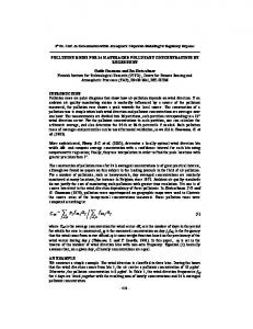
Fig 1 Making a correspondence between space and time
output
training signal
ideal output actual output
output x
layered neural network sensory signals
t
d 2x →0 dt 2
Fig. 2 Temporal Smoothing Learning
AAAA AAAA AAAA AAAA
robot
motion generator state evaluator
actuator
motion state m x environment sensor
Temporal Smoothing Learning is a simple learning algorithm to make a correspondence from space to time as shown in Fig. 1. Here the spatial information is defined as the information that is represented by the present sensory signals. We also use ‘state’ in the same meaning here. The spatial information itself has no information about time. However, if we assume that the real world changes its state determinisiticly, there exists an temporal order in which each state appears according to the relation of cause and effect. We think that it is important to extract the temporal relation among the states. Temporal Smoothing Learning is useful for realizing it. Temporal Smoothing Learning is so simple that the output curve of a layered neural network, whose inputs are sensory signals, is trained to become smooth along time as shown in Fig. 2. To put it concretely, the absolute value of the second time derivative of the output is trained to decrease, and the output curve becomes close to a straight line. Then the output has one-to-one correspondence to the time. This means that the output represents the temporal information. This learning algorithm can be used not only for estimating the necessary time to get a reward in reinforcement learning, but also for integrating the signals from many sensory cells, each of which has only a local receptive field like retina[6][7]. For example, when an object is in a simple oscillation on the visual field and the signals from the local visual cells arranged in a row are put into the neural network as the inputs, the output becomes to represent the object location through this learning without any supervised signals.
(T+7)
2
reinforcement evaluation value Φ signal Fig. 3 Structure of the reinforcement learning system prediction, Constant Evaluation Slope Learning, which is an extension of Temporal Smoothing Learning, is employed here. In this learning, the ideal change of the evaluation value in one time unit, is calculated from the maximum necessary time Nmax as ∆Φ ideal = Φ amp / Nmax
(1)
where Φ amp is an ideal amplitude of the evaluation value. Here since the value range of every neuron’s output is from -0.5 to 0.5, Φ amp is set to be 0.4-(-0.4)=0.8. For adaptability, Nmax is calculated as Nmax[i] = max{(1-1/τ)Nmax[i-1], N[i]}
(2)
where N[i] is the necessary time at the i-th trial, and τ is a large time constant. Then by comparing the change of the actual evaluation value with the ideal one, the evaluation value at the previous time Φ(t-1) is trained by the training signal as Φs(t-1) = Φ(t-1) - η (∆Φideal - ∆Φ(t))
(3)
where Φ s is the training signal for the evaluation value, ∆Φ(t) = Φ(t) - Φ(t-1), and η is a training
constant. By this learning, the evaluation curve along time becomes smooth and the slope of the curve becomes constant not depending on the trial. When the robot arrives at the target state, the evaluation value is trained to become 0.4. The robot generates its motions according to the sum of the outputs of the motion generator m , and random numbers rnd as trial and error factors. The motion signals m are trained by the training signals as m s = m + ζ rnd ∆ Φ
(4)
where ζ is a training constant. By this learning, the motions are trained for the robot to get more gain of the evaluation value. This learning is processed in parallel with the evaluation learning. The neural network is trained by Back Propagation learning[8] according to the training signals as Eq. (3) and (4) at every time step. This type of reinforcement learning is very similar to TD type reinforcement learning. The main difference is the shape of the ideal evaluation curve along time. In TD type reinforcement learning, it is exponential curve, while it is a straight line in our learning. It can be said that the necessary time to the target state is predicted as the evaluation value also in TD type reinforcement learning. From the other viewpoint, our learning can be thought as a special case of TD type reinforcement learning[2] in the regard that the discount factor γ for calculating a weighted sum of the reinforcement signals in the future is 1.0 and the system has a small constant penalty -∆Φideal at every time step. One of the reasons to employ Temporal Smoothing based reinforcement learning is that Temporal Smoothing Learning has been confirmed to have an ability to integrate local visual sensory signals into an analog spatial information without any supervised signals[6][7] as in the previous section. Another reason is that the adaptive modification method of the ideal slope of the evaluation curve along time ∆Φ ideal has been proposed in the learning as shown in Eq. (1) and (2). The ideal slope ∆Φ ideal corresponds to the discount factor γ in TD type reinforcement learning at the first viewpoint of the comparison in the previous paragraph.
3. Acquisition of Appropriate Motions not Depending on the Target Size
local receptive field without overlapping with the other cells, and generates an output as the area ratio occupied by the projected target in its receptive field. It is assumed that this robot obtains a reward only when the robot reaches the target object. To put it concretely, it obtains a reward when the robot goes through the center of the target object. The length of the robot, from the left wheel to the right wheel, is 2.0, and the diameter of the target is varied from 1.0 to 2.0. Figure 5 shows the signal flow of this simulation. We used a three layered neural network, that composed of 96 input neurons, 40 hidden neurons and 3 output neurons. All of hidden and output neurons had sigmoidal output function whose value range is from -0.5 to 0.5. Since all the connection weights from the hidden layer to the output layer were set to be 0.0 before the learning, the output values of the neural network were 0.0 not depending on the inputs. In this case, the number of outputs for the motion signals were two, and the robot rotated its wheels according to the outputs. The range of the evaluation value is also from -0.5 to 0.5. The evaluation value before the learning was 0.0 for every relative target location from the robot. When the robot reached the target or missed it, one trial finished. Here the miss means that the
Y 7.0
Y'
size 1.0 < d < 2.0
loco m robootive t
X'
48 cells
Fig. 4
5.0 X
start point visual sensor
-5.0
48 cells
Simulation environment in the “going to target” task with various target size. main signal flow d dt rnd1 2
d dt 2
~
signal flow for learning rnd2 ~
+ +
3.1 Task As shown in Fig. 4, we gave a task to a locomotive robot with two wheels and two visual sensors to go to an target object while the size of the target object is varied. One of the two visual sensors is located on the left wheel and the other is located on the right wheel. Each visual sensor has 48 visual cells, those are arranged in a row, and has a total of 180 degree of visual field. Each visual cell has only a
target object
evaluation value
motion signals
visual sensory signals Fig. 5 Signal flow of the simulation
target image disappears from the visual field of the robot without reaching the target. Then the target size was changed randomly and the target was located at another place chosen randomly. If the robot missed the target, the evaluation output was trained to be -0.4. In the early phase of the learning, the target was located only within the range that was close to the robot, since the robot was moved by the random numbers. According to the progress of the learning, the range of the initial target location becomes wider gradually until -5 ≤ X ≤5, 0 ≤ Y ≤ 7. Here the ideal evaluation function does not depend on the target size, but depends only on the relative target location from the robot. Therefore, to obtain the ideal evaluation function, spatial recognition using stereo vision is required.
route for the largest target route for the smallest target
Y 8
largest target 4
0 -5
Fig. 6
3.3 Examination of Generalization Ability of the Information in Hidden Neurons The coding of spatial information in hidden neurons and its succession to another learning is examined. The neural network as shown in Fig. 8 is trained by the reinforcement learning using the first three output neurons. After the learning, the last output neuron, which is shown as a circle with dots in
0
start
X
5
The robot’s routes after learning for the largest and the smallest target size. Each point is plotted at every 20 time units.
3.2 Result Figure 6 shows the route of the robot after 300000 trials when the target is located at each of five locations. The lines with squares show the routes when the largest target (diameter is 2.0) is presented and the lines with circles show the routes when the smallest target (diameter is 1.0) is presented. It can be seen that the two routes are very similar to each other. The both routes are almost close to the optimal one such that the robot rotates and then goes straight to the target. However the necessary time to reach the target for the largest target is slightly shorter than that for the smallest one. It can be thought that the visual inputs for the smallest target takes the middle state between that for the large target and that for no targets. Therefore by the generalization ability, the robot cannot go as fast in the case of the smallest target as in the case of the largest one. Figure 7 (a) shows the evaluation values as a function of the target locations and the routes of the robot on the robot centered coordinates when the largest target is presented. In the robot centered coordinates, the target moves relatively on behalf of the robot. Figure 7 (b) shows the case of the smallest target. It can be seen that the evaluation values are almost the same between Fig. 7 (a) and (b). But the value at the same target location is slightly larger in the case of the largest target. The reason can be thought the same as that for the difference in the necessary time as described above. However the difference is far smaller than when only the largest target is presented in the learning. It can be said that the stereo vision is utilized to recognize the distance to the target that does not depend on the target size.
smallest target
Y' 9
target 7 0.5
0.0
-0.5
0 -5
0 robot (a) The largest target
X'
5
Y' 9
target 7
0 -5
0 robot
X' 5
(b) The smallest target Fig. 7
Distribution of evaluation value and robot’s routes after learning in the cases of the largest target and the smallest target in the robot centered coordinates. Each point is plotted at every 10 time units.
Fig. 8, is trained by supervised learning. The last output neuron is connected to the all hidden neurons with 0 connection weight before the learning. Here the generalization of the information about the target location among different sizes of the targets is examined. After supervised learning was applied to the largest target, the output is observed when the
smallest target is presented. The distribution of the training signal is given as shown in Fig. 9. It becomes larger when the target is closer to the robot. For comparison, two other neural networks were prepared. One of them was trained by the reinforcement learning only for the largest target. To the other one, the reinforcement learning was not applied. All these neural networks had the same initial weight values before these learnings. Figure 10 shows the learning curve in the supervised learning in the log scale. y-axis shows the average of the error between the output distribution and the training signal distribution over the area as shown in Fig. 9. It can be seen that the error is reduced faster in the neural networks to which the reinforcement learning was applied beforehand. Furthermore the neural network trained by the reinforcement learning for the largest target only, reduces the error slightly faster
7
0.5
Y'
0.0
0 0 robot
-5
5
-0.5
X Fig. 9 Distribution of the training signal' as a function of the target location for another supervised learning that is applied to the largest target.
7
output for reinforcement learning
output for supervised learning
Y'
AA
0
visual inputs
Error (log)
Fig. 8 Neural network to examine the learning of hidden neurons
0 robot
5 X'
(a) Various size of objects are presented in the reinforcement learning 7
Y'
10 -1
initial error
10 -2
after learning (various size target) no reinforcem ent learning after l earnin g (large target only)
10 -3 10 -4
100000
50000
0
Iteration
Fig. 10 Learning curve in the supervised learning for the largest object. generalization Error
-5
0
-5
0 robot
5 X'
(b) The largest size of object was presented in the reinforcement learning 7
Y'
0.08
after learning rget only) (for the largest ta
0.04
initial error
no reinforcement
learning
after learning (for various sizes of targets)
0
0.00 0
50000
100000
Iteration
Fig. 11 The change of error between the output when the smallest target is presented and the supervised signal given for the largest target.
-5
0 robot
5 X'
(c) Reinforcement learning was not applied Fig 12
Output distribution as a function of the smallest target location after the supervised learning for the largest target.
than that trained for the various sizes of the targets. Figure 11 shows the change of the average difference between the training signals for the largest target and the outputs when the smallest target are presented. It is plotted in the linear scale. The difference is called generalization error here. It is interesting that the generalization error decreases once and then increases over the initial error when the neural network is trained by the reinforcement learning for the largest target and when the reinforcement learning was not applied beforehand. The difference increases more in the former case than in the latter case. The initial error means the average of the difference between the training signals and 0. It can be thought that the similar state to the “over training” has happened. Figure 12 shows the output distribution as a function of the smallest target locations. In the network trained with a various sizes of targets, the output distribution is not so smooth but the value is closer to the training signal than in the other cases. The generalization ability of the information about the distance from the robot to the target among the different sizes of the targets was observed. It can be thought that the information for the perception of the distance to the target, which did not depend on the target size, is stored in the hidden neurons through the reinforcement learning for a various sizes of targets.
obstacle
locomotive robot left
target object
total 48 inputs right
12 cells
12 cells
12 cells
12 cells
for the target for the obstacle
Fig. 13 “Going to a target” task with an obstacle
target
robot
8
6
4
2
4. Obstacle Avoidance
start
0 -5
-4 -3
4.1 Task Here we gave another task to the same locomotive robot used in the previous chapter. The robot has to reach the target while avoiding an obstacle as shown in Fig. 13. It has total of 4 visual sensors. Two of them catch only the target object and the others catch only the obstacle. It is assumed that they can catch the target or obstacle even if it hides behind the other one. One sensor for the target and one sensor for the obstacle are attached on the left wheel and the other pair of the sensors are attached on the right wheel. Each visual sensor had 12 visual sensory cells which cover 180 degree of visual field without overlapping. The total of 48 visual signals are given to the input layer of the neural network. The neural network has two hidden layers. The lower one has 30 neurons and the upper one has 20 neurons. The robot cannot go through the obstacle. This means that the robot stops its motions when it collides with the obstacle even if the motion signals are not 0. But it has no penalty for the collisions. The diameters of the target and the obstacle are both 1.0 and the length of the robot is 2.0. Initial obstacle location is chosen randomly in the range of -5 ≤ x ≤5, 0 ≤ y ≤ 7 that is the same as the target location range, but it is not located at the area where the distance from the target is smaller than 2.0. Furthermore, the obstacle is not located until the learning progresses and the initial target location is
-2 -1
0
1
2
3
4
5
(a) with no obstacles
AA AAA AAA AAA AAA
When the target object is located
at at
, the robot stops to move , the robot collides with the obstacle
The target was not initially located close to the obstacle (in the large circle) at the learning phase.
8
6
obstacle
4
2
0
-5 -4
-3 -2
-1
0
1
2
3
4
5
(b) with an obstacle Fig. 14
Comparison of the robot’s routes after learning between in the task with an obstacle and with no obstacles.
spread to the final range. After the robot finishes one trial, the target and the obstacle are located respectively at another place chosen randomly.
4.2 Result Figure 14 shows the robot’s routes after 167000 trials (the best data until 200000) in two cases. In the first case (Fig. 14 (a)), there are no obstacles in the visual field of the robot. In the second case (Fig. 14 (b)), an obstacle is located in front of the robot’s start position. The large circle in Fig. 14 (b) shows the area where the target was not located in the learning phase because the distance from the target to the obstacle is smaller than 2.0. The area filled with dots shows the initial target locations where the robot could not reach the target. It stopped its motions near the start position of the robot. The hatched area shows the initial target locations where the robot collided with the obstacle and trapped after some motions from the start. Except for the small areas mentioned above, the robot could avoid the obstacle effectively and reach the target. And the route is obviously different between when the obstacle exists and when it does not exist. In the case of no obstacle, the robot’s routes are different from the optimal ones, in which the robot rotates until it catches the target in the center of the visual sensor and go straight toward the target like the routes in Fig. 6 in the simulation in the previous chapter. The reason can be thought that the size of the neural network is not large enough. Another thing that have to be mentioned about this learning is that the learning is not so stable that the area of the initial target location where the robot could not reach, moved and changed its shape dynamically according to the progress of the learning. Figure 15 shows the distribution of evaluation value as a function of the target locations in the robot centered coordinates when the obstacle was located at (0.0, 3.0). It can be seen that the evaluation value when the target exists behind the obstacle is slightly smaller (see Fig. 7 for reference). Figure 16 shows the evaluation value as a function of the obstacle locations in the robot centered coordinates when the target was located at (0.0, 5.0). It can be seen that the evaluation value is small when the obstacle exists in front of the target. Another thing to be noticed is that the evaluation surface is flat except for the obstacle location area in front of the target. This means that the robot can learn that it is necessary not to go far away from the obstacle but only to avoid the obstacle.
4.3 Examination of Generalization Ability of the Information in hidden neurons Same as the section 3.3, the coding of spatial information in hidden neurons and its succession to another learning are examined. The neural network in Fig. 8 is trained by the reinforcement learning for the first three output neurons. Only the difference is that
Y' 8
0.4 0.3
6
0.2
obstacle
4
0.1
2
0.0 -0.1
0 -5
0
robot
5
X' Fig. 15 Distribution of evaluation value as a function of the target location in the robot centered coordinates when the obstacle is fixed at (0.0, 3.0). Y' 8
0.4 0.3
target
6
0.2
4
0.1 0.0
2
-0.1
0 -5
0
robot
5
X' Fig. 16 Distribution of evaluation value as a function of the obstacle location in the robot centered coordinates when the target is fixed at (0.0, 5.0) it has four layers. Here we examine the generalization ability about the recognition of the state when the target hides behind the obstacle under different locations of the target and the obstacle. As shown in Fig. 17, seven locations for the target (i=0,..,6) and for the obstacle (j=0,..,6) are prepared respectively. The distance from the robot to each of the seven target locations is 5, and that to each of the seven obstacle locations is 3. Then the training signal was given 0.3 in the case of i=j, 0.0 in the case of |i-j|=1, and -0.3 otherwise. i=j means the target exists just behind the obstacle. Then the target location and the obstacle location were chosen randomly except for the case of i=j=a where a is one of (0,..,6), and the neural network was trained by the training signal. a was fixed during the learning. After learning, the visual signals when the both target and obstacle locations were a, were put into the input layer of the network as a test data and the output was observed. Figure 18 (a) shows the output as a function of the target location when the obstacle is fixed at the location 3 when a=3. The solid line with squares shows the output using the hidden neuron trained by the reinforcement learning. The line with circles shows the output using no learning hidden neuron.
The thin line shows the desired output for i=3 and the training signals otherwise. Because the supervised learning is applied except for the location 3, the output is almost the same as the training signal at i=0,1,2,4,5,6. When only one of the target and the obstacle is located at 3, the training signal is not larger than 0.0. Therefore when the both locations are 3, the possibility that the output is smaller than 0.0 is large in general. Actually the output at the location 3 in the case of no learning hidden neurons is far smaller than 0.0. However, the output in the case of the trained hidden neurons is larger than 0.0. Figure 18 (b) shows the outputs as a function of a . The pair (i,j)=(a,a) of the target and obstacle location, was not trained and used as test data. It can be seen that the outputs are larger than 0.0 when the a is 2, 3 or 4 at the case of trained hidden neurons. It is known that the trained hidden neurons had some information about the situation that the target hides behind the obstacle, and the information could be generalized. The reason why the outputs when a is not 2, 3 or 4, are not so large can be thought that the generalization ability is not effective for the biased position.
Y'
target(r=5)
6 4
3
2
4 2
1
5
0
0
6
0 robot 5 obstacle X' (r=3) Fig. 17 The target and obstacle locations in the simulation to examine the generalization ability of the hidden neurons information. -5
after reinforcement learning when no reinforcement learning ideal output 0.5
0.5
0.3
0.3
0.0
0.0
-0.3
-0.3
5. Conclusion Here two tasks to show the effectiveness of the direct-vision-based reinforcement learning were presented. In the first task in which the object size is varied, the robot could obtain an appropriate evaluation function that scarcely depends on the target size after the reinforcement learning. In the second task in which an obstacle is located randomly at every trial, the robot could obtain the motions to avoid the obstacle and go towards the target object. When a supervised learning was applied using the hidden neurons that were trained already through the reinforcement learning, the output for the test data becomes close to the ideal output. That means that the generalization ability became large through the reinforcement learning with respect to the spatial information that was important in the reinforcement learning and was represented on the hidden neurons.
References [1] Kakazu, Y., et al., Annual Report of Research on Theory of Adaptive and Reinforcement Learning, “System Theory of Function Emergence” under the Grant-in Aid for Scientific Research on Priority Area supported by the Ministry of Education, Science, Sports and Culture of Japan, 1997 [2] Barto, A. G., Sutton, R. S. and Anderson C. W., “Neuronlike Adaptive Elements That Can Solve Difficult Learning Control Problems”, IEEE Trans. SMC-13, pp. 835-846, 1983 [3] Watkins, C. J. C. H. and Dayan, P., “Q-learning”, Machine Learning, Vol. 8, pp. 279-292, 1992
-0.5
-0.5 0
3
6
0
3
6
a i (target location) (a) the output as a function of (b)the output as a function the target location when of the location a of the the obstacle is fixed at j=3. test data.
Fig. 18 Comparison of the output after supervised learning between the trained hidden neurons and no trained ones.
[4] Asada, M., Noda, S., Tawaratsumida, S. and Hosoda, K., “Purposive Behavior Acquisition for a Real Robot by Vision-Based Reinforcement Learning”, Machine Learning, Vol. 24, pp. 279-303, 1996 [5] K. Shibata and Y. Okabe, “Reinforcement Learning When Visual Sensory Signals are Directly Given as Inputs”, Proc. of ICNN '97 Houston, Vol. 3, pp. 1716-1720, 1997 [6] K. Shibata and Y. Okabe, “Unsupervised Learning Method to Extract Object Locations from Local Visual Signals”, Proc. of ICNN '94 Orlando, Vol. 3, pp. 1556-1559, 1994 [7] K. Shibata and Y. Okabe, “Integration of Local Sensory Signals and Extraction of Spatial Information Based on Temporal Smoothing Learning”, Journal. of JNNS, Vol. 3, No. 3, pp. 98-105, 1996 (in Japanese) [8] Rumelhart, D. E., Hinton, G. E. and Williams, R. J., “Learning representation by back-propagating errors”, Nature, Vol. 323, No. 9, pp. 533-536, 1986