Hindawi Publishing Corporation International Journal of Distributed Sensor Networks Volume 2015, Article ID 264064, 10 pages http://dx.doi.org/10.1155/2015/264064
Research Article Direction-of-Arrival Estimation of Virtual Array Signals Based on Doppler Effect Feng Zhao, Xia Hao, and Hongbin Chen Key Laboratory of Cognitive Radio and Information Processing, Guilin University of Electronic Technology, Ministry of Education, Guilin 541004, China Correspondence should be addressed to Hongbin Chen;
[email protected] Received 5 December 2014; Accepted 13 January 2015 Academic Editor: Qilian Liang Copyright © 2015 Feng Zhao et al. This is an open access article distributed under the Creative Commons Attribution License, which permits unrestricted use, distribution, and reproduction in any medium, provided the original work is properly cited. The estimation accuracy of direction-of-departure (DOD) and direction-of-arrival (DOA) is reduced because of Doppler shifts caused by the high-speed moving sources. In this paper, an improved DOA estimation method which combines the forwardbackward spatial smoothing (FBSS) technique with the MUSIC algorithm is proposed for virtual MIMO array signals in high mobility scenarios. Theoretical analysis and experiment results demonstrate that the resolution capability can be significantly improved by using the proposed method compared to the MUSIC algorithm for the moving sources with limited array elements, especially the DOA which can still be accurately estimated when the sources are much closely spaced.
1. Introduction In the last several decades, the high resolution directionof-arrival (DOA) estimation methods using antenna arrays have played an important role in various fields, including mobile communications, radar, sonar, and seismology (a few examples of the many possible applications). For example, public safety communications systems can also benefit from DOA methods for search and rescue operations based on estimated DOAs from victim mobile devices [1]. There are less reflector and direct path dominating in high mobility scenarios. Although Doppler diffusion is not outstanding, but the Doppler shift is more serious, which could affect the symbol detection for the wireless digital communication system, and even leads to significant degradation of the communication quality. The system performance can be improved by these methods that include the augment of the transmission power and signal-to-noise ratio or the decrease of communication link distance, but these methods are limited in practical applications. Nevertheless, it is a grand challenge when we take the extension of antenna aperture on the small aircraft into consideration to improve the resolution ratio of the system. Therefore, it is necessary to improve the resolution of multiple sources by combining the virtual
method of the extended array elements with existing MIMO technology in high mobility scenarios. The virtual array was formed to extend the equivalent array aperture by using the conjugate counterpart of the array output, so that it can handle more sources than the original arrays [2]. Antenna arrays can obtain additional freedom by exploiting virtual antenna arrays, which led to narrower beam width and lower side lobes [3, 4]. However, they did not consider the correlation between the signals, so some scholars consider the decorrelation of received signals firstly and then estimate the DOA with estimation algorithm in hand to improve resolution ratio [5–7]. In addition, the DOD was estimated by using an ESPRIT algorithm with two-dimensional direction search method and the DOA was estimated by using a ROOT-MUSIC algorithm with one-dimensional search method are not only complicated to calculate, but need extra angle matching [8]. But it has been shown that the DOD and DOA could be estimated by using one-dimensional search method in [9], which avoid nonlinear search of 2D spectrum peak and iteration calculation; thus the method reduced computational complexity greatly without losing accuracy and at the same time parameters can be paired automatically. And DOA was estimated by using a modified MUSIC algorithm based on virtual array
2 transformation and spatial smoothing technique [10–12], which avoided seeking the peak of the spectrum of traditional MUSIC. Moreover, the new DOA estimation algorithm [13] was proposed, which made full use of weighted spatial smoothing combining the autocorrelation information with cross-correlation information of the submatrix. At the same time, the DOA estimation algorithm of coherent sources was proposed by using the ESPRIT algorithm and the MUSIC algorithm with multiple and invariant features [14, 15]. However, these literature have only done virtual extension for receiver arrays. Few of them considered the problem of combining virtual MIMO arrays with the MUSIC algorithm (using the FBSS technique) in high mobility scenarios. So this work will study the DOD-DOA estimation which can be applied to angle estimation of high-mobility sources by combining the virtual array transformation with the MUSIC algorithm (using FBSS processing), which can choose flexibly the number of virtual array elements and their locations according to the actual environment. Moreover, our proposed approach can improve localization precision effectively in case of the sources with similar angle and limited array elements. This paper has the following five parts. The system model and the mathematical expression for the virtual array signals are provided in Section 2. The proposed MUSIC algorithm by using FBSS processing with a detailed analysis of its decorrelation effect is investigated in Section 3. Simulation results are presented in Section 4 and conclusions are drawn in Section 5.
International Journal of Distributed Sensor Networks
dt S0
S1 Ψ The virtual uniform linear array S−1
𝜃
dr
··· y2
y1
y3
··· y4
yn
The receiver arrays
Figure 1: Virtual uniform linear array model.
the transmitted signals are represented as 𝑠−1 (𝑡) = 𝑠1∗ (𝑡). The complex conjugate output of the 𝑚th element can be written as 𝑀
2. Virtual Array Model Array dates or information of virtual location was constructed to achieve the goal of array extension based on the received signals of actual arrays, which is called virtual arrays extension technology [2]. But the number of antenna elements is limited by apertures of platform in high mobility scenarios, so resolution is improved by using the virtual array extension technology. 2.1. Virtual Aperture Extension. Assume that two antennas are installed in the plane with the limited volume, black antenna 𝑠0 (𝑡) and 𝑠1 (𝑡) express real-time position of plane and white antenna. 𝑠−1 (𝑡) is the virtual antenna at one moment, at the same time 𝑠−1 (𝑡) and 𝑠1 (𝑡) are the center symmetry about 𝑠0 (𝑡). The transmitter arrays are composed of two uniform linear array elements (ULA), and receiver comprised 𝑁 ones as shown in Figure 1. Element spacing of transmitter and receiver are 𝑑𝑡 and 𝑑𝑟 , respectively. Virtual MIMO system model of transmitter and receiver is shown in Figure 1. Suppose that there are 𝐾 sources close to the receiver at a constant 𝑉 rate in the air. The DOD and DOA of the 𝑘th source are represented as 𝜙𝑘 , 𝜃𝑘 , respectively. The mutually orthogonal narrow-band coding signals are emitted for the transmitted signals which are represented as {𝑠0 (𝑡), . . . , 𝑠𝑀(𝑡)}. Suppose that virtual array are symmetrical extrapolation values about the position of real elements; namely,
∗ ∗ ∗ 𝑥𝑚 (𝑡) = ∑ 𝑠𝑚 (𝑡) 𝑒−𝑗(𝑚−1)2𝜋𝑑𝑡 /𝜆 sin(𝜑𝑚 ) + 𝑛𝑚 (𝑡) 𝑚=1 𝑀
(1)
∗ = ∑ 𝑠𝑚 (𝑡) 𝑒−𝑗(𝑚−1)2𝜋𝑑𝑡 /𝜆 sin(𝜑𝑚 ) + 𝑛𝑚 (𝑡) . 𝑚=1
∗ Obviously, 𝑥𝑚 (𝑡) can be considered as the output signals of the virtual elements. Therefore, by concatenating the actual array output signal and its conjugate components, the new array output vector [2] can be written as
y (t) = [
TA∗ Tn∗ (t) Tx∗ (t) ]=( ) ) s (t) + ( x (t) n (t) A
(2)
̃ (t) + v (t) , = As ̃ = [a(𝜙1 ), a(𝜙2 ), where T = IM (𝑀 − 1 : 1, :) and A a(𝜙𝑀)] is the direction matrix of the virtual array, whose 𝑚th column denoted as a(𝜙𝑚 ) = [𝑒−𝑗(𝑚−1)2𝜋𝑑𝑡 /𝜆 sin(𝜙𝑚 ) , . . . , 1, . . . , 𝑒𝑗(𝑚−1)2𝜋𝑑𝑡 /𝜆 sin(𝜙𝑚 ) ]𝑇 ∈ (1 ≤ 𝑚 ≤ 𝑀) is the corresponding extended array steering vector. 2.2. Received Signal with Doppler Frequency Shift. The Doppler frequency is less than zero when the sources are far away from the receiver. In other words, the frequency of the received signal is less than the frequency of the transmitted signal, and vice versa. Consider a single transmitted source
International Journal of Distributed Sensor Networks
3
firstly. Delay of the actual transmitted signals arriving at a certain receiver can be written as 𝜏=
𝑑𝑡 sin 𝜃 V𝑡 sin 𝜃 = . 𝑐 𝑐
(3)
Phase difference of transmitted arrays arriving at receiver can be obtained as 𝜑(𝑡) = 𝜔0 𝜏 = 2𝜋(V𝑡 sin 𝜃/𝜆) which is a function of 𝑡. When the radial velocity is constant, Doppler is caused with the frequency difference 𝜑(𝑡), which can be expressed as 𝑓𝑑 =
V𝑓 1 𝑑𝜑 V = sin 𝜃 = 0 sin 𝜃. 2𝜋 𝑑𝑡 𝜆 𝑐
(4)
It is straightforward to obtain expression of 𝑁 received signals as 𝑦 (𝑡) = [𝑦 1 (𝑡), 𝑦 2 (𝑡), . . . , 𝑦𝑁 (𝑡)] = 𝛼 exp (𝑗2𝜋𝑓𝑑 𝑡) b𝑟 (𝜃) ×
𝑇
aT𝑡
(𝜙) × s (𝑡) + n (𝑡) .
(5)
The array direction vector [8] in the transmitter can be written as a𝑡 (𝜙) = [𝑒𝑗2𝜋(𝑀−1)(𝑑𝑡 /𝜆) sin 𝜙 , . . . , 1, 𝑒−𝑗2𝜋(𝑑𝑡 /𝜆) sin 𝜙 ,
2
N
Mixing, filtering, sampling
S2H
S1H
y1,1
Mixing, filtering, sampling
H SK
y2,1
S1H
yk,1
S2H
y1,N
H SK
y2,N
yK,N
Figure 2: Matched filtering of the receiver array.
and b𝑟 (𝜃𝑘 ) as the steering vectors and the 𝑀 × 𝐾 and 𝑁 × 𝐾 size are represented as transmitted arrays manifold matrix A = [a𝑡 (𝜙1 ), a𝑡 (𝜙2 ), . . . , a𝑡 (𝜙𝑘 )] and received arrays manifold matrix B = [b𝑟 (𝜃1 ), b𝑟 (𝜃2 ), . . . , b𝑟 (𝜃𝑘 )], respectively. 𝑇𝑆 is the duration time of each symbol, and 𝑁 is a 𝑁 × 𝐿 noise matrix. Λ = diag(𝑐) is a 𝐾 × 𝐾 diagonal matrix, where c = [𝛼1 exp(𝑗2𝜋𝑓𝑑1 𝑙𝑇𝑆 ), 𝛼2 exp(𝑗2𝜋𝑓𝑑2 𝑙𝑇𝑆 ), . . . , 𝛼𝑘 exp(𝑗2𝜋𝑓𝑑𝑘 𝑙𝑇𝑆)].
(6)
𝑇
𝐿𝑒−𝑗2𝜋(𝑀−1)(𝑑𝑡 /𝜆) sin 𝜙 ] .
3. Proposed Algorithm
The array direction vector in the receiver can be written as 𝑇
b𝑟 (𝜃) = [1, 𝑒−𝑗2𝜋(𝑑𝑟 /𝜆) sin 𝜃 , 𝐿𝑒−𝑗2𝜋(𝑁−1)(𝑑𝑟 /𝜆) sin 𝜃 ] ,
(7)
where n(𝑡) = [n1 (𝑡), n2 (𝑡), . . . , n𝑁(𝑡)]𝑇 ∈ (𝑁 × 𝐿) is the noise matrix, whose each component (𝑁 × 1) is assumed to be independent, zero mean, complex, and Gaussian distributed. 𝛼 is the amplitude attenuation factor with the transmission path, a𝑡 (𝜙𝑖 ) is the path response of array from the 𝜙𝑖 direction, and b𝑟 (𝜃𝑖 ) is the path response of array from the 𝜃𝑖 direction. In the case of multiple targets, the angles of the transmitting arrays and receiving arrays are (𝜙1 , 𝜙2 , . . . , 𝜙𝐾 ) and (𝜃1 , 𝜃2 , . . . , 𝜃𝐾 ), respectively, 𝑓𝑑𝑘 is the Doppler shift of the 𝑘th target, and received signals at the time 𝑡 can be expressed as 𝐾
y (𝑡) = ∑ 𝛼𝑘 exp (𝑗2𝜋𝑓𝑑𝑘 𝑡) b𝑟 (𝜃𝑘 ) ⋅ a𝑇𝑡 (𝜑𝑘 ) ⋅ s (𝑡) + n (𝑡) . 𝑘=1
(8) And then (8) is discretized and expression of received arrays [16] can be denoted as 𝐾
y = ∑ 𝛼𝑘 exp (𝑗2𝜋𝑓𝑑𝑘 𝑙𝑇𝑠 ) b𝑟 (𝜃𝑘 ) ⋅ a𝑇𝑡 (𝜑𝑘 ) s + n (𝑙𝑇𝑠 ) 𝑘=1
1
(9)
𝑇
= BΛA S + N, where the size of receive signal y is 𝑁 × 𝐿 and 𝑙 ∈ (1, 𝐿) is the number of snapshots within a single pulse. Transmitted signal 𝑆 = [𝑠1 , 𝑠2 , . . . , 𝑠𝑚 ]𝑇 is a 𝑀 × 𝐿 matrix. Defining a𝑡 (𝜙𝑘 )
Received signals are superposition of 𝐾 sources, which arrive in 𝑁 received antennas. Assume that there are 𝐾 × 𝑁 matched filter in the receiver. Then, each signal is separately isolated from the received signal by adopting modern digital signal processing technology such as mixing, filtering, and sampling. Because the signal satisfies orthogonality, there are 1, 1 𝐿 ∑𝑆 (𝑙) 𝑆𝑗∗ (𝑙) = { 0, 𝐿 𝑙=1 𝑖
𝑖=𝑗 𝑖 ≠ 𝑗.
(10)
Then the 𝐾 × 𝑁 independent output signal yk,n is obtained by multiplying the separated received signals y by the transmit𝐻 . The matched filtering structure [16] ted signal 𝑆1𝐻, 𝑆2𝐻, . . . , 𝑆𝐾 is shown in Figure 2. The output of 𝑙 sample point after the relevant processing of receiver at a time is written as Y = yS𝐻 = BΛA𝑇SS𝐻 + WS𝐻 = BΛA𝑇 + N
(11)
according to the column vector; the 𝑁 × 𝑀 matrix Y can be ̂ turned into 𝑀𝑁 × 𝐿 dimensional vector Y ̂ = (A ⊕ B) c𝑘 + N, ̂ Y
(12)
̂ = vec(Y), N ̂ = vec(N), the ⊗ is Kronecker where Y product, vec(⋅) is matrix which was written as a column vector ̂ = vec(N) from left to right, according to the principle N and A ⊕ B = [a𝑡 (𝜑1 ) ⊗ b𝑟 (𝜃1 ), a𝑡 (𝜑2 ) ⊗ b𝑟 (𝜃2 ), . . . , a𝑡 (𝜑𝑘 ) ⊗ b𝑟 (𝜃𝑘 )]. So the total output signal matrix after matched filter is represented as 𝐾
̃ = ∑ (A ⊕ B) C + N, ̃ Y 𝑘=1
(13)
4
International Journal of Distributed Sensor Networks
̂ is a 𝑀𝑁 × 𝐿 where the 𝐶 = [∑𝑘𝑘=1 𝑐𝑘 ] is a 1 × 𝐿 matrix, the N matrix, the A ⊕ B is 𝑀𝑁 × 1 matrix, and C contains the target scattering coefficient and Doppler shifts information. First received signals are divided into two subspaces [11, 17]; namely, they are divided into array element 𝑥0 with ̃ : 𝑁𝑟 , :) and array element 𝑥1 ̃ 1 = Y(1 carried information Y ̃ 2 = Y(𝑁 ̃ 𝑟 : 2𝑁𝑟 , :). Then, the with carried information Y ̃1 is expressed as covariance matrix of first submatrix 𝑌 ̃ 1Y ̃ 𝐻] . R11 = 𝐸 [Y 1
(14)
Mutual covariance of two submatrix can be given as R21 =
̃ 2Y ̃1 Y . 𝐿
(15)
The singular value decomposition (SVD) [18] is performed for the autocorrelation matrix R11 , namely, [U, S, V] = SVD(R11 ). The reconstructed covariance matrix by the SVD of the R11 is denoted as R11 = VS−1 U𝐻.
vector of the coherent signals transforms into the noise subspace, resulting in performance being deteriorated. So some direction vectors of coherent signals and noise subspaces are not orthogonal, for which we cannot estimate the DOA of coherent signal by using high resolution feature decomposition algorithm [7, 13]. In the preprocessing of the coherent signals, it is necessary to remove the correlation by using a spatial smoothing [12–14] with reducing dimension method between signals. The modified algorithm can be described as follows. We consider that the received signals can remove the correlation. Forward-backward spatial smoothing (FBSS) is used to preprocess the data of the received arrays. After the ̂ performs subspace classification [17], then received signal Y ̂ : 𝑁𝑟 , :) carried ̂ 1 = Y(1 we divide it into the information Y ̂ 2 = Y(𝑁 ̂ 𝑟 : 2𝑁𝑟 , :) carried by by 𝑥0 and the information Y 𝑥1 , respectively. So covariance matrix of forward subarray of array elements 𝑥0 in which the number of snapshots is 𝑙 can be obtained as ̂ lY ̂ 𝐻] . R𝑥 = 𝐸 [Y l
(16)
Mixed covariance by extracting the signal subspace are represented as R = R21 R11 .
Define the covariance matrix of the forward spatial smoothing as
(17) R𝑥 =
Mixed covariance R of expression (17) by using eigenvalue decomposition is expressed as [𝜗, D] = eig (R) ,
(18)
𝑘 = 1, 2, . . . , 𝐾.
(19)
Signal subspace 𝜗𝑠 = 𝜗(:, 1) is extracted from feature vectors 𝜗 which is decomposed by R and subspace is processed as follows: ̂ = 𝜗𝑠 (2 : 𝑁𝑟 , :) . 𝜗 𝑠 𝜗𝑠 (1 : 𝑁𝑟 − 1, :)
(20)
Therefore, the DOA can be expressed as 𝑐 ̂ )) angle (𝜗 𝜃𝑘 = arcsin ( 𝑠 2𝜋𝑑𝑓0
𝑘 = 1, 2, . . . , 𝐾.
(21)
The DOA is estimated by further precise processing with the formula (21) 𝑁 −1
1 𝐿 ∑R . 𝐿 𝑙=1 𝑥
(24)
In the same way, we can obtain the covariance matrix of backward spatial smoothing as
where D = diag[𝑒−𝑗2𝜋𝑑𝑡 𝑓0 sin 𝜙/𝑐 , 0, . . . , 0]𝑁𝑟 ×𝑁𝑟 . Thus, the DOD [7–9] can be given as 𝑐 angle (D)) 𝜑̂𝑘 = arcsin ( 2𝜋𝑑𝑓0
(23)
R𝑏 = JR𝑥 ∗ J, 0 0 ⋅⋅⋅ 0 ⋅⋅⋅ 1 . . . .. .. 1 0 ⋅⋅⋅
where J = [ ..
1 0 . .. ] . 0 𝑁𝑟 ×𝑁𝑟
(25)
The conjugate of R𝑥 is R𝑥∗ .
Therefore, we can define forward-backward smoothing covariance matrix [5] as R𝑥𝑥 =
1 (R + R𝑏 ) . 2 𝑥
(26)
Overestimate operation on the processed covariance can be obtained as R11 =
−1 𝐻 1 2 𝐻 R𝑥𝑥𝑚 ) R𝑥𝑥𝑚 , ∑ R𝑥𝑥𝑚 (R𝑥𝑥𝑚 2 𝑚=1
(27)
where R𝑥𝑥𝑚 = R𝑥𝑥 (:, 𝑚 : 𝑁𝑟 + 𝑚 − 2). The steps for the proposed algorithm are given as follows.
(22)
̂ into two subarrays: Y ̂1 = Step 1. Divide the received signal Y ̂ 2 = Y(𝑁 ̂ 𝑟 : 2𝑁𝑟 , :). ̂ : 𝑁𝑟 , :) and Y Y(1
The receiving signals of arrays are coherent through the above algorithm analysis, for which the dimensions of the signal subspace can only reflect direction of arrival of the irrelevant signals. In other words, corresponding characteristic
̂ 1 can Step 2. Autocorrelation matrix R11 of the subarray Y be obtained by using the formula (27), and cross-correlation matrix R21 of the two subarrays can be get by using the formula (15).
𝜃̂𝑘 =
𝑟 1 ∑ 𝜃𝑘 . 𝑁𝑟 − 1 𝑘=1
International Journal of Distributed Sensor Networks DOD-DOA two transmission arrays
20
20
15
15
10
10
5
5
0 −5
0 −5
−10
−10
−15
−15
−20
−20
−25 −70 −60 −50 −40 −30 −20 −10 DOD (deg)
0
DOD-DOA three transmission arrays
25
DOA (deg)
DOA (deg)
25
5
10
20
30
First source Second source Third source
−25 −30
−20
−10
0
10 20 DOD (deg)
30
40
50
First source Second source Third source (a)
(b)
Figure 3: The DOD-DOA estimation performance of three sources.
Step 3. The mixed covariance of signal subspace R can be obtained by using the formula (17). Step 4. The DOA is estimated by using the formula (19) and (22).
4. Simulation Results The actual number of transmitting array and receiving array are set as 𝑀 = 2 and 𝑁 = 2, respectively, and virtual array elements are 𝑀 = 3, element spacing is 𝑑𝑡 = 𝑑𝑟 = 𝜆/2, and 𝐿 = 1024 is code length of transmitted signal. Mutually orthogonal code signals are transmitted for each transmit array element, and the duration time of each code is 𝑇𝑠 = 10 𝜇𝑠. The duration time of the transmitted pulse is 1.024 ms. The amplitude attenuation of 𝐾 target is equal to 1 [16]. Part 1. We consider there are three unrelated targets 𝐾 = 3 existing in the air and the DOA and DOD of three sources are assumed to be located at 𝜙 = (−25∘ , 5∘ , 22∘ ) and 𝜃 = (−22∘ , 18∘ , 5∘ ), respectively. The Doppler shifts are 100 Hz, 1550 Hz, 3000 Hz, respectively, and snapshot 𝐿 is 1024. All simulations are averaged over 1000 independent runs. Figure 3 shows DOD-DOA estimation performance of three signals using our proposed method. It can be seen that the proposed algorithm can accurately estimate the angle of the far spaced sources when SNR = 20 dB. Part 2. The DOA and DOD of three sources are assumed to be located at 𝜑 = (25∘ , 20∘ , 22∘ ) and 𝜃 = (22∘ , 21∘ , 20∘ ), respectively, and the other parameters are the same as before. Figure 4 illustrates that the MIMO Array MUSIC algorithm [10] cannot distinguish the location information when
sources are closed to each other, whatever there are two or three transmitting array elements. Nevertheless, it is evident from Figure 5 that we propose the modified algorithm have also been identified exactly when the three sources are very close. Part 3. Define the root mean squared error (RMSE) of the DOA as RMSE =
2 1 1000 ̂𝑛 1 𝐿 ∑√ ∑ (𝜃 − 𝜃𝑘 ) , 𝐿 𝑙=1 1000 𝑛=1 𝑘
(28)
where 𝜃̂𝑘𝑛 is the estimate of DOA 𝜃𝑘 of the 𝑛th Monte Carlo simulation experiment, 𝐾 is the number of sources. Figure 6 shows the RMSE of DOA estimation as a function of input SNR, and the condition of simulation is the same as first source of Part 1. We can see that DOA estimation performance of different array spacing is very enormous when there are two real arrays or three virtual arrays. As the signal-to-noise ratio increases, the performance of the RMSE of DOA estimation can achieve the optimal when the array interval is 𝑑𝑟 = 𝜆/2. So the performance of the system is best when distance between the adjacent antenna elements are placed with half-wavelength. Part 4. We can see from the Figure 7 that estimation accuracy decreases as the Doppler shift increases. The bigger the Doppler frequency shift, the worse the estimation performance. However, virtual three arrays are better than two arrays for the DOA estimation accuracy. Figure 8 shows the more virtual array elements, the higher estimation accuracy
6
International Journal of Distributed Sensor Networks DOD-DOA two transmission arrays 80
60
60
40 20 DOA (deg)
DOA (deg)
40
DOD-DOA three transmission arrays
20 0
0 −20
−20
−40
−40 −60 −100 −80 −60 −40 −20 0 20 DOD (deg)
40
60
80
−60 −100 −80 −60 −40 −20
0 20 DOD (deg)
100
First source Second source Third source
40
60
80
100
First source Second source Third source (a)
(b)
Figure 4: DOD-DOA estimation performance of three sources (SNR = 25 dB).
DOD-DOA two transmission arrays
25
24
24
23
23
22
22
DOA (deg)
DOA (deg)
25
21 20
21 20
19
19
18
18
17 10
15
20 25 DOD (deg)
30
35
First source Second source Third source
DOD-DOA three transmission arrays
17 −70 −60 −50 −40 −30 −20 −10 DOD (deg)
0
10
20
30
First source Second source Third source (a)
(b)
Figure 5: The DOD-DOA estimation performance of three sources. By using the modified algorithm (SNR = 25 dB).
when the Doppler shift is 𝑓𝑑 = 100 constantly. In addition, Figure 8(a) shows the RMSE of DOA estimation of the three virtual elements superior to the two actual elements with the value of SNR increasing for 𝐿 = 1024 and 𝑓𝑑 = 100. And Figure 8(b) shows the RMSE of DOA estimation of the three virtual elements superior to the two actual elements with the number of snapshots increasing for SNR = 20 and 𝑓𝑑 = 100.
Part 5. By comparing proposed algorithm with the MIMO Array MUSIC algorithm [10], Figure 9 shows performance of the RMSE of DOA estimation as a function of input SNR for the simulation conditions are similar to Part 1, which in case of two real arrays or three virtual arrays, separately. It can be clearly seen from Figure 9 that as the SNR increases, the performance of the proposed method is much better than
International Journal of Distributed Sensor Networks
7 fd = 100 3 transmitter
101
101
100
100
RMSE (deg)
RMSE (deg)
fd = 100 2 transmitter
10−1
10−2 −5
10−1
10−2 0
5
10
15
20
25
30
35
40
−5
0
5
10
SNR (dB) dr = 𝜆/8 dr = 𝜆/4 dr = 𝜆/2
dr = 𝜆/8 dr = 𝜆/4 dr = 𝜆/2
dr = 𝜆 dr = 3𝜆/2
15 20 SNR (dB)
25
30
35
40
30
35
40
dr = 𝜆 dr = 3𝜆/2
(a) DOA
(b) DOA
Figure 6: The RMSE-DOA estimation performance when different interval.
Two transmitter arrays
Three transmitter arrays
101
100 RMSE (deg)
RMSE (deg)
10
0
10−1
10−2
10−2
10−3
10−3 −5
10−1
0
5
fd = 100 fd = 1550
10
15 20 SNR (dB)
25
30
35
40
fd = 3000 CRB
−5
0
5
fd = 100 fd = 1550
(a) DOA
10
15 20 SNR (dB)
25
fd = 3000 CRB (b) DOA
Figure 7: The RMSE-DOA estimation performance of the three sources. In case of different Doppler shift.
the MIMO Array MUSIC one, in addition, which demonstrate that the proposed algorithm can also achieve good performance under the condition of two and three transmitting array elements. Obviously, Figure 10 also shows our proposed algorithm has higher accuracy than the MIMO Array MUSIC algorithm for estimation precision of three sources with the number of snapshots increasing, in case of the two real arrays or three virtual arrays, respectively. At the same time as the number of snapshots increases, estimation accuracy tends to a constant.
5. Conclusion The problem of DOA estimation has been an active research topic in array processing for several decades. In this paper, a new method for virtual array generation and an improved MUSIC algorithm are proposed, which can correctly estimate the two-dimensional angle of sources with limited array elements when the FBSS technique is performed on received signals. Simulation results show that when the virtual array element spacing is equal to the half wavelength, the proposed
8
International Journal of Distributed Sensor Networks First source
First source
10−1 RMSE (deg)
RMSE (deg)
100
10−1
10−2
10−3 −5
0
5
10
15 20 SNR (dB)
25
30
35
40
100
Two transmitter arrays Three transmitter arrays Root CRB
200
300
400
500 600 Snap
700
800
900 1000
25
30
35
40
35
40
35
40
Two transmitter arrays Three transmitter arrays (b) DOA
(a) DOA
The first source 100 −5
0
5
10
15 20 SNR (dB)
25
30
35
40
RMSE (deg)
RMSE (deg)
Figure 8: RMSE-DOA performance under the various numbers of SNR and snapshots.
The first source 100 −5
0
The second source 100 −5
0
5
10
15 20 SNR (dB)
25
30
35
40
The second source
−5
0
10
15 20 SNR (dB)
25
30
35
40
Proposed algorithm MIMO array MUSIC algorithm CRB (a3) DOA two transmitter arrays
RMSE (deg)
RMSE (deg)
The third source
5
5
10
15 20 SNR (dB)
25
30
(b2) DOA three transmitter arrays
100 0
15 20 SNR (dB)
100
(a2) DOA two transmitter arrays
−5
10
(b1) DOA three transmitter arrays RMSE (deg)
RMSE (deg)
(a1) DOA two transmitter arrays
5
The third source 100 −5
0
5
10
15 20 SNR (dB)
25
30
Proposed algorithm MIMO array MUSIC algorithm CRB (b3) DOA three transmitter arrays
(a)
(b)
Figure 9: RMSE of DOA estimation versus SNR.
algorithm can not only estimate the DOA more accurately than the MUSIC algorithm, but also distinguish between closely spaced sources; even the difference of the angle is close to 1 degree.
Conflict of Interests The authors declare that there is no conflict of interests regarding the publication of this paper.
9
The first source 10−1 100
200
300
400
500 600 Snap
700
800
900 1000
RMSE (deg)
RMSE (deg)
International Journal of Distributed Sensor Networks The first source 10−1 100
200
10−1 300
400
500
600
700
800
900 1000
RMSE (deg)
RMSE (deg)
The second source
200
400
500
600
700
800
900 1000
Snap Proposed algorithm MIMO array MUSIC algorithm (a3) DOA two transmitter arrays (a)
RMSE (deg)
RMSE (deg)
300
800
900 1000
The second source 10
100
200
300
400
500
600
700
800
900 1000
(b2) DOA three transmitter arrays
The third source
200
700
Snap
−1
100
500 600 Snap
−1
Snap (a2) DOA two transmitter arrays
10
400
(b1) DOA three transmitter arrays
(a1) DOA two transmitter arrays
100
300
The third source 10
−1
100
200
300
400
500 600 Snap
700
800
900 1000
Proposed algorithm MIMO array MUSIC algorithm (b3) DOA three transmitter arrays (b)
Figure 10: RMSE-DOA versus snapshot curves of three sources (SNR = 20).
Acknowledgments This research was supported by the National Natural Science Foundation of China (61162008, 61172055, 61471135), the Guangxi Natural Science Foundation (2013GXNSFGA019004), the Open Research Fund of Guangxi Key Lab of Wireless Wideband Communication & Signal Processing (12103, 12106), the Director Fund of Key Laboratory of Cognitive Radio and Information Processing (Guilin University of Electronic Technology), Ministry of Education, China (2013ZR02), and the Innovation Project of Guangxi Graduate Education (YCSZ2014144).
References [1] A. Gorcin and H. Arslan, “A two-antenna single RF front-end DOA estimation system for wireless communications signals,” IEEE Transactions on Antennas and Propagation, vol. 62, no. 10, pp. 5321–5333, 2014. [2] M. Lin, L.-L. Cao, J. Ouyang, W. Shi, and K. An, “DOA estimation using virtual array technique for noncirlular signals,” in Proceedings of the International Conference on Wireless Communications and Signal Processing (WCSP ’12), pp. 1–5, October 2012. [3] I. Bekkerman and J. Tabrikian, “Target detection and localization using MIMO radars and sonars,” IEEE Transactions on Signal Processing, vol. 54, no. 10, pp. 3873–3883, 2006. [4] W. Chen, X. Xu, S. Wen, and Z. Cao, “Super-resolution direction finding with far-separated subarrays using virtual array elements,” IET Radar, Sonar and Navigation, vol. 5, no. 8, pp. 824–834, 2011.
[5] K. P. Ray, R. K. Kulkarni, and B. Kasyap Ramkrishnan, “DOA estimation in a multipath environment using covariance differencing and iterative forward and backward spatial smoothing,” in International Conference of Recent Advances in Microwave Theory and Applications (MICROWAVE ’08), pp. 794–796, November 2008. [6] F.-M. Han and X.-D. Zhang, “An ESPRIT-like algorithm for coherent DOA estimation,” IEEE Antennas and Wireless Propagation Letters, vol. 4, no. 1, pp. 443–446, 2005. [7] W. Zhang, W. Liu, J. Wang, and S. Wu, “Joint transmission and reception diversity smoothing for direction finding of coherent targets in MIMO radar,” IEEE Journal on Selected Topics in Signal Processing, vol. 8, no. 1, pp. 115–124, 2014. [8] M. L. Bencheikh and Y. Wang, “Joint DOD-DOA estimation using combined ESPRIT-MUSIC approach in MIMO radar,” Electronics Letters, vol. 46, no. 15, pp. 1081–1083, 2010. [9] J. Li, X. Zhang, and X. Gao, “A joint scheme for angle and array gain-phase error estimation in bistatic mimo radar,” IEEE Geoscience and Remote Sensing Letters, vol. 10, no. 6, pp. 1478– 1482, 2013. [10] A. Zahernia, M. J. Dehghani, and R. Javidan, “MUSIC algorithm for DOA estimation using MIMO arrays,” in Proceedings of the 6th International Conference on Telecommunication Systems, Services, and Applications (TSSA ’11), pp. 149–153, Bali, Indonesia, October 2011. [11] X. Mestre and M. A. Lagunas, “Modified subspace algorithms for DoA estimation with large arrays,” IEEE Transactions on Signal Processing, vol. 56, no. 2, pp. 598–614, 2008. [12] B. Friedlander and A. J. Weiss, “Direction finding using spatial smoothing with interpolated arrays,” IEEE Transactions on Aerospace and Electronic Systems, vol. 28, no. 2, pp. 574–587, 1992.
10 [13] C.-W. Ma and C.-C. Teng, “Detection of coherent signals using weighted subspace smoothing,” IEEE Transactions on Antennas and Propagation, vol. 44, no. 2, pp. 179–187, 1996. [14] M. C. Erturk, J. Haque, W. A. Moreno, and H. Arslan, “Doppler mitigation in OFDM-based aeronautical communications,” IEEE Transactions on Aerospace and Electronic Systems, vol. 50, no. 1, pp. 120–129, 2014. [15] X. Zhang and D. Xu, “Low-complexity ESPRIT-based DOA estimation for colocated MIMO radar using reduced-dimension transformation,” Electronics Letters, vol. 47, no. 4, pp. 283–284, 2011. [16] X. Wang, “Research on signal processing and array design technology in bistatic radar,” Nanjing University of Science and Technology, pp. 7–32, 2014. [17] Z. Xu, “Perturbation analysis for subspace decomposition with applications in subspace-based algorithms,” IEEE Transactions on Signal Processing, vol. 50, no. 11, pp. 2820–2830, 2002. [18] J. Liu, X. Liu, and X. Ma, “First-order perturbation analysis of singular vectors in singular value decomposition,” IEEE Transactions on Signal Processing, vol. 56, no. 7, pp. 3044–3049, 2008.
International Journal of Distributed Sensor Networks
International Journal of
Rotating Machinery
Engineering Journal of
Hindawi Publishing Corporation http://www.hindawi.com
Volume 2014
The Scientific World Journal Hindawi Publishing Corporation http://www.hindawi.com
Volume 2014
International Journal of
Distributed Sensor Networks
Journal of
Sensors Hindawi Publishing Corporation http://www.hindawi.com
Volume 2014
Hindawi Publishing Corporation http://www.hindawi.com
Volume 2014
Hindawi Publishing Corporation http://www.hindawi.com
Volume 2014
Journal of
Control Science and Engineering
Advances in
Civil Engineering Hindawi Publishing Corporation http://www.hindawi.com
Hindawi Publishing Corporation http://www.hindawi.com
Volume 2014
Volume 2014
Submit your manuscripts at http://www.hindawi.com Journal of
Journal of
Electrical and Computer Engineering
Robotics Hindawi Publishing Corporation http://www.hindawi.com
Hindawi Publishing Corporation http://www.hindawi.com
Volume 2014
Volume 2014
VLSI Design Advances in OptoElectronics
International Journal of
Navigation and Observation Hindawi Publishing Corporation http://www.hindawi.com
Volume 2014
Hindawi Publishing Corporation http://www.hindawi.com
Hindawi Publishing Corporation http://www.hindawi.com
Chemical Engineering Hindawi Publishing Corporation http://www.hindawi.com
Volume 2014
Volume 2014
Active and Passive Electronic Components
Antennas and Propagation Hindawi Publishing Corporation http://www.hindawi.com
Aerospace Engineering
Hindawi Publishing Corporation http://www.hindawi.com
Volume 2014
Hindawi Publishing Corporation http://www.hindawi.com
Volume 2014
Volume 2014
International Journal of
International Journal of
International Journal of
Modelling & Simulation in Engineering
Volume 2014
Hindawi Publishing Corporation http://www.hindawi.com
Volume 2014
Shock and Vibration Hindawi Publishing Corporation http://www.hindawi.com
Volume 2014
Advances in
Acoustics and Vibration Hindawi Publishing Corporation http://www.hindawi.com
Volume 2014