On the estimation of target spectrum for filter- array based spectrometers

On the estimation of target spectrum for filterarray based spectrometers Cheng-Chun Chang* and Heung-No Lee Electrical and Computer Engineering, University of Pittsburgh, Pittsburgh PA, USA *Corresponding author: [email protected]

Abstract: Miniature spectrometers have been drawn researchers much attention due to its wide variety of possible applications. In this paper, we show the achievability of a fine spectrometer on-a-chip based on a lowperformance, low-cost filter-array. A low quality filter-array is augmented with digital signal processing techniques. A series of estimators for recovering target spectrum is introduced. By exploiting non-negative nature of spectral content, a non-negative least-square algorithm is found particularly useful for spectrum recovery. The concept is verified in a hardware implementation. ©2008 Optical Society of America OCIS codes: (300.6190) Spectrometers; (120.6200) Spectrometers and spectroscopic instrumentation digital signal processing.

References and links 1. 2. 3. 4.

5. 6. 7. 8. 9. 10.

C. P. Bacon, Y. Mattley, and R. Defrece, “Miniature spectroscopic instrumentation: applications to biology and chemistry,” Rev. Sci. Instrum. 75, 1-16 (2004). D. C. Heinz, and C.-I Chang, “Fully constrained least-squares linear spectral mixture analysis method for material quantification in hyperspectral imagery,” IEEE Trans. Geosci. Remote Sens. 39, 529-546 (2001). O. Manzardo, H. P. Herzig, C. R. Marxer, and N. F. de Rooij, “Miniaturized time-scanning Fourier transform spectrometer based on silicon technology,” Opt. Lett. 24, 1705-1707 (1999). K. Chaganti, I. Salakhutdinov, I. Avrutsky, G. W. Auner, “A simple miniature optical spectrometer with a planar waveguide grating coupler in combination with a plano-convex leng,” Opt. Express 14, 4064-4072 (2006). R. F. Wolffenbuttel, “State-of-the-art in integrated optical microspectrometers,” IEEE Trans. Instrum. Meas. 53, 197-202 (2004). R. Shogenji, Y. Kitamura, K. Yamada, S. Miyatake, and J. Tanida, “Multispectral imaging using compact compound optics,” Opt. Express 12, 1643-1655 (2004). S.-W. Wang, C. Xia, X. Cheng, W. Lu, L. Wang, Y. Wu, and Z. Wang, “Integrated optical filter arrays fabricated by using the combinatorial etching technique,” Opt. Lett. 31, 332-334 (2006). S.-W. Wang, C. Xia, X. Cheng, W. Lu, M. Li, H. Wang, W. Zheng, and T. Zhang, “Concept of a highresolution miniature spectrometer using an integrated filter array,” Opt. Lett. 32, 632-634 (2007). C. L. Lawson and R. J. Hanson, Solving Least Squares Problems, Prentice-Hall, 1974. J. G. Proakis, Digital Communications, McGraw Hill, 2000.

1. Introduction Recently, miniature spectrometers have been drawn researchers great attention. Miniature spectrometers provide solutions to a variety of promising applications in biological, chemical, medical, or pharmaceutical industries, in which small, light-weight, and non-fragile properties of spectrometers are demanded [1, 4-6]. Currently, MEMS, CMOS, micro-optic electromechanical systems, or integrated optics technologies are the main means to build a miniature- or micro- spectrometer. Based on the underlying operation principle, spectrometers can be classified such as grating-based, Fourier-transform based, or filter-based [3-5].

#90677 - $15.00 USD

(C) 2008 OSA

Received 10 Dec 2007; revised 10 Jan 2008; accepted 11 Jan 2008; published 14 Jan 2008

21 January 2008 / Vol. 16, No. 2 / OPTICS EXPRESS 1056

Filter-based static spectrometers utilize different filter functions to filter spectral energy emanating from a target. Recent literatures [6-8] have demonstrated that filter-based spectrometers are capable of high-resolution and allowed to fabricate on-a-chip. By implementing multiple filters and detectors, these spectrometers are avoided to have moving elements, and hence are static and rigid. Furthermore, they have the ability to capture the target spectrum in a very short time. This property is demanded for certain applications especially in biological, biochemical or biomedical industries. For low-cost fabrication, filters may not have delta-function-like shapes with a narrow range response. The spectrum obtained directly from these filtered results is severely distorted, and hence is unacceptable as it is. However, signal processing techniques can be applied to estimate and restore the target spectrum. In this paper, we discuss and provide digital-signal-processing (DSP) methods for filterarray based spectrometers. Based on a discrete linear system model, a series of estimators for spectrum recovery is introduced. By exploiting the non-negative nature of spectral content, we found the non-negative least-squares (NNLS) algorithm particularly useful to estimate and restore the target spectrum with high fidelity. A hardware implementation for the filter-array based spectrometer is demonstrated via a commercialized CCD camera and a DSP board. This prototype shows the achievability of a fine spectrometer on-a-chip based on a lowperformance, low-cost filter-array. Section 2 shows the system model of the filter-array based spectrometer. Section 3 discusses and provides the estimators for restoring a target spectrum. A hardware implementation and experimental results are shown in section 4. Section 5 draws the summary and conclusion. 2. System model of the filter-array based spectrometer light sources s(λ)

Dj(λ) = fj(λ)d(λ)

f1 d

f2 d

fj d

filter-array photoelectric sensor-array

fN d

r j = ∫ D j (λ ) s (λ ) d λ λ

raw data output Signal Processing

Spectrum of the light sources

Fig. 1. System structure of the filter-array based spectrometers

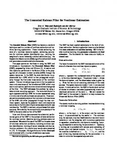
Figure 1 shows the basic system model of the static filter-array based spectrometer. An array of filters is directly placed on top of an array of photoelectric sensors such as CCD sensors. A filter may correspond to a CCD sensor or a group of CCD sensors. The outputs from the CCD sensors are then fed into a digital signal processor. We note that the 1-D structure shown in Fig. 1 can be extended to a 2-D structure straightforwardly by placing filters and CCD sensors in a 2-D plane. In this paper, we will restrict our discussion on the drawn 1-D structure. We assume all the CCD sensors have the same sensitivity function, denoted by d (λ ) , where λ is the continuous wavelength. Denote f j (λ ) as the filter transmission function for jth filter with respect to wavelength λ (each filter may have a different transmission function). A filter and its corresponding CCD sensors compose a spectral detector. The overall sensitivity function of the jth spectral detector can be expressed as D j (λ ) = f j (λ )d (λ ) . For a target with spectral content s (λ ) , the output from the jth detector is rj = ∫ D j (λ )s(λ )d λ . λ

We consider the system and the target spectrum based on a discrete model. The transformation between the target spectrum and the CCD-sensor outputs is associated by the matrix equation #90677 - $15.00 USD

(C) 2008 OSA

Received 10 Dec 2007; revised 10 Jan 2008; accepted 11 Jan 2008; published 14 Jan 2008

21 January 2008 / Vol. 16, No. 2 / OPTICS EXPRESS 1057

r = Hs + n ,

(1)

where

r=

⎡ r1 ⎤ ⎢ ⎥ ⎢ ⎥ ⎢ rj ⎥ ⎢ ⎥ ⎢ ⎥ ⎢r ⎥ ⎣ N⎦

, H=

⎡ D1 (λ1 ) ⎢ ⎢ ⎢ D j (λ1 ) ⎢ ⎢ ⎢ D (λ ) ⎣ N 1

 

 

D1 (λM ) ⎤

 

⎥ ⎥ D j (λM ) ⎥ ⎥ ⎥ DN (λM ) ⎥⎦

, s=

⎡ s (λ1 ) ⎤ ⎢ s (λ2 ) ⎥⎥ ⎢ ⎢ ⎥ ⎢ ⎥ ⎢ ⎥ ⎢ s (λ ) ⎥ ⎣ M ⎦

, and n =

⎡ n1 ⎤ ⎢ n ⎥ ⎢ 2⎥ ⎢ ⎥ ⎢ ⎥ ⎢ ⎥ ⎢n ⎥ ⎣ N⎦

.

The dimensionalities of r, H , s, and n are N ×1, N × M , M × 1, and N ×1 , respectively. r is an observed signal vector whose elements are the outputs of CCD-sensors. The elements in r can be observed simultaneously via each individual detector. n is a noise vector. There are N detectors in this model. H is a detector sensitivity matrix. The M elements in a row of H matrix represent the sensitivity function of a detector, obtained by evenly sampling the sensitivity function over a certain wavelength range. s is a source signal vector, whose elements represent the target spectrum evenly sampled in the wavelength domain. The minimum number of samples required for a given target-spectrum can be obtained through the sampling theorem. That is, consider the shape of the target-spectrum as a continuous function of a unit interval. If B is the minimum value such that the Fourier transform of the function over the unit interval S (θ ) satisfying S (θ ) = 0 for θ > B , 2 B is the minimum number of samples to specify the continuous function [10, p70]. We call these samples resolved points in this paper. The number of resolved points for a given application is critical since it determines the number of required detectors as we will see in section 3. In addition, we note that the sensitivity characteristic of the detectors needs not to be a delta-function shape with a narrow range response. 3. Estimators for restoring the target spectrum Working on the observation vector r , an estimator provides an estimation sˆ of the input spectrum by considering all possible source signal vectors s . One criterion we can use here as the starting point is the maximum a posteriori (MAP) rule [10, p242]. The MAP estimator is obtained by maximizing the posterior probability, i.e., sˆ MAP = arg max P (s | r ) . S

(2)

From the Bayes’ rule, the posterior probability can be written as P(s | r) = P(r | s) P(s) P(r ). When we do not have any information on the source signal such that P (s) is uniformly distributed, the MAP estimator becomes the maximum likelihood (ML) estimator. The ML estimator maximizes the likelihood function, i.e., sˆ ML = arg max P (r | s) . S

(3)

For the filter-array spectrometer, the observed signal vector r and the source signal vector s can be associated by Eq. (1) as discussed. Now assume the noise vector n is multivariate Gaussian with zero mean and covariance matrix R n , i.e., E[n] = 0 , and E[nnT ] = R n , where the superscript T denotes the transpose operation. The ML estimator then is obtained by maximizing the likelihood function P (r | s) =

#90677 - $15.00 USD

(C) 2008 OSA

1 (2π )

N /2

Rn

1/ 2

⎡ 1 ⎤ exp ⎢ − (r − Hs)T R −n1 (r − Hs) ⎥ . 2 ⎣ ⎦

(4)

Received 10 Dec 2007; revised 10 Jan 2008; accepted 11 Jan 2008; published 14 Jan 2008

21 January 2008 / Vol. 16, No. 2 / OPTICS EXPRESS 1058

To solve for the estimator, it is equivalent to find the vector s which minimizes the scale exponent (r − Hs)T R −n 1 (r − Hs) . The solution can be found by solving the partial differential equation ∂ (r − Hs)T R −n1 (r − Hs) ∂s = 0. That is, ∂ (rT R n−1r − 2r T R −n 1Hs + sT HT R −n1 Hs) ∂s = −2H T R n−1r + 2H T R −n1H = 0 . If the matrix H T R n−1 H is nonsingular (i.e., if inverse exists), the solution is sˆ ML = (HT R n−1H ) −1 HT R n−1r .

(5)

Furthermore, if there is no knowledge about the correlation of the Gaussian noise vector (or if the elements are mutually independent), it is reasonable to substitute the covariant matrix R n by the identity matrix I . Thus the ML estimator, Eq. (5), is reduced to the least-squares (LS) estimator, i.e., sˆ LS = (H T H )−1 HT r .

(6)

It requires that the inverse of the square matrix H T H exists. Recall that the dimensionality of H is N × M . For the inverse to exist, M needs to be less than or equal to N and the M × M H T H matrix should be of full rank M . That is, the number of filters used in the filter-array spectrometer needs to be greater than or equal to the number of resolved points in the wavelength-domain. For a practical consideration, we take M = N , i.e., H is a square matrix. Then, the LS estimator can be reduced to sˆinv = (HT H ) −1 HT r = H −1r . (7) It is worth to mention that, for zero-mean noise, the sˆ ML , sˆ LS , and sˆinv are unbiased, e.g.,

E[sˆ ML ] = (HT R −n 1H ) −1 HT R n−1Hs = s . Therefore, for a fixed unknown source signal vector s , we may have the received signal vector r measured multiple times over either the temporal or spatial domain. This unbiased property ensures the enhancement of estimation accuracy after averaging operation. The estimation-error covariance-matrix of the ML estimator, Eq. (5), can be calculated and

expressed as E ⎡⎣ (sˆ ML − s)(sˆ ML − s)T ⎤⎦ = ( HT R −n1 H ) . We note that it is a function of the filter −1

matrix H. Thus, it can tell us how good an estimator can be for a particular filter-array. We note that, although the covariance matrix of system noise R n is fixed, the variance of the estimation error can be amplified by the detector sensitivity matrix H . In this paper, we are interested in the case that H is a square matrix. Conventionally, the singular value decomposition (SVD) is considered as a powerful technique to deal with the noise amplification issue. This method computes the inverse of the H matrix based on the singular value decomposition where an eigenvalue less than a certain threshold can be discarded. The threshold needs to be carefully chosen. A larger threshold results in a worse approximation of the H matrix, but less noise amplification. By exploiting the non-negative nature of the spectral content, we found the non-negative constrained least-squares (NNLS) algorithm work particularly well to estimate the target spectra. NNLS can be seen as a member of the family of the least squares estimator. NNLS returns the vector sˆ that minimizes the norm Hsˆ − r 2 subject to sˆ > 0 [2]. The original design of the algorithm was by C. L. Lawson,and R. J. Hanson [9, p158]. Although the NNLS algorithm solves the solution iteratively, the iteration always converges. It is worth to point out the weakness of using pseudo-inverse intending for “high” resolution estimation. Consider the same model of Eq. (1), and assume N < M , i.e., the number of filters is less than the number of resolved points in the wavelength-domain. Suppose we could find an M × N matrix H * (by any methods) such that H * H = I, where I

#90677 - $15.00 USD

(C) 2008 OSA

Received 10 Dec 2007; revised 10 Jan 2008; accepted 11 Jan 2008; published 14 Jan 2008

21 January 2008 / Vol. 16, No. 2 / OPTICS EXPRESS 1059

is the identity matrix. Then we could have E[H*r ] = E[s + H*n] = s . In this case, we could recover the source signal vector with high resolution by only using a few filters. However, this supposition can not be fulfilled, and the estimation done this way is always biased. Since H is an N × M matrix with N < M , the M × M H*H matrix is not possible to be full rank and thus can not be the identity matrix, i.e., H*H = A , where A is an arbitrary matrix other than the identity matrix. Also the inverse of A (in the strict sense) does not exist. Therefore, E[H*r ] = E[As + H *n] = As, the estimated source signal vector is always a biased version of the original input spectrum even in a no noise environment. 4. DSP implementation and experimental results DSP board

digital camera

PC

Fig. 2. System set-up for DSP implementation

Figure 2 illustrates the system set-up for our experimental filter-array based spectrometer. A digital camera (IMx-1040FT), a DSP board (TMDSDSK6713), and a personal computer (PC) are used for the preliminary demonstration. The PC serves as a bridge and monitor. The camera is connected to the PC via the FireWire interface carrying digital signals from each CCD sensor in 8-bit depth. The PC passes the digitalized signals received from the camera to the DSP board via the USB interface. Digital signal processing is performed on the DSP board. The processed data are then acquired by the PC and shown on the PC screen. Forty filters arranged in a straight line configuration are directly placed on top of CCD-sensors. Each of the filters occupies 5 CCD sensors along the horizontal direction. In this system, we only adopt the signal from one CCD sensor near the center of the filter for reducing the possible stray-light effect, which may come from the gap between filters and CCD sensors. We note that this preliminary system serves as a complete prototype for spectrometers on-achip consisting of a detector unit and a DSP unit. We implemented both the SVD-inverse algorithm and the NNLS algorithm on the DSP board. Ideally, if the sensitivity functions are delta-function-like with narrow response ranges, the output directly from the detectors would compose the spectral content. However, the spectral detectors used in this system are far from delta-function-like for the consideration to low-cost fabrication. As illustrated in Fig. 3, the detectors show broad ranges of response while each has its own peak response spot. The shapes of the responses are different as well. Therefore, the spectral outputs obtained directly from the detectors are very different from the input spectral shape. Figure 4 shows the experimental results of the filter-array based spectrometer measured by shining a red LED whose center peak is at 650nm (LED model: HLMP-4100). The original data were in 10nm intervals. The curves shown in Fig. 4 are obtained by a cubic interpolation processing as suggested by the Commission Internationale de l’Eclairage (CIE). Fig. 4(a) depicts the spectrum of the LED provided by the manufacturer. Fig. 4(b) shows the spectral content directly obtained from the detector outputs, whereas Fig. 4(c) shows the estimated spectral content by the NNLS algorithm. The NNLS algorithm shows an excellent estimation of the target spectrum. We have also tried different LEDs whose center peaks vary from 450nm to 700nm. All of the estimations show excellent agreements with the peak-wise target spectra. On the other hand, Fig. 4(d) shows the estimated spectral content by the SVD-inverse

#90677 - $15.00 USD

(C) 2008 OSA

Received 10 Dec 2007; revised 10 Jan 2008; accepted 11 Jan 2008; published 14 Jan 2008

21 January 2008 / Vol. 16, No. 2 / OPTICS EXPRESS 1060

algorithm with the threshold set to zero. We have tried every possible threshold, and note that the results from the SVD-inverse algorithm do not reflect the LED spectra correctly. We note that the required memory size of both algorithms are dominated by the pre-stored digitalized coefficients of the detector sensitivity matrix H , and are less than 200 kilobyte. However, the required processing power is significantly different. In our implementation, the total number of execution cycles for the NNLS algorithm is 64,898, whereas that for the SVDinverse algorithm is 1,200,737, which are equivalent to 0.1102 second and 0.0013 second, respectively, execution time on the TI 6713 DSP chip operating at 225 MHz. The NNLS is two orders of magnitude slower than the SVD-based method. Thus, a further research on high-performance but low-complexity algorithms is desired. 5. Summary and conclusions In this paper, we consider a filter-array based spectrometer in which a low-quality but lowcost filter-array is used. Target spectra can be estimated and recovered accurately through DSP techniques. By exploiting the non-negative property of the spectral content, NNLS algorithm is found particularly useful for this application. Through hardware demonstration, we verified the achievability of a fine spectrometer based on a low-quality, low-cost filterarray. 0 .3 5 1st 1 0 th 2 0 th 3 0 th 4 0 th

0 .3

relative sensitivity

0 .2 5

0 .2

0 .1 5

0 .1

0 .0 5

0 400

400

450

450

500

500

550 600 650 w a ve le n g t h ( n m )

550 600 650 wavelength (nm)

700

700

750

750

800

800

Fig. 3. Sensitivity response of the 1st, 10th, 20th, 30th,and 40th spectral detectors. relative intensity

relative intensity

x 10

9

(a)

8

(a)

7 6 5 4 3 2 1

400 450 500 550 600 650 700 750 800 wavelength (nm)

400 450 500 550 600 650 700 750 800 wavelength (nm) x 10

relative intensity

x 10

relative intensity

(b)

(c)

400 450 500 550 600 650 700 750 800 wavelength (nm)

(d)

400 450 500 550 600 650 700 750 800 wavelength (nm)

Fig. 4. Experimental results for HLMP-4100 red LED, peak at 650nm: (a) spectrum of the LED provided by the manufacturer, (b) spectrum obtained directly from the spectral detector outputs, (c) spectrum obtained after digital-signal-processing (DSP) based on the NNLS algorithm, and (d) spectrum obtained after DSP based on the SVD algorithm.

Acknowledgments This project was supported by Nanolambda Inc, Pittsburgh PA, and was carried out in part at the Nanolambda Inc. We would like to take this opportunity to thank Mr. Bill Choi for continuous supports, and Dr. Byounghee Lee and Dr. Min Kyu Song for valuable discussions.

#90677 - $15.00 USD

(C) 2008 OSA

Received 10 Dec 2007; revised 10 Jan 2008; accepted 11 Jan 2008; published 14 Jan 2008

21 January 2008 / Vol. 16, No. 2 / OPTICS EXPRESS 1061