we want to calculate the posterior probability measure or the predictive ... world in a useful way: frequentist statistics, Bayesian statistics, statistical learning.
Dirichlet Processes and Nonparametric Bayesian Modelling Volker Tresp
1
Motivation • Infinite models have recently gained a lot of attention in Bayesian machine learning • They offer great flexibility and, in many applications, allow a more truthful representation • The most prominent representatives are Gaussian processes and Dirichlet processes
2
Gaussian Processes: Modeling Functions • Gaussian processes define a prior over functions • A sample of a Gaussian process is a function f (·) ∼ GP(·|µ(·), k(·, ·)) • Gaussian processes are infinite-dimensional generalizations of finite-dimensional Gaussian distributions • In a typical problem we have samples of the underlying true function and we want to calculate the posterior distribution of the functions and make predictions at a new input (Gaussian process smoothing) • In a related setting, we can only obtain noisy measurements of the true function (Gaussian process regression)
3
Dirichlet Processes: Modeling Probability measures • Dirichlet processes define a prior over probability probability measures • A sample of a Dirichlet process is a probability measure G ∼ DP(·|G0, α0) • Infinite-dimensional Dirichlet processes are generalizations to finite Dirichlet distributions • In a typical problem we have samples of the underlying true probability measure and we want to calculate the posterior probability measure or the predictive distribution for a new sample; (note, that we do not have a measurement of the function, as in the GP case but a sample of the true probability measure; this is the main difference between GP and DP) • In a related setting, we can only obtain noisy measurements of a sample; this is then a Dirichlet process mixture model 4
Outline • I: Introduction to Bayesian Modeling • II: Multinomial Sampling with a Dirichlet Prior • III: Hierarchical Bayesian Modeling • IV: Dirichlet Processes • V: Applications and More on Nonparametric Bayesian Modeling
5
I: Introduction to Bayesian Modeling
6
Statistical Approaches to Learning and Statistics • Probability theory is a branch of mathematics • Statistics and (statistical) machine learning are attempts to applying probability theory to solving problems in the real world: effectiveness of a medication, text classification, medical expert systems, ... • There are different approaches to applying probability theory to problems in the real world in a useful way: frequentist statistics, Bayesian statistics, statistical learning theory, ... • All of them are useful in their own right • In this tutorial, we take a Bayesian point of view
7
Review of Some Laws of Probability
8
Multivariate Distribution • We start with two (random) variables X and Y . A multivariate (probability) distribution is defined as
P (x, y) := P (X = x, Y = y) = P (X = x ∧ Y = y)
9
Conditional Distribution • Definition of a conditional distribution
P (Y = y|X = x) :=
P (X = x, Y = y) where P (X = x) > 0 P (X = x)
10
Product Decomposition and Chain Rule From the definition of a conditional distribution we obtain:
• Product Decomposition P (x, y) = P (x|y)P (y) = P (y|x)P (x) • and the chain rule P (x1, . . . , xM ) = P (x1)P (x2|x1)P (x3|x1, x2) . . . P (xM |x1, . . . , xM −1)
11
Bayes’ Rule • Bayes’ Rule follows immediately P (x|y) =
P (x, y) P (y|x)P (x) = P (y) > 0 P (y) P (y)
12
Marginal Distribution • To calculate a marginal distribution from a joint distribution, one uses: X P (X = x) = P (X = x, Y = y) y
13
Bayesian Reasoning and Bayesian Statistics
14
Bayesian Reasoning • Bayesian reasoning is the straight-forward application of the rules of probability to real world problems involving uncertain reasoning • P (H = 1): assumption about the truth of hypothesis H (a priori probability) • P (D|H = 1): Probability of observing (Data) D, if hypothesis H is true (likelihood); P (D|H = 0): Probability of observing (Data) D, if hypothesis H is not true (likelihood) • Bayes’ rule: P (H = 1|D) =
P (D|H = 1)P (H = 1) P (D)
• Evidence: P (D) = P (D|H = 1)P (H = 1) + P (D|H = 0)P (H = 0)
15
Bayesian Reasoning: Example • A friend has a new car • A priori assumption:
P (Car = SportsCar) = 0.5 • I learn that the car has exactly two doors; likelihood: P (2Doors|Car = SportsCar) = 1 P (2Doors|Car = ¬SportsCar) = 0.5 • Using Bayes’ theorem: 1 × 0.5 P (Car = SportsCar|2Doors) = = 0.66 (1 × 0.5 + 0.5 × 0.5)
16
Bayesian Reasoning: Debate • There is no disagreement that one can define an appropriate likelihood term P (D|H) • There is disagreement, if one should be allowed to define and exploit the prior probability of a hypothesis P (H), since in most cases, this can only present someone’s prior belief • Non-Bayesians often criticize the necessity to model someone’s prior belief: this appears to be subjective and non-scientific • To people sympathetic to Bayesian reasoning: the prior distribution can be used to incorporate valuable prior knowledge and constraints (e.g., medical expert system); it is a necessity for obtaining a complete statistical model • Comment: Since in parametric modeling the assumption about the likelihood function is much more critical than assumptions concerning the prior distribution, the discussion might not be quite to the point 17
Bayesian Reasoning: Subjective Probabilities • If one is willing to assign numbers to beliefs then under few assumptions of consistency and if 1 means that one is certain that an event will occur and if 0 means that one is certain that an event will not occur, then these numbers exactly behave as probabilities. Theorem: Any measure of belief is isomorphic to a probability measure (Cox, 1946). • “One common criticism of the Bayesian definition of probability is that probabilities seem arbitrary. Why should degrees of belief satisfy the rules of probability? On what scale should probabilities be measured? In particular, it makes sense to assign a probability of one (zero) to an event that will (not) occur, but what probabilities do we assign to beliefs that are not at the extremes? Not surprisingly, these questions have been studied intensely. With regards to the first question, many researchers have suggested different sets of properties that should be satisfied by degrees of belief (e.g., Ramsey 1931, Cox 1946, Good 1950, Savage 1954, DeFinetti 1970). It turns out that each set of properties leads to the same rules: the rules of probability. Although each set of properties is in itself compelling, the fact that different sets all lead to the rules of probability provides a particularly strong argument for using probability to measure beliefs.” Heckerman: A Tutorial on Learning With Bayesian Networks 18
Technicalities in Bayesian Statistics
19
Basic Approach in Statistical Bayesian Modeling • Despite the fact that in Bayesian modeling any uncertain quantity of interest is treated as a random variable, one typically distinguishes between parameters and variables; parameters are random variables that are assumed fixed in the domain of interest whereas variables might assume different states in each data point (e.g., object, measurement) • In a typical setting might have observed data D, unknown parameters θ and a quantity to be predicted X. Furthermore, we might have latent variables HD and H in the training data and in the test point, respectively. • One first builds a joint model, using the product rule (example) P (θ, HD , D, H, X) = P (θ)P (D, HD |θ)P (X, H|θ) P (θ) is the prior distribution, P (D, HD |θ) is the complete data likelihood; we might be interested in P (X|D) R • First we marginalize the latent variables P (D|θ) = P (D, HD |θ) dHD and obtain the likelihood w.r.t the observed data P (D|θ) 20
Basic Approach in Statistical Bayesian Modeling (2) • Thus we obtain the posterior parameters distribution using Bayes rule P (θ|D) =
P (D|θ)P (θ) P (D)
• Then we marginalize the parameters and obtain Z P (X, H|D) = P (X, H|θ)P (θ|D) dθ • Finally, one marginalizes the latent variable in the test point X P (X|D) = P (X, H|D) H
• The demanding operations are the integrals, resp. sums; thus one might say with some justification: the frequentist optimizes (e.g., in the maximum likleihood approach), and the Bayesian integrates 21
Approximating the Integrals in Bayesian Modeling • The integrals are often over high-dimensional quantities; typical approaches to solving or approximating the integrals – Closed-from solutions (exist for some special cases) – Laplace approximation (leads to an optimization problem) – Markov Chain Monte Carlo Sampling (e.g., Gibbs sampling, ...) (integration via Monte Carlo) – Variational approximations (e.g., mean field) (leads to an optimization problem) – Expectation Propagation
22
Conclusion on Bayesian Modeling • Bayesian modeling is the straightforward application of the laws of probability to problems in the real world • The Bayesian program is quite simple: build a model, get data, perform inference • No matter, which paradigm one follows: one should never forget that the assumptions going into any statistical model (in particular in machine learning) are almost always very rough approximations (a cartoon)
23
II: Multinomial Sampling with a Dirichlet Prior
24
Likelihood, Prior, Posterior, and Predictive Distribution
25
Multinomial Sampling with a Dirichlet Prior • Before we introduce the Dirichlet process, we need to get a good understanding of the finite-dimensional case: Multinomial sampling with a Dirichlet prior • Learning and inference in the finite case find their equivalences in the infinite-dimensional case of Dirichlet processes • Highly recommended: David Heckerman’s tutorial: A Tutorial on Learning With Bayesian Networks (http://research.microsoft.com/research/pubs/view.aspx?msr tr id=MSRTR-95-06)
26
Example: Tossing a Loaded Dice • Running example: the repeated tossing of a loaded dice • Let’s assume that we toss a loaded dice; by Θ = θk we indicate the fact that the toss resulted in showing θk • Let’s assume that we observe in N tosses Nk times θk • A reasonable estimate is then that Pˆ(Θ = θk ) =
Nk N
27
Multinomial Likelihood • In a formal model we would assume multinomial sampling; the observed variable Θ is discrete, having r possible states θ1, . . . , θr . The likelihood function is given by P (Θ = θk |g) = gk ,
k = 1, . . . , r Pr where g = {g2, . . . , gr , } are the parameters and g1 = 1− k=2 gk , gk ≥ 0, ∀k • Here, the parameters correspond to the physical probabilities • The sufficient statistics for a data set D = {Θ1 = θ1, . . . , ΘN = θN } are {N1, . . . , Nr }, where Nk is the number of times that Θ = θk in D. (In the following, D will in general stand for the observed data)
28
Multinomial Likelihood for a Data Set • The likelihood for the complete data set (here and in the following, C denotes normalization constants irrelevant for the discussion) r 1 Y Nk P (D|g) = Multinomial(·|g) = gk C k=1
• The maximum likelihood estimate is (exercise) Nk M L gk =
N Thus we obtain the very intuitive result that the parameter estimates are the empirical counts. If some or many counts are very small (e.g., when N < r) many probabilities might be (incorrectly) estimated to be zero; thus, a Bayesian treatment might be more appropriate.
29
Dirichlet Prior • In a Bayesian framework, one defines an a priori distribution for g. A convenient choice is a conjugate prior, in this case a Dirichlet distribution r Y 1 α∗k −1 ∗ ∗ ∗ P (g|α ) = Dir(·|α1, . . . , αr ) ≡ gk C k=1
• α∗ = {α∗1, . . . , α∗r }, α∗k > 0. • It is also convenient to re-parameterize α0 =
r X k=1
and α
α∗k
αk =
α∗k α0
k = 1, . . . , r
1 = {α1, . . . , αr } such that Dir(·|α∗1, . . . , α∗r ) ≡ C
Qr
α αk −1 .
0 k=1 gk
• The meaning of α becomes apparent when we note that
P (Θ = θk |α∗) =
Z
P (Θ = θk |g)P (g|α∗) dg =
Z
gk Dir(g|α∗)dg = αk 30
Posterior Distribution • The posterior distribution is again a Dirichlet with P (g|D, α∗) = Dir(·|α∗1 + N1, . . . , α∗r + Nr ) (Incidentally, this is an inherent property of a conjugate prior: the posterior comes from the same family of distributions as the prior) • The probability for the next data point (after observing D) Z α α + Nk P (ΘN +1 = θk |D, α∗) = gk Dir(g|α∗1+N1, . . . , α∗r +Nr )dg = 0 k α0 + N • We see that with increasing Nk we obtain the same result as with the maximum likelihood approach and the prior becomes negligible
31
Dirichlet Distributions for Dir(·|α∗1, α∗2, α∗3)
Dir(·|α∗1, . . . , α∗r ) r 1 Y α∗k −1 ≡ gk C k=1
(From Ghahramani, 2005) 32
Generating Samples from g and θ
33
Generative Model • Our goal is now to use the multinomial likelihood model with a Dirichlet prior as a generative model • This means that want to “generate” loaded dices according to our Dirichlet prior and “generate” virtual tosses from those virtual dices • The next slide shows a graphical representation
34
First Approach: Sampling from g • The first approach is to first generate a sample g from the Dirichlet prior • This is not straightforward but algorithms for doing that exist; (one version involves sampling from independent gamma distributions using shape parameters α∗1, . . . , α∗r and normalizing those samples) (later in the DP case, this sample can be generate using the stick breaking presentation) • Given a sample g it is trivial to generate independent samples for the tosses with P (Θ = θk |g) = gk
35
Second Approach: Sampling from Θ directly • We can also take the other route and sample from Θ directly. • Recall the probability for the next data point (after observing D) P (ΘN +1 = θk |D) =
α 0 α k + Nk α0 + N
We can use the same formula, only that now D are previously generated samples; this simple equation is of central importance and will reappear in several guises repeatedly in the tutorial. • Thus there is no need to generate an explicit sample from g first. • Note, that with probability proportional to N , we will sample from the empirical distribution with P (Θ = θk ) = Nk /N and with probability proportional to α0 we will generate a sample according to P (Θ = θk ) = αk 36
Second Approach: Sampling from Θ directly (2) • Thus a previously generated sample increases the probability that the same sample is generated at a later stage; in the DP model this behavior will be associated with the P´olya urn representation and the Chinese restaurant process
37
P (ΘN +1 = θk |D) =
α0αk +Nk α0+N
with α0 → 0: A Paradox?
• If we let α0 → 0, the first generated sample will dominate all samples generated thereafter: they will all be identical to the first sample; but note that independent of α0 we have P (Θ = θk ) = αk • Note also that r Y 1 lim P (g|α∗) ∝ α0 →0 gk k=1
such that distributions with many zero-entries are heavily favored • Here is the paradox: the generative model will almost never produce a fair dice but if actual data would indicate a fair dice, the prior is immediately and completely ignored • Resolution: The Dirichlet prior with a small α0 favors extreme solutions, but this prior belief is very weak and is easily overwritten by data • This effect will reoccur with the DP: if α0 is chosen to be small, sampling heavily favors clustered solutions 38
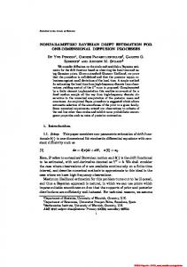
Beta-Distribution • The Beta-distribution is a two-dimensional Dirichlet with two parameters α and β; for small parameter values, we see that extreme solutions are favored
39
Noisy Observations
40
Noisy Observations • Now we want to make the model slightly more complex; we assume that we cannot observe the results of the tosses Θ directly but only (several) derived quantities (e.g., Mk noisy measurements) X with some P (X|Θ). Let Dk = {xk,j }j=1 be the observed measurements of the i−th toss and let P (xk,j |θk ) be the probability distribution (several unreliable persons inform you about the results of the tosses) • Again we might be interested in inferring the property of the dice by calculating P (g|D) (the probabilities of the properties of the dice) or in the probability of the actual tosses P (Θ1, . . . , ΘN |D). • This is now a problem with missing data (the Θ are missing); since it is relevant also for DP, we will we will only discuss approaches based on Gibbs sampling but we want to mention that the popular EM algorithm might also be used to obtain a point estimate of g • The next slide shows a graphical representation 41
Inference based on Markov Chain Monte Carlo Sampling • What we have learned about the model based on the data is incorporated in the predictive distribution
P (ΘN +1|D) =
X
P (Θ1, . . . , ΘN |D)P (ΘN +1|Θ1, . . . , ΘN )
θ1 ,...,θN S 1X s ) ≈ P (ΘN +1|θ1s , . . . , θN S s=1
s ∼ P (Θ , . . . , Θ |D) where (Monte Carlo approximation) θ1s , . . . , θN 1 N
• In contrast to before, we now need to generate samples from the posterior distribution; ideally, one would generate samples independently, which is often infeasible • In Markov chain Monte Carlo (MCMC), the next generated sample is only dependent on the previously generated sample (in the following we drop the s label in θs) 42
Gibbs Sampling • Gibbs sampling is a specific form of an MCMC process • In Gibbs sampling we initialize all variables in some appropriate way, and replace a value Θk = θk by a sample of P (Θk |{Θi = θi}i6=k , D). One continuous to do this repeatedly for all k. Note, that Θk is dependent on its data Dk = {xk,j }j but is independent of the remaining data given the samples of the other Θ • The generated samples are from the correct distribution (after a burn in phase); a problem is that subsequent samples are not independent, which would be a desired property; it is said that the chain does not mix well • Note that we can integrate out g so we never have to sample from g; this form of sampling is called collapsed Gibbs sampling
43
Gibbs Sampling (2) • We obtain (note, that Nl are the counts without considering Θk ) P (Θk = θl |{Θi = θi}i6=k , D) = P (Θk = θl |{Θi = θi}i6=k , Dk )
=
1 P (Θk = θl |{Θi = θi}i6=k )P (Dk |Θk = θl ) C
= (C =
P
l (α0 αl
1 (α0αl + Nl )P (Dk |Θk = θl ) C
+ Nl )P (Dk |Θk = θl ))
44
Auxiliary Variables, Blocked Sampling and the Standard Mixture Model
45
Introducing an Auxiliary Variable Z • The figure shows a slightly modified model; here the auxiliary variables Z have been introduced with states z 1, . . . , z r . • We have
P (Z = z k |g) = gk ,
k = 1, . . . , r
P (Θ = θj |Z = z k ) = δj,k ,
k = 1, . . . , r
• If the θ are fixed, this leads to the same probabilities as in the previous model and we can again use Gibbs sampling
46
Collapsing and Blocking • So far we had used a collapsed Gibbs sampler, which means that we never explicitly sampled from g • This is very elegant but has the problem that the Gibbs sampler does not mix very well • One often obtains better sampling by using a non-collapsed Gibbs sample, i.e., by sampling explicitly from g • The advantage is that given g, one can independently sample from the auxiliary variables in a block (thus the term blocked Gibbs sampler)
47
The Blocked Gibbs Sampler One iterates
• We generate samples from Zk |g, Dk for k = 1 . . . , N • We generate a sample from
g|Z1, . . . , ZN ∼ Dir(α∗1 + N1, . . . , α∗1 + Nr ) where Nk is the number of times that Zk = z k in the current sample.
48
Relationship to a standard Mixture Model: Learning θ • We can now relate our model to a standard mixture model; note, that this is not the same model any more • The main difference is that now we treat the the θk as random variables; this corresponds to the situation where Z would tell us which side of the dice is up and θk would correspond to a value associated with the k−th face • We now need to put a prior on θk with hyperparameters h and learn θk from data (see figure)! • A reasonable prior for the probabilities might P (π |α0) = Dir(·|α0/r, . . . , α0/r) • As a special case: when Mk = 1, and typically r