Nonparametric Bayesian Clustering Ensembles

Nonparametric Bayesian Clustering Ensembles Pu Wang1 , Carlotta Domeniconi1 , and Kathryn Blackmond Laskey2 1

2

Department of Computer Science Department of Systems Engineering and Operations Research George Mason University 4400 University Drive, Fairfax, VA 22030 USA

Abstract. Forming consensus clusters from multiple input clusterings can improve accuracy and robustness. Current clustering ensemble methods require specifying the number of consensus clusters. A poor choice can lead to under or over fitting. This paper proposes a nonparametric Bayesian clustering ensemble (NBCE) method, which can discover the number of clusters in the consensus clustering. Three inference methods are considered: collapsed Gibbs sampling, variational Bayesian inference, and collapsed variational Bayesian inference. Comparison of NBCE with several other algorithms demonstrates its versatility and superior stability.

1

Introduction

Clustering ensemble methods operate on the output of a set of base clustering algorithms to form a consensus clustering. Clustering ensemble methods tend to produce more robust and stable clusterings than the individual solutions [28]. Since these methods require only the base clustering results and not the raw data themselves, clustering ensembles provide a convenient approach to privacy preservation and knowledge reuse [31]. Such desirable aspects have generated intense interest in cluster ensemble methods. A variety of approaches have been proposed to address the clustering ensemble problem. Our focus is on statistically oriented approaches. Topchy et al. [28] proposed a mixture-membership model for clustering ensembles. Wang et al. [31] applied a Bayesian approach to discovering clustering ensembles. The Bayesian clustering ensemble model has several desirable properties [31]: it can be adapted to handle missing values in the base clusterings; it can handle the requirement that the base clusterings reside on a distributed collection of hosts; and it can deal with partitioned base clusterings in which different partitions reside in different locations. Other clustering ensemble algorithms, such as the cluster-based similarity partitioning algorithm (CSPA) [25], the hypergraph partitioning algorithm (HGPA) [25], or k-means based algorithms [18] can handle one or two of these cases; however, none except the Bayesian method can address them all. Most clustering ensemble methods have the disadvantage that the number of clusters in the consensus clustering must be specified a priori. A poor choice

2

Pu Wang, Carlotta Domeniconi, and Kathryn Blackmond Laskey

can lead to under- or over-fitting. Our approach, nonparametric Bayesian clustering ensembles (NBCE), can discover the number of clusters in the consensus clustering from the observations. Because it is also a Bayesian approach, NBCE inherits the desirable properties of the Bayesian clustering ensembles model [31]. Similar to the mixture modeling approach [28] and the Bayesian approach [31], NBCE treats all base clustering results for each object as a feature vector with discrete feature values, and learns a mixed-membership model from this feature representation. The NBCE model is adapted from the Dirichlet Process Mixture (DPM) model [22]. The following sections show how the DPM model can be adapted to the clustering ensemble problem, and examine three inference methods: collapsed Gibbs sampling, standard variational Bayesian inference, and collapsed variational Bayesian inference. These methods are compared in theory and practice. Our empirical evaluation demonstrates the versatility and superior stability and accuracy of NBCE.

2

Related Work

A clustering ensemble technique is characterized by two components: the mechanism to generate diverse partitions, and the consensus function to combine the input partitions into a final clustering. Diverse partitions are typically generated by using different clustering algorithms [1], or by applying a single algorithm with different parameter settings [10, 16, 17], possibly in combination with data or feature sampling [30, 9, 20, 29]. One popular methodology to build a consensus function utilizes a coassociation matrix [10, 1, 20, 30]. Such a matrix can be seen as a similarity matrix, and thus can be used with any clustering algorithm that operates directly on similarities [30, 1]. As an alternative to the co-association matrix, voting procedures have been considered to build consensus functions in [7]. Gondek et al. [11] derive a consensus function based on the Information Bottleneck principle: the mutual information between the consensus clustering and the individual input clusterings is maximized directly, without requiring approximation. A different popular mechanism for constructing a consensus maps the problem onto a graph-based partitioning setting [25, 3, 12]. In particular, Strehl et al. [25] propose three graph-based approaches: Cluster-based Similarity Partitioning Algorithm (CSPA), HyperGraph Partitioning Algorithm (HGPA), and Meta-Clustering Algorithm (MCLA). The methods use METIS (or HMETIS) [15] to perform graph partitioning. The authors in [23] develop soft versions of CSPA, HGPA, and MCLA which can combine soft partitionings of data. Another class of clustering ensemble algorithms is based on probabilistic mixture models [28, 31]. Topchy et al. [28] model the clustering ensemble as a finite mixture of multinomial distributions in the space of base clusterings. A consensus result is found as a solution to the corresponding maximum likelihood problem using the EM algorithm. Wang et al. [31] proposed Bayesian Cluster Ensembles (BCE), a model that applies a Bayesian approach to protect against

Nonparametric Bayesian Clustering Ensembles

3

the over-fitting to which the maximum likelihood method is prone [28]. The BCE model is applicable to some important variants of the basic clustering ensemble problem, including clustering ensembles with missing values, as well as row-distributed or column-distributed clustering ensembles. Our work extends the BCE model to a nonparametric version, keeping all the advantages thereof, while allowing the number of clusters to adapt to the data.

3

Dirichlet Process Mixture Model

The Dirichlet process (DP) [8] is an infinite-dimensional generalization of the Dirichlet distribution. Formally, let S be a set, G0 a measure on S, and α0 a positive real number. The random probability distribution G on S is distributed according to DP with the concentration parameter α0 and the base measure G0 , if for any finite partition {Bk }1≤k≤K of S: (G(B1 ), G(B2 ), · · · , G(BK )) ∼

Dir(α0 G0 (B1 ), α0 G0 (B2 ), · · · , α0 G0 (BK )) Let G be a sample drawn from a DP. Then with probability 1, G is a discrete distribution [8]. In addition, if the first N −1 draws from G yield K distinct values ∗ θ1:K with multiplicities n1:K , then the probability of the N th draw conditioned on the previous N − 1 draws is given by the P´olya urn scheme [5]: ( θN =

θk∗ , ∗ ∼ G0 , θK+1

with prob with prob

nk , N −1+α0 α0 N −1+α0

k ∈ {1, · · · , K}

The DP is often used as a nonparametric prior in Bayesian mixture models [2]. Assume the data are generated from the following generative procedure: G ∼ Dir(α0 , G0 ) θ1:N ∼ G N Y x1:N ∼ F (·|θn ) n=1

The θ1:N typically contains duplicates; thus, some data points are generated from the same mixture component. It is natural to define a cluster as those observations generated from a given mixture component. This model is known as the Dirichlet process mixture (DPM) model. Although any finite sample contains only finitely many clusters, there is no bound on the number of clusters and any new data point has non-zero probability of being drawn from a new cluster [22]. Therefore, DPM is known as an “infinite” mixture model. The DP can be generated via the stick-breaking construction [24]. Stickbreaking draws two infinite sequences of independent random variables, vk ∼

4

Pu Wang, Carlotta Domeniconi, and Kathryn Blackmond Laskey

Beta(1, α0 ) and θk∗ ∼ G0 for k = {1, 2, · · · }. Let G be defined as: k−1 Y

π k = vk

(1 − vj )

(1)

πk δ(θ, θk∗ )

(2)

j=1

G(θ) =

∞ X k=1

where π = hπk |k = 1, 2, · · · i are the mixing proportions of the infinite number of components. Then G ∼ Dir(α0 , G0 ). It is helpful to use an indicator variable zn to denote which mixture component is associated with xn . The generative procedure for the DPM model using the stick-breaking construction becomes: 1. Draw vk ∼ Beta(1, α0 ), k = {1, 2, · · · } and calculate π as in Eq (1). 2. Draw θk∗ ∼ G0 , k = {1, 2, · · · } 3. For each data point: – Draw zn ∼ Discrete(π) – Draw xn ∼ F (·|θz∗n ) In practice, the process is typically truncated at level K by setting vK−1 = 1 [13]; Eq (1) then implies that all πk for k > K are zero. The truncated process is called truncated stick-breaking (TSB). The resulting distribution, the truncated Dirichlet process (TDP), closely approximates the Dirichlet process when K is sufficiently large. The choice of the truncation level K is discussed in [13]. The joint probability over data items X = hxn |n ∈ {1, · · · , N }i, component assignments Z = hzn |n ∈ {1, · · · , N }i, stick-breaking weights v = hvk |k ∈ {1, · · · , K}i and component parameters θ ∗ = hθk∗ |k ∈ {1, · · · , K}i is: " ∗

p(X, Z, v, θ ) =

N Y

#" F (xn |θz∗n )πzn (v))

n=1

K Y

# G0 (θk∗ )Beta(vk ; 1, α0 )

k=1

Another approach to approximate the DP is to assume a finite but large Kdimensional symmetric Dirichlet prior (FSD) on the mixture proportion π [14], which is π ∼ Dir(α0 /K, · · · , α0 /K). This results in the joint distribution: p(X, Z, π, θ ∗ ) =

"

N Y n=1

#" F (xn |θz∗n )πzn

K Y

# G0 (θk∗ )

k=1

Dir(π;

α0 α0 ,··· , ) K K

With TSB, the cluster weights differ in expected value, with lower-numbered cluster indices having higher probability. With FSD, the clusters are exchangeable. A detailed comparison of these DP approximations can be found in [19].

4

NBCE Generative Model

Following [28] and [31], we assume there are M base clustering algorithms, each generating a hard partition on the N data items to be clustered. Let Jm denote

Nonparametric Bayesian Clustering Ensembles

5

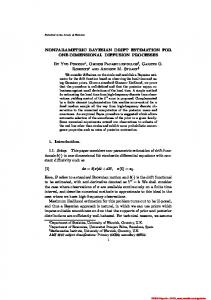
the number of clusters generated by the mth clustering ϕm , m ∈ {1, · · · , M }, and let ynm ∈ {1, · · · , Jm } denote the cluster ID assigned to the nth data item xn by ϕm , n ∈ {1, · · · , N }. The row y n = hynm |m ∈ {1, · · · , M }i of the base clustering matrix Y gives a new feature vector representation for the nth data item. Figure 1 depicts the generative model for Y . We assume y n is generated from a truncated Dirichlet Process mixture model, where α0 is the concentration parameter, G0 is the base measure, and K is the truncation level. The probability of generating a cluster ID ynm = jm by ϕm for xn is θnmjm , jm ∈ {1, · · · , Jm } PJm and jm =1 θnmjm = 1. So y n = hynm = jm |m ∈ {1, · · · , M }i is generated QM with probability m=1 θnmjm . We define θ nm = hθnmjm |jm ∈ {1, · · · , Jm }i. We (m) (m) further assume a prior G0 for θ ·m = {θ nm |n = 1, · · · , N }, where G0 is a symmetric Dirichlet distribution of dimension Jm with hyperparameter β. The (1) (M ) base measure G0 is defined as G0 = G0 ×· · ·×G0 . We denote θ n = hθ nm |m ∈ {1, · · · , M }i. Since the truncation level is K, there are K unique θ n , denoted ∗ as θ ∗k = hθ ∗km |m ∈ {1, · · · , M }i, where θ ∗km = hθkmj |jm ∈ {1, · · · , Jm }i, m PJm ∗ jm =1 θkmjm = 1 and k ∈ {1, · · · , K}. We associate with each xn an indicator variable zn to indicate which θ ∗k is assigned to xn ; if zn = k, then θ n = θ ∗k . A consensus cluster is defined as a set of data items associated with the same θ ∗k . That is, zn indicates which consensus cluster xn belongs to. There are at most K consensus clusters, but some consensus clusters may be empty; we define the total number of consensus clusters to be the number of distinct zn in the sample.

α0

G

(m)

G0

∗ θ!km

!π

K

zn N

ynm M

Fig. 1. Nonparametric Bayesian Clustering Ensembles Model

The stick breaking generative process for Y is: 1. Draw vk ∼ Beta(1, α0 ), for k = {1, · · · , K} and calculate π as in Eq (1) 2. Draw θ ∗k ∼ G0 , for k = {1, · · · , K} 3. For each xn : – Draw zn ∼ Discrete(π) – For each base clustering ϕm , draw ynm ∼ Discrete(θ ∗zn m )

6

Pu Wang, Carlotta Domeniconi, and Kathryn Blackmond Laskey

Using the symmetric Dirichlet prior, step 1 becomes: 1. Draw π ∼ Dir( αK0 , · · · , αK0 )

5

Inference and Learning

This section considers three inference and learning methods: collapsed Gibbs sampling, standard variational Bayesian, and collapsed variational Bayesian inference. Table 1 gives the notation used throughout this section. The joint probability of observed base clustering results Y = hy n |n ∈ {1, · · · , N }i, indicator variables Z = hzn |n ∈ {1, · · · , N }i, component weights π = hπk |k ∈ {1, · · · , K}i, and component parameters θ ∗ = hθ ∗k |k ∈ {1, · · · , K}i is given by: p(Y , Z, π, θ ∗ |α0 , G0 ) = N Y

! ∗

p(zn |π)p(y n |θ , zn )

· p(π|α0 )

n=1 N Y

K Y

! p(θ ∗k |G0 )

=

k=1

p(zn |π)

n=1

M Y

! p(ynm |θ ∗zn m )

· p(π|α0 )

m=1

K Y M Y k=1 m=1

(m) p(θ ∗km |G0 )

! (3)

After marginalizing out the parameters π and θ, the complete data likelihood is: (4)

p(Y , Z|α0 , G0 , ) = p(Z|α0 )

 ·

M Y

K Y

m=1 k=1

Γ (Jm β) Γ (Jm β + Nz· =k ) j

Jm Y m



=jm Nzy··m ) =k 

Γ (β + Γ (β) =1

where for the two DP approximations, p(Z|α0 ) is different [19]: Y Γ (1 + Nz =k )Γ (α0 + Nz >k ) · · pT SB (Z|α0 ) = Γ (1 + α0 + Nz· ≥k ) kh ¬n 1 + α0 + Nz¬n 1 + α + N 0 ≥k z· ≥h · α0 K

+ Nz¬n · =k pF SD (zn = k|Z ¬n ) = α0 + N − 1 5.2

hh · ≥h h