and Control (CDC), pages 1207â1213, 2012. [4] Marc Peter Deisenroth and Carl Edward Rasmussen. .... [36] Peter Whittle. Risk-Sensitive Linear/Quadratic/ ...
DIRTREL: Robust Trajectory Optimization with Ellipsoidal Disturbances and LQR Feedback Zachary Manchester and Scott Kuindersma School of Engineering and Applied Sciences Harvard University Cambridge, MA 02138 Email: {zmanchester, scottk}@seas.harvard.edu
Abstract—Many critical robotics applications require robustness to disturbances arising from unplanned forces, state uncertainty, and model errors. Motion planning algorithms that explicitly reason about robustness require a coupling of trajectory optimization and feedback design, where the system’s closedloop response to bounded disturbances is optimized. Due to the often-heavy computational demands of solving such problems, the practical application of robust trajectory optimization in robotics has so far been limited. We derive a tractable robust optimization algorithm that combines direct transcription with linear-quadratic control design to reason about closed-loop responses to disturbances. In the case of ellipsoidal disturbance sets, the state and input deviations along a nominal trajectory can be computed locally in closed form, thus allowing for fast evaluations of robust cost and constraint functions. The resulting algorithm, called DIRTREL, is an extension of classical direct transcription that demonstrably improves tracking performance over non-robust formulations while incurring only a modest increase in computational cost. We evaluate the algorithm in several simulated robot control tasks.
I. I NTRODUCTION Motion planning has been an active research topic that has yielded several successes in recent years, from samplingbased algorithms that scale to large state spaces [13, 14] to nonlinear optimization methods capable of handling complex dynamic constraints [32, 33, 2] and contacts [34, 30, 31]. Despite this, the world’s most advanced robots still struggle to perform robustly when subjected to disturbances caused by unplanned forces, state estimation errors, and model inaccuracies. Algorithms that explicitly reason about robustness require a coupling of motion planning and feedback design, frequently resulting in computationally expensive algorithms that have limited practical utility in robotics. This paper aims to address this problem by extending a popular class of trajectory optimization methods to optimize the closed-loop performance of the system near the nominal trajectory. This paper builds on previous work on robust motion planning based on direct trajectory optimization [26, 3] and differential dynamic programming (DDP) [27, 6, 29]. Robust motion planning algorithms often differ in the precise notion of robustness that they seek to optimize. For example, deterministic minimax methods optimize performance against worst-case disturbances, while stochastic risk-sensitive methods optimize cost functionals that account for variance in performance. To date, we are unaware of any approach that has resulted in
an algorithm that can simultaneously capture bounded disturbances that enter the system dynamics nonlinearly, handle nonlinear state and input constraints, and scale to practical robotic systems with high dimensional state and input spaces. We propose a robust motion planning algorithm that reasons about disturbances by optimizing a robust cost function that is differentiable and can be computed analytically. The key to our approach is the observation that, by restricting the problem to time-varying linear feedback (e.g., LQR) and ellipsoidal disturbance sets, bounds on state and input deviations can be computed locally along a nominal trajectory in closed form. As a result, a tractable penalty function over the set of all disturbances can be defined and constraints on the perturbed states and inputs can be enforced. We incorporate this robust penalty function into a direct transcription method (DIRTRAN), thereby inheriting the well-known benefits of these algorithms (easy handling of constraints, good numerical conditioning, and sparsity). The resulting algorithm, called DIRTREL (DIRect TRanscription with Ellipsoidal disturbances and Linear feedback), can be applied to the same class of systems as standard direct transcription, while significantly improving tracking performance of the resulting plans in the presence of disturbances. This paper is organized as follows. In Section II we summarize prior work related to robust control in robotics. We then review the classic direct transcription algorithm in Section III before proposing our robust extension, DIRTREL, in Section IV. Section V describes several simulation experiments used to validate our new algorithm and analyze its computational performance. Finally, we discuss conclusions and future work in Section VI. II. R ELATED W ORK The theory of robust control of linear dynamical systems has developed into a rich literature over the past four decades [38]. In particular, a set of techniques collectively known as H∞ control allows designers to optimize performance in the presence of disturbances by minimizing the L2 gain of the closedloop system. H∞ techniques have also been investigated for nonlinear systems [17, 19] and 6-DoF flexible manipulator tracking [37], but these algorithms do not scale gracefully to many problems of interest in robotics.
Several robust variants of differential dynamic programming [11] have been proposed for solving worst-case minimax problems [27], risk-sensitive optimizations for stochastic systems [6], and cooperative stochastic games [29]. Like the algorithm proposed in this paper, these methods consider system responses under linear feedback, but they use different robustness metrics and lack the ability to explicitly incorporate bounds on disturbances. State and input constraints require additional care, but could be handled approximately using penalty functions or exactly using augmented Lagrangian or quadratic programming approaches [16]. In contrast, the algorithm presented in this paper naturally handles nonlinear constraints on the nominal and disturbed state and input trajectories. Tube-based model-predictive control (MPC) algorithms [22] use MPC to reject additive disturbances along an optimized nominal trajectory. Mordatch et al. [26] developed an ensemble trajectory optimization method that aims to reduce the expected cost under random model parameters while reducing trajectory variation under PD control. Lou and Hauser [18] combined robust motion planning with model estimation to optimize robust motions involving contact changes. However, their approach required a kinematic plan to be given and only optimized the timing of the motion. Several authors have developed risk-sensitive optimal control methods [10, 36] for nonlinear stochastic systems with known models [6] or datadriven control-learning approaches [35, 4, 15]. Verification approaches to feedback motion planning attempt to compute regions of finite-time invariance, or “funnels,” which provide a certificate of stability. Moore et al. extended the LQR-Trees framework to include uncertainty in funnel estimates using a Common Lyapunov formulation of a sums-of-squares (SOS) program [25]. A related line of work led to the development of robust adaptive tracking controllers with guaranteed finite-time performance [24]. Majumdar and Tedrake extended these ideas to support robust online planning using pre-planned funnel libraries to construct a policy that can adjust funnels and tracking controllers based on sensor feedback [20]. The algorithm we describe is complementary to these methods in that it aims to design robust trajectories, not verify (or switch between) pre-computed trajectories. Griffin and Grizzle [8] and Dai and Tedrake [3] augment direct trajectory optimization methods with cost functionals that weight the tracking performance of linear feedback controllers. However, there are several important differences from our approach. In [8], a fixed-gain proportional-integral controller is assumed, placing potentially significant limits on closed-loop performance. In [3], the elements of the timevarying cost-to-go matrix associated with an LQR tracking controller are added as decision variables to the optimization problem, and disturbances are handled through a sampling scheme that scales poorly with the dimensionality of the disturbance vector. These design choices substantially increase the size and complexity of the nonlinear program that must be solved, limiting the algorithm’s applicability to complex robot planning problems.
III. D IRECT T RANSCRIPTION Direct transcription methods solve optimal control problems by explicitly parameterizing the state and control trajectories and formulating a large, sparse nonlinear program [1]. Compared to shooting methods, these algorithms enable straightforward inclusion of state constraints and avoid numerical pitfalls such as the “tail wagging the dog” effect, at the expense of a larger problem size. The resulting nonlinear optimization problems can be solved using commercial sequential-quadratic programming (SQP) packages, such as SNOPT [7], that exploit the sparsity patterns in the linearized constraint matrix. Given a nonlinear dynamical system, x˙ = f (x, u), we discretize the system trajectory in time using N knot points, x1:N = {x1 , . . . , xN } and u1:N −1 = {u1 , . . . , uN −1 }, and solve the following NLP, minimize
x1:N , u1:N −1 , h
gN (xN ) +
N −1 X
g(xi , ui )
i=1
subject to xi+1 = xi + f (xi , ui ) · h
∀i = 1 : N − 1
ui ∈ U
∀i = 1 : N − 1
xi ∈ X
∀i = 1 : N
(1)
hmin ≤ h ≤ hmax where g(·, ·) and gN (·) are cost functions, X is a set of feasible states, U is a set of feasible inputs, and h is the time step used for integration. For simplicity, we have assumed a forward Euler integration scheme, although other schemes such as backward Euler or midpoint interpolation can be used instead. By including h as a decision variable, we allow the solver to scale the duration of the trajectory. In what follows, we write the discrete-time dynamics as an iterated map, xi+1 = fh (xi , ui ), for conciseness. IV. D IRECT T RANSCRIPTION WITH E LLIPSOIDAL D ISTURBANCES The following subsections describe how we extend the standard DIRTRAN problem to incorporate linear feedback, bounded disturbances, and a cost function that penalizes closed-loop deviations from the nominal trajectory. A. State and Input Deviations First, we assume disturbances, wi ∈ W, can enter into the dynamics in a general nonlinear way: xi+1 = fh (xi , ui , wi ).
(2)
Under this definition, wi could, for example, correspond to model parameter uncertainty, unplanned external forces, or state estimation errors. A trajectory, x1:N , u1:N −1 , that satisfies xi+1 = fh (xi , ui , 0) (3) is referred to as a nominal trajectory. Given a disturbance sequence, w1:N −1 , the deviations from the nominal state trajectory are calculated as δxi+1 = fh (xi + δxi , ui + δui , wi ) − xi+1 ,
(4)
and we assume that deviations from the nominal input sequence are computed using a linear feedback controller, δui = −Ki δxi .
(5)
Any reasonable choice of linear controller can be used, but in the development that follows we define Ki to be the optimal time-varying linear quadratic regulator (TVLQR) gain matrix computed by linearizing the dynamics along the nominal trajectory and solving the dynamic Riccati equation, Ki
=
(R + BiT Pi+1 Bi )−1 (BiT Pi+1 Ai )
Pi−1
=
Q + ATi Pi Ai
step i can be computed. As in equation (7), we parameterize these ellipsoids by matrices Ei � 0. Assuming a bound on the initial state deviation δx1 parameterized by E1 , the matrices Ei can be found at all future time steps using the system dynamics. Linearizing equation (4) about the nominal trajectory gives a set of linear time-varying equations of the form δxi+1 ≈ Ai δxi + Bi δui + Gi w ,
where Gi = ∂fh /∂w|xi ,ui ,0 . A recursion for Ei+1 in terms of Ei and D can then be defined:
−ATi Pi Bi (R + BiT Pi Bi )−1 (BiT Pi Ai ) , where Ai = ∂fh /∂x|xi ,ui ,0 , Bi = ∂fh /∂u|xi ,ui ,0 , PN ≡ QN , and Q, QN � 0 and R � 0 are state and input cost matrices. B. A Robust Cost Function To optimize robustness, our approach augments the NLP (1) with an additional cost term, `W (x1:N , u1:N −1 ). Intuitively, we want this function to penalize deviations of the closedloop system from the nominal trajectory in the presence of disturbances, wi , drawn from the set W. To penalize these deviations, we assume a quadratic one-step cost, δxTi Q` δxi + δuTi R` δui , where Q` � 0 and R` � 0 are positive semidefinite cost matrices. In order to compute δx1:N and δu1:N −1 , we need a welldefined disturbance sequence, w1:N −1 . Instead of resorting to sampling or worst-case minimax optimization methods, we instead approximate the robust cost averaged over the entire disturbance set and summed along the trajectory: 1 `W (x1:N , u1:N −1 ) ≈ Vol(W) +
N −1 X
Z W
δxTN Q`N δxN !
δxTi Q` δxi
+
δuTi R` δui
�
(8)
dW. (6)
i=1
For general nonlinear systems and disturbance sets, the integral in equation (6) cannot be easily computed. However, the assumption of an ellipsoidal disturbance set and a linearization of the dynamics about the nominal trajectory leads to a computationally tractable approximation. While linearization of the dynamics may seem limiting, we argue that the resulting local approximation has roughly the same region of validity as the LQR tracking controller. It therefore does not impose significant practical limitations beyond those already associated with the use of linear feedback. We parameterize the ellipsoidal set W by a matrix D � 0, such that wT D−1 w ≤ 1. (7) Note that the set of vectors describing the semi-axes of W are given by the columns of the principal square root of D, defined such that D = D1/2 D1/2 . Using the fact that ellipsoids map to ellipsoids under linear transformations, approximate ellipsoidal bounds on the state deviations, δxi , at each time
Mi+1 = Fi Mi FiT , where Mi and Fi are defined as follows, � � Ei Hi Mi = HiT D Fi =
� � (Ai − Bi Ki ) Gi , 0 I
(9)
(10)
(11)
and M1 is initialized with H1 = 0 and E1 � 0. The propagation of Ei forward in time through the linearized dynamics bears some resemblance to the covariance propagation step in a Kalman Filter. However, there are some important differences. First, as a matter of interpretation, equation (9) is purely deterministic; Ei represents a strict bound rather than a statistical covariance. Second, equations (9)–(11) contain additional cross terms, signified by the presence of the Hi blocks in the matrix Mi , which are absent in the Kalman Filter due to the statistical independence of noise at different time steps. Returning to the cost function `W (x1:N , u1:N −1 ), we replace the volume integral over the disturbance set in equation 1/2 (6) with a sample mean calculated over the columns of Ei , which correspond to the semi-axis vectors of the ellipsoids bounding the state, `W (x1:N , u1:N −1 ) = N −1 1 X + nx i=1
1 nx
X
δxTN Q`N δxN
1/2 δxN ∈col(EN )
X
δxTi Q` δxi + δuTi R` δui , (12) 1/2
δxi ∈col(Ei
)
where nx is the state dimension. In the remainder of the paper we omit this constant factor, as it has no effect on the results and can be folded into the cost-weighting matrices. 1/2 The sum over the columns of Ei can be computed by rewriting the quadratic forms in equation (6) using the trace operator, δxTi Qδxi = Tr(Q δxi δxTi )
(13)
δuTi Rδui = Tr(R δui δuTi ),
(14)
and replacing the outer products δxi δxTi and δui δuTi with suitable expressions involving Ei :
minimize
`W (x1:N , u1:N −1 ) = Tr (QN EN ) +
can be expressed as the following NLP:
x1:N , u1:N −1 , h N −1 X
� Tr (Q + KiT RKi )Ei . (15)
i=1
Equations (9)–(11) and (15) provide an easily computable cost function that quantifies the system’s closed-loop sensitivity to disturbances. The evaluation of `W (x1:N , u1:N −1 ) is summarized in Algorithm 1. Algorithm 1 Robust Cost Function 1: function `W (x1:N , u1:N −1 , D, E1 , Q` , R` , Q`N , Q, R) 2: for i = 1 . . . N − 1 do 3: Ai ← ∂x=xi fh (x, u, w) 4: Bi ← ∂u=ui fh (x, u, w) 5: Gi ← ∂w=0 fh (x, u, w) 6: end for 7: K1:N −1 ← T V LQR(A1:N −1 , B1:N −1 , Q, R) 8: H1 ← 0 9: for i = 1 . . . N − 1 do � 10: ` ← ` + Tr (Q` + KiT R` Ki )Ei 11: Ei+1 ← (Ai − Bi Ki )Ei (Ai − Bi Ki )T + (Ai − Bi Ki )Hi GTi + Gi H T (Ai − Bi Ki )T + Gi DGTi 12: Hi+1 = (Ai − Bi Ki )Hi + Gi D 13: end for � 14: ` ← ` + Tr Q`N EN 15: return ` 16: end function
C. The DIRTREL Algorithm We now develop a complete algorithm that outputs a feasible trajectory and feedback controller for the nominal (w = 0) system such that the sensitivity of the closed-loop system to disturbances is minimized. In addition to augmenting (1) with `W (x1:N , u1:N −1 ), we must also ensure that the closed-loop system obeys state and input constraints. To do so, we again 1/2 use the columns of Ei , which give the extreme values of δxi on the boundary of the ellipsoid. In particular, all state constraints on the nominal trajectory must also be applied to the set of disturbed state vectors, � � 1/2 xW , (16) i = xi ± col Ei and all input constraints must also be applied to the set of disturbed closed-loop inputs, � � T 1/2 uW . (17) i = ui ± col (Ki Ei Ki ) The resulting optimization problem, referred to as DIRTREL,
`W (x1:N , u1:N −1 ) + gN (xN ) +
N −1 X
g(xi , ui )
i=1
subject to xi+1 = fh (xi , ui )
∀i = 1 : N − 1
ui ∈ U
∀i = 1 : N − 1
uW i
∀i = 1 : N − 1
∈U
xi ∈ X
∀i = 1 : N
xW i ∈X
∀i = 1 : N
(18)
hmin ≤ h ≤ hmax Unlike minimax approaches to robust control, `W (x1:N , u1:N −1 ) and the associated robust state and input constraints in (18) are smooth functions of the state and input trajectories. As a result, they can be differentiated in closed form and good convergence behavior can be achieved with standard NLP solvers based on Newton’s method [28]. Also, since DIRTREL builds on the classic DIRTRAN algorithm, it inherits the property that its computational complexity scales linearly with the number of knot points [1]. In addition, we note that the number of decision variables has remained the same as standard DIRTRAN. The computation of the LQR Riccati recursion and the derivatives of `W requires computation polynomial in the number of states. V. E XAMPLES We now present several examples to demonstrate the performance of DIRTREL. Comparisons are made to the standard approach of performing trajectory optimization with DIRTRAN followed by synthesis of a time-varying LQR tracking controller. All algorithms are implemented in MATLAB, and the commercial SQP solver SNOPT [7] is used to solve the resulting NLPs. DIRTREL’s running time on all examples is between two and four times that of standard DIRTRAN. Empirically, the increased running time is primarily attributed to the calculation of derivatives of the robust cost function (currently done in MATLAB). We anticipate substantial gains could be achieved with a more careful C++ implementation. A. Pendulum with Uncertain Mass In the first test case, a simple pendulum of unit length with an input torque is considered. The mass of the pendulum is bounded between 0.8 and 1.2, and the actuator has torque limits −3 ≤ u ≤ 3. The goal is to swing the pendulum from its downward stable equilibrium at θ = 0 to the upward unstable equilibrium at θ = π in minimum time. The following cost-weighting matrices are used in both the robust cost function `W and the LQR tracking controller: R = R` = 0.1 � � 10 0 Q = Q` = 0 1 � � 100 0 ` QN = QN = . 0 100
mp
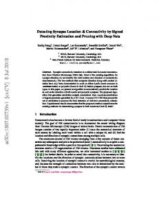
The matrix D corresponding to the ±0.2 bound on the pendulum mass is D = (0.2)2 , and the algorithm is initialized with no initial disturbance on the state: � � 0 0 E1 = . (19) 0 0 The state and input trajectories produced by DIRTRAN and DIRTREL are shown in Figure 1. Consistent with the minimum-time nature of the problem, DIRTRAN generates a bang-bang control policy that uses the maximum torque that the actuator is capable of producing. DIRTREL, on the other hand, produces a nominal trajectory that stays clear of the torque limits. Over several numerical simulations, the DIRTREL controller was able to perform successful swingups of pendulums with mass values up to m ≈ 1.3, while the DIRTRAN controller was successful only up to m ≈ 1.1. While tuning the cost function used in DIRTRAN through trial and error could likely result in more robust tracking performance, DIRTREL allows known bounds on the plant model to be incorporated in a principled and straight-forward manner that eliminates the need for such “hand tuning.”
θ
2 0
DIRTREL DIRTRAN
−2
l
mc ✓
x Fig. 2.
u, Fc
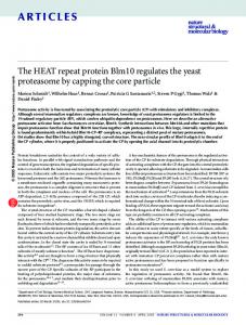
The Cart Pole system with unmodeled friction with the ground.
is l = 0.5. The cart’s actuator is limited to −10 ≤ u ≤ 10. The nominal model used during trajectory optimization has no friction, while in simulation the following friction force is applied to the cart, Fc = − sign(x)µF ˙ N,
(20)
where µ is a friction coefficient and FN is the normal force exerted between the cart and the ground. To account for unmodeled friction in DIRTREL, we make w an exogenous force input to the cart and bound it such that −2 ≤ w ≤ 2, corresponding to D = 4. We use the following running cost in both DIRTRAN and DIRTREL: g(xi , ui ) = xTi xi + 0.1u2i ,
0
0.5
1
1.5
2
2.5
2 u
g
0 −2 0
0.5 Fig. 1.
1 1.5 Time (s)
2
2.5
Pendulum swing-up trajectories
B. Cart Pole with Unmodeled Friction Motivated by the fact that friction is often difficult to model accurately in mechanical systems, we considered a swing-up problem for the cart pole system (Figure 2) with unmodeled friction. The system’s state vector x ∈ R4 consists of the cart’s position, the pendulum angle, and their corresponding first derivatives. The input u ∈ R consists of a force applied to the cart. Nonlinear Coulomb friction is applied between the cart and the ground. Once again, the goal is to swing the pendulum from the downward θ = 0 position to the upward θ = π position. In our simulations, the cart mass is taken to be mc = 1, the pendulum mass is mp = 0.2, and the pendulum length
and a terminal constraint is enforced on the final state, xN = [0 π 0 0]T . The following cost-weighting matrices are used in both the robust cost function `W and the LQR tracking controller: R = R` = 1 10 0 Q = Q` = 0 0 100 0 ` QN = QN = 0 0
0 0 0 10 0 0 0 1 0 0 0 1 0 100 0 0
0 0 100 0
0 0 . 0 100
Figure 3 shows the nominal trajectories generated by both DIRTRAN and DIRTREL. As in the pendulum example, the DIRTREL trajectory avoids saturating the actuator while taking longer to complete the swing up. In this case, however, the two trajectories are qualitatively different; the DIRTREL trajectory takes one additional swing to reach the vertical position. Numerous simulations were performed while varying the friction coefficient µ to characterize the robustness of the closed-loop systems. Successful swing up was observed using the DIRTRAN trajectory with LQR tracking over the range 0 ≤ µ ≤ 0.064, while the DIRTREL trajectory with LQR tracking was successful over the range 0 ≤ µ ≤ 0.295.
1
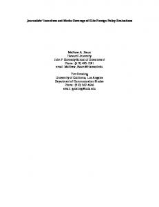
In the second trajectory (DIRTREL-2), the disturbance bounds were set to ±0.4 in the x and y axes, corresponding to, 2 .4 0 0 0 . D = 0 .42 0 0 .052
x
0.5 0 −0.5
0
1
2
3
4
5
4 θ
2 DIRTREL DIRTRAN
0 −2
0
1
2
3
4
5
0
1
2 3 Time (s)
4
5
10 u
5 0 −5 −10
Fig. 3.
Fig. 4. DIRTRAN (red), DIRTREL-1 (blue), and DIRTREL-2 (green) quadrotor trajectories.
Cart pole swing-up trajectories
C. Quadrotor with Wind Gusts Next, we demonstrate DIRTREL on a quadrotor subjected to random wind gusts. The goal is for the aircraft to move from an initial position to a final position while navigating an obstacle field. The dynamics are described using the model of [23] and wind gusts are simulated by applying band-limited white noise accelerations to the system. In both DIRTRAN and DIRTREL, constraints on the initial and terminal states of the quadrotor were applied, and a quadratic running cost of the following form was used: g(xi , ui ) = xTi Qxi + uTi Rui .
(21)
The same weighting matrices were used in the running cost, the robust cost `W , and the LQR tracking controllers: R = R` = 0.1 I4×4 � 10 I6×6 ` Q=Q = 0 � 10 I6×6 QN = Q`N = 0
0
�
I6×6 0
�
I6×6
Two different trajectories were computed with DIRTREL. In the first (DIRTREL-1), disturbances were bounded by ±0.2 in the x and y axes and ±0.05 in the z axis, corresponding to the following D matrix: 2 .2 0 0 0 . D = 0 .22 0 0 .052
Figure 4 shows the nominal trajectories generated by DIRTRAN and DIRTREL. The DIRTRAN trajectory takes the shortest path to the goal state. However, it passes quite close to several obstacles. The DIRTREL trajectories, on the other hand, take longer paths to the goal but maintain greater distances from each obstacle. We performed closed-loop simulations with random wind gusts of varying amplitudes. Disturbance inputs were generated by low-pass filtering white noise, then rescaling the resulting disturbance trajectory so that its maximum amplitude was equal to the desired value. Gust amplitudes in the x and y directions were varied from 0.1 to 0.5, while amplitudes in the z direction were held fixed at 0.05. TABLE I N UMBER OF CLOSED - LOOP QUADROTOR TRAJECTORIES WITH OBSTACLE COLLISIONS OUT OF 100 TRIALS . Max Gust 0.1 0.2 0.3 0.4 0.5
DIRTRAN 37 65 77 82 90
DIRTREL-1 0 0 3 5 9
DIRTREL-2 0 0 0 0 1
Table I shows the results of 100 trials performed at each amplitude level. As expected, no collisions occurred using the DIRTREL controllers for gust amplitudes within the bounds imposed during planning (0.2 and 0.4 for for the first and second cases, respectively) result in no collisions, while the DIRTRAN controller was unable to avoid collisions with obstacles in many trials at every amplitude level. To offer a more generous comparison, we calculated the closest distance between the quadrotor and an obstacle in the
nominal DIRTREL-2 trajectory, inflated the obstacles by that distance, and re-planned a new trajectory with DIRTRAN. Obstacle inflation (also called constraint shrinking) techniques are a heuristic approach to improve robustness using traditional planning methods. The corresponding closed-loop simulation results are shown in Table II. Due to its ability to explicitly reason about the closed-loop dynamics and how disturbances act on particular states, DIRTREL offers significantly better robustness than naive obstacle inflation. TABLE II N UMBER OF CLOSED - LOOP QUADROTOR TRAJECTORIES WITH OBSTACLE COLLISIONS OUT OF 100 TRIALS AFTER PLANNING WITH INFLATED OBSTACLES . Max Gust 0.1 0.2 0.3 0.4 0.5
DIRTRAN (INFLATED) 0 1 4 21 27
D. Robot Arm with Fluid-Filled Container Finally, we use DIRTREL to plan the motion of a robot arm carrying a fluid-filled container. The goal is to gently place the container on a shelf while avoiding collisions. A dynamics model of the seven-link Kuka IIWA arm was used, and bounds of ±3 Newtons in the x and y directions and ±10 Newtons in the z direction were placed on disturbance forces applied to the end effector in DIRTREL to account for both uncertain mass and un-modeled fluid-slosh dynamics inside the container. In both algorithms, constraints were placed on the initial and final poses of the arm. The same quadratic running cost penalizing joint torque and quadratic terminal cost penalizing the final velocity of the end effector were also applied in both algorithms. The terminal cost was intended to encourage a gentle placement of the container on the shelf. The following weighting matrices were used in both the robust cost function and LQR tracking controllers: R = R` = 0.01 I7×7 � 100 I7×7 ` Q=Q = 0 � 500 I7×7 QN = Q`N = 0
0 10 I7×7
�
� 0 . 50 I7×7
The nominal trajectories produced by DIRTRAN and DIRTREL are depicted in Figure 5. As expected, the DIRTREL trajectory takes a wider path around the obstacle. However, as in the quadrotor example, this kinematic behavior can also be reproduced with DIRTRAN by inflating the obstacle. To compare dynamic performance, we compute the RMS deviations of the closed-loop system from the nominal trajectory with each controller. Ten trials were performed while varying the mass of the container and applying band-limited white noise disturbance forces to the end effector to simulate fluid slosh. DIRTRAN achieved an RMS state deviation of
Fig. 5. Nominal end-effector trajectories produced by DIRTRAN (red) and DIRTREL (blue).
0.1192 and an RMS input deviation of 4.478, while DIRTREL achieved an RMS state deviation of 0.0735 and an RMS input deviation of 4.422. The DIRTREL controller achieved nearly 40% better closed-loop tracking performance while using roughly the same control effort as the DIRTRAN controller. VI. D ISCUSSION We have presented a new algorithm, DIRTREL, for robust feedback motion planning. By bounding disturbance sets with ellipsoids and assuming linear closed-loop feedback control, we have derived a computationally tractable robust penalty function and a method to account for state and input constraints along disturbed system trajectories. The resulting algorithm produces nominal trajectories and closed-loop tracking controllers which, together, outperform the standard combination of direct trajectory optimization followed by TVLQR controller synthesis. DIRTREL inherits all of the advantages of direct trajectory optimization methods, including the ability to handle constraints on both the nominal and disturbed system trajectories. Several interesting directions remain for future work. While we have focused on direct transcription methods in this paper due to their ease of implementation, it is also possible to derive similar robust versions of both collocation [9] and pseudospectral methods [5]. DIRTREL assumes that the system dynamics are linear near the nominal trajectory. While this approximation breaks down for large disturbances and highly nonlinear systems, we argue that it is consistent with the approximations inherent in the use of linear tracking controllers and does not entail a practical disadvantage. It may, however, be possible to extend the algorithm to account for some nonlinearity by incorporating deterministic sampling ideas from the unscented Kalman filter [12, 21]. ACKNOWLEDGEMENTS This work was supported by an Internal Research and Development grant from Draper. The authors would like to
thank the reviewers and the members of the Harvard Agile Robotics Laboratory for their valuable feedback. R EFERENCES [1] John T Betts. Practical Methods for Optimal Control Using Nonlinear Programming, volume 3 of Advances in Design and Control. Society for Industrial and Applied Mathematics (SIAM), Philadelphia, PA, 2001. [2] John T Betts. Survey of Numerical Methods for Trajectory Optimization. 21(2):193–207, March–April 1998. [3] Hongkai Dai and Russ Tedrake. Optimizing Robust Limit Cycles for Legged Locomotion on Unknown Terrain. In Proceedings of the 51st IEEE Conference on Decision and Control (CDC), pages 1207–1213, 2012. [4] Marc Peter Deisenroth and Carl Edward Rasmussen. PILCO: A Model-Based and Data-Efficient Approach to Policy Search. In Proceedings of the 28th International Conference on Machine Learning, Bellevue, WA, 2011. [5] Fariba Fahroo and I. Michael Ross. Direct Trajectory Optimization by a Chebyshev Pseudospectral Method. Journal of Guidance, Control, and Dynamics, 25(1):160– 166, January 2002. ISSN 0731-5090. doi: 10.2514/2. 4862. [6] Farbod Farshidian and Jonas Buchli. Risk Sensitive, Nonlinear Optimal Control: Iterative Linear Exponential-Quadratic Optimal Control with Gaussian Noise. arXiv:1512.07173 [cs], December 2015. [7] Philip E Gill, Waltar Murray, and Michael A Saunders. SNOPT: An SQP Algorithm for Large-scale Constrained Optimization. SIAM Review, 47(1):99–131, 2005. [8] B. Griffin and J. Grizzle. Walking gait optimization for accommodation of unknown terrain height variations. In 2015 American Control Conference (ACC), pages 4810– 4817, July 2015. doi: 10.1109/ACC.2015.7172087. [9] C R Hargraves and S W Paris. Direct Trajectory Optimization Using Nonlinear Programming and Collocation. J. Guidance, 10(4):338–342, 1987. [10] D Jacobson. Differential dynamic programming methods for solving bang-bang control problems. Automatic Control, IEEE Transactions on, 13(6):661–675, December 1968. doi: 10.1109/TAC.1968.1099026. [11] D. H. Jacobson and D. Q. Mayne. Differential Dynamic Programming. Elsevier, 1970. [12] S. J. Julier and J. K. Uhlmann. Unscented filtering and nonlinear estimation. Proceedings of the IEEE, 92(3): 401–422, 2004. [13] L E Kavraki, P Svestka, J C Latombe, and M H Overmars. Probabilistic Roadmaps for Path Planning in HighDimensional Configuration Spaces. IEEE Transactions on Robotics and Automation, 12(4):566–580, 1996. [14] James J Kuffner Jr and Steven M LaValle. RRT-Connect : An Efficient Approach to Single-Query Path Planning. In Proceedings of the IEEE International Conference on Robotics and Automation, April 2000. [15] Scott Kuindersma, Roderic Grupen, and Andrew Barto. Variable Risk Control via Stochastic Optimization. Inter-
[16]
[17]
[18]
[19]
[20]
[21]
[22]
[23]
[24]
[25]
[26]
[27]
[28]
national Journal of Robotics Research, 32(7):806–825, June 2013. T. C. Lin and J. S. Arora. Differential dynamic programming technique for constrained optimal control. Computational Mechanics, 9(1):27–40, January 1991. ISSN 0178-7675, 1432-0924. doi: 10.1007/BF00369913. Wei Lin and C. I. Byrnes. H infininty-control of discretetime nonlinear systems. IEEE Transactions on Automatic Control, 41(4):494–510, April 1996. ISSN 0018-9286. doi: 10.1109/9.489271. Jingru Lou and Kris Hauser. Robust Trajectory Optimization Under Frictional Contact with Iterative Learning. In Robotics Science and Systems (RSS), 2015. L. Magni, G. De Nicolao, R. Scattolini, and F. Allg¨ower. Robust model predictive control for nonlinear discretetime systems. International Journal of Robust and Nonlinear Control, 13(3-4):229–246, March 2003. ISSN 1099-1239. doi: 10.1002/rnc.815. Anirudha Majumdar and Russ Tedrake. Funnel Libraries for Real-Time Robust Feedback Motion Planning. arXiv:1601.04037 [cs, math], January 2016. Zachary Manchester and Scott Kuindersma. DerivativeFree Trajectory Optimization with Unscented Dynamic Programming. In Proceedings of the 55th Conference on Decision and Control (CDC), Las Vegas, NV, 2016. David Q. Mayne and Eric C. Kerrigan. Tube-Based Robust Nonlinear Model Predictive Control. In Proceedings of the 7th IFAC Symposium on Nonlinear Control Systems, pages 110–115, Pretoria, South Africa, 2007. Daniel Mellinger, Nathan Michael, and Vijay Kumar. Trajectory generation and control for precise aggressive maneuvers with quadrotors. The International Journal of Robotics Research, 31(5):664–674, April 2012. ISSN 0278-3649, 1741-3176. doi: 10.1177/ 0278364911434236. Joseph Moore and Russ Tedrake. Adaptive control design for underactuated systems using sums-of-squares optimization. In Proceedings of the 2014 American Control Conference (ACC), 2014. Joseph Moore, Rick Cory, and Russ Tedrake. Robust post-stall perching with a simple fixed-wing glider using LQR-Trees. Bioinspiration & Biomimetics, 9(2):025013, June 2014. ISSN 1748-3182, 1748-3190. doi: 10.1088/ 1748-3182/9/2/025013. Igor Mordatch, Kendall Lowrey, and Emanuel Todorov. Ensemble-CIO: Full-Body Dynamic Motion Planning that Transfers to Physical Humanoids. In Proceedings of the International Conference on Robotics and Automation (ICRA), 2015. Jun Morimoto, Garth Zeglin, and Christopher G Atkeson. Minimax Differential Dynamic Programming: Application to a Biped Walking Robot. In Proceedings of the 2003 IEEE/RSJ International Conference on Intelligent Robots and Systems, October 2003. Jorge Nocedal and Stephen J. Wright. Numerical Optimization. Springer, 2nd edition, 2006.
[29] Yunpeng Pan, Evangelos Theodorou, and Kaivalya Bakshi. Robust Trajectory Optimization: A Cooperative Stochsatic Game Theoretic Approach. In Proceedings of Robotics: Science and Systems, Rome, Italy, 2015. [30] Michael Posa, Cecilia Cantu, and Russ Tedrake. A direct method for trajectory optimization of rigid bodies through contact. International Journal of Robotics Research, 33(1):69–81, January 2014. [31] Michael Posa, Scott Kuindersma, and Russ Tedrake. Optimization and stabilization of trajectories for constrained dynamical systems. In Proceedings of the International Conference on Robotics and Automation (ICRA), pages 1366–1373, Stockholm, Sweden, 2016. IEEE. [32] Nathan Ratliff, Matthew Zucker, J Andrew Bagnell, and Siddhartha Srinivasa. CHOMP: Gradient Optimization Techniques for Efficient Motion Planning. In Proceedings of the International Conference on Robotics and Automation (ICRA), 2009. [33] John Schulman, Yan Duan, Jonathan Ho, Alex Lee, Ibrahim Awwal, Henry Bradlow, Jia Pan, Sachin Patil, Ken Goldberg, and Pieter Abbeel. Motion planning with sequential convex optimization and convex collision checking. The International Journal of Robotics Research, 33(9):1251–1270, August 2014. ISSN 02783649, 1741-3176. doi: 10.1177/0278364914528132. [34] Yuval Tassa, Tom Erez, and Emanuel Todorov. Synthesis and Stabilization of Complex Behaviors through Online Trajectory Optimization. In IEEE/RSJ International Conference on Intelligent Robots and Systems, 2012. [35] Bart van den Broek, Wim Wiegerinck, and Bert Kappen. Risk Sensitive Path Integral Control. In Proceedings of the 26th Conference on Uncertainty in Artificial Intelligence (UAI), pages 615–622, 2010. [36] Peter Whittle. Risk-Sensitive Linear/Quadratic/Gaussian Control. Advances in Applied Probability, 13:764–777, 1981. [37] Je Sung Yeon and J. H. Park. Practical robust control for flexible joint robot manipulators. In 2008 IEEE International Conference on Robotics and Automation, pages 3377–3382, May 2008. doi: 10.1109/ROBOT. 2008.4543726. [38] Kemin Zhou. Robust and Optimal Control. Prentice Hall, Upper Saddle River, NJ, 1996. ISBN 978-0-13-4565675.


![Here - Harvard Law School - Harvard University [PDF]](https://m.moam.info/img/260x300/here-harvard-law-school-harvard-university-pdf_647a4a9e098a9e3c228b46ce.jpg)


![Here - Harvard Law School - Harvard University [PDF]](https://m.moam.info/img/260x300/here-harvard-law-school-harvard-university-pdf_6479f223098a9e6a0c8b46b9.jpg)