seemingly unrelated time series equations model with common component restrictions and is ..... likelihood function via the prediction error decomposition.
WORKING PAPER n.01.09 Novembre 2001
Disaggregation of Time Series Using Common Components Model F.Moauro a G.Savioa
________________________ a. Istituto Nazionale di Statistica, ISTAT.
Disaggregation of Time Series…. by F. Moauro and G. Savio
Disaggregation of Time Series Using Common Components Models Filippo Moauro and Giovanni Savio Istituto Nazionale di Statistica, Istat, Roma ABSTRACT: In this paper we provide a multivariate framework for disaggregating time series observed at a certain frequency into higher frequency data. The suggested disaggregation method uses the seemingly unrelated time series equations model with common component restrictions and is estimated by the Kalman filter. The methodology is flexible enough to allow for almost any kind of disaggregation problem and to face interpolation, distribution and extrapolation of both raw and seasonally adjusted time series. Comparisons with other disaggregation methods proposed by previous literature are presented using real data-sets. KEY WORDS: Temporal disaggregation; Multivariate structural time series models; Common structural components; Kalman filter; Disaggregation methods
1. Introduction A problem often faced by National Statistical Institutes (NSI's) and more generally by economic researchers is the interpolation or distribution of economic time series observed at low frequency into compatible higher frequency data. While interpolation refers to the estimation of missing observations of stock variables, a distribution (or temporal disaggregation) problem occurs for flows and time averages of stock variables. In the distribution case, on which this paper concentrates, the problem concerns the estimation of intraperiod values for a given time series subjected to the constraint that their sums (or averages) equal the aggregates over the lower frequency of observation. The need for temporal disaggregation can stem from a number of reasons. For example NSI's, due to the high costs involved in collecting the statistical information needed for estimating national accounts, could decide to conduct large sample surveys only annually. Consequently, quarterly (or even monthly) national accounts could be obtained through an indirect approach, that is by using related quarterly (or monthly) time series as indicators of the short-term dynamics of the annual aggregates. As another example, econometric modelling often implies the use of a number of time series, some of which could be available only at lower frequencies, and therefore it could be convenient to disaggregate these data instead of estimating, with a significant loss of information, the complete model at the level of the lower frequencies (see Abeysinghe and Tay 2000 for the formulation and estimation of regression models with variable observed at different frequencies). Temporal disaggregation has been extensively considered by previous econometric and statistical literature and numerous solutions have been proposed so far. Broadly speaking, two alternative approaches have been followed: 1) methods which make use of the information obtained from related indicators observed at the desired higher frequency; 2) methods which do not involve the use of related series but rely upon purely mathematical criteria or time series models to derive a smooth path for the unobserved series. The first approach includes, amongst others, the adjustment procedure due to Denton (1971), the Ginsburgh’s (1973) approach, the method
Revised version of November, 30, 2001 – p. 1
Disaggregation of Time Series…. by F. Moauro and G. Savio
proposed by Chow and Lin (1971) and further developed by Bournay and Laroque (1979), Fernández (1981) and Litterman (1983), and the method due to Gómez (2000). The latter approach comprises the Naive method, merely consisting in attributing the same value to all the unknown observations in the desired timing interval, the purely mathematical method proposed by Boot, Feibes and Lisman (1967) and the modelbased methods (Stram and Wei 1986; Al-Osh 1989; Wei and Stram 1990) relying on the ARIMA representation of the series to be disaggregated (e.g., see Eurostat 1999 for a survey and taxonomy of temporal disaggregation methods). In this paper we propose a methodology for temporal disaggregation of time series which uses a structural multivariate time series model. Since there is usually no behavioral relationship between the series to be disaggregated and the set of related variables, we consider the seemingly unrelated time series equations (SUTSE) model as a more appropriate framework than the traditional univariate regression model to represent and solve temporal disaggregation issues (see Harvey 1989, pp.463-464). According to the categorization discussed above, the approach we suggest is based on the use of related time series, but here the term `related' assumes a different meaning. In fact, our approach implicitly assumes that the series to be disaggregated and the set of related time series are affected by a similar environment. Consequently, they should move together and measure similar things though none of them necessarily causes the other in a statistical sense. Common components restrictions - such as common trends, common cycles and common seasonalities - may be tested and, in case, imposed quite naturally in such a context. This represents a further departure from traditional literature on time disaggregation, which not only does not explicitly test for the existence of such likely restrictions, but implicitly assumes that they are not fulfilled, a circumstance which may bias final results: e.g. see the ARIMA (1,1,0) structure imposed on the residuals of the regression model by Litterman (1983) and the ARIMA (0,1,0) model hypothesized by Fernández (1981). The methodology adopted is flexible enough to allow for almost any kind of disaggregation problem (i.e. annual to quarterly, annual to monthly, quarterly to monthly, ...) and to face interpolation, distribution and extrapolation of time series. Further, it can be applied to both raw and seasonally adjusted data. Another advantage of the methodology proposed is that it allows for a simultaneous disaggregation and seasonal adjustment of the series analyzed. On the contrary, the methods for temporal disaggregation discussed above must be carried out twice (once for raw and once for seasonally adjusted figures) to produce a complete set of disaggregated figures, with the risk that the estimated components may be distorted by some a priori operations which may have been carried out. In this paper temporal disaggregation is treated as a missing observation problem applied to variables which are defined over different timing intervals. In this particular context, the SUTSE model is extended so as to allow for different timing intervals of the relevant series. The SUTSE model is estimated by using the Kalman filter (KF) and then optimal estimates of missing observations are obtained by a smoothing algorithm. In the next Section we provide an introduction to SUTSE models and their statistical treatment. In Section 3 the state space form (SSF) for a general problem of time disaggregation is presented starting with the local linear trend (LLT) model and its extension to include cyclical and seasonal components is discussed. In Section 4 we consider testing for the identification of the SUTSE model. In Section 5 our approach is compared with other methods proposed by literature using real data-sets. Finally, conclusions are presented in Section 6. An Appendix briefly analyzes the methods for
Revised version of November, 30, 2001 – p. 2
Disaggregation of Time Series…. by F. Moauro and G. Savio
temporal disaggregation used in Section 5. Another Appendix is dedicated to a description of the data used in the empirical applications. 2. SUTSE models and their statistical treatment SUTSE models are widely treated by literature and represent a multivariate generalization of structural time series models (see for example Harvey 1989; Fernández and Harvey 1990; Harvey and Koopman 1997). Given a cross-section of time series y t = ( y1t ,… , y Nt ) ' , it is assumed that each yit , i = 1, 2,… , N and t = 1, 2,… , n , is not directly related with the others, although subjected to similar influences. y t is expressed in terms of additive N-dimensional unobserved components, e.g. level µ t , slope βt , cycle ψ t , seasonality γ t and irregular ξ t , which are allowed to be contemporaneously correlated. SUTSE models allow for a wide range of formulations: here we start with the multivariate LLT model, where yt is made up of stochastic trend plus white noise, that is: ξ t ∼ NID ( 0, Σξ )
yt
=
µt + ξ t ,
µ t +1
=
µ t + βt + ηt ,
βt +1
=
βt + ζt ,
ηt ∼ NID ( 0, Ση ) ζt ∼ NID ( 0, Σζ )
(1) (2) (3)
where the Σ h 's, h = ξ ,η and ζ, are the covariance matrices of system disturbances and µ t , βt and ξ t are mutually uncorrelated in all time periods. The LLT model may take a variety of forms: in particular, when Σζ = 0 the stochastic slope reduces to a fixed slope and the trend reduces to a multivariate random walk with drift (RWD); when Ση = 0 , letting Σζ to be positive semidefinite, a smooth trend or integrated random walk (IRW) is modelled; finally, Ση = Σζ = 0 implies a deterministic linear trend. Different forms also arise when restrictions on the covariance matrices Σ h 's are introduced. These may concern the rank of any of the Σ h 's , implying a common component restriction, and/or proportionality of the Σ h 's to each other, that is homogeneity. The LLT collapses to the local level (LL) model when the slope component is not taken into account. Then, the system is defined by equation (1) and by a random walk (RW): µ t +1 = µ t + ηt . The restriction Ση = 0 leads the RW to become a constant level. In both cases the LLT and the LL models can allow for more complicated expressions by introducing a cyclical and/or a seasonal component. Equations (1)-(3) can be written more compactly in the following SSF: α t +1 =
Tt α t + H t ε t ,
yt =
Zt α t + G t εt ,
α1 ∼ NID ( 0, P )
(4) (5)
Revised version of November, 30, 2001 – p. 3
Disaggregation of Time Series…. by F. Moauro and G. Savio
where the system matrices Tt , H t , Zt and G t have been considered as time-varying. This circumstance is justified to allow for missing observations whereas, in the usual applications, the LLT model is represented by a time-invariant SSF. In equations (4)-(5) α t is such that α t = ( µ t' , βt' ) ' , ε t ∼ NID ( 0, I ) . Dropping the subscripts in the system matrices, we have Z = I N , 0 N , N , G = 0 N ,2 N , Γε , H = diag ( Γη , Γζ , 0 N , N ) , with the Γ h ’s lower triangular matrices such that Σ h = Γ h Γ 'h
and: I T= N 0
IN . IN
SUTSE models are estimated in the time domain by using the KF. Once their SSF have been set up, the KF yields the one-step ahead prediction errors and the Gaussian loglikelihood function via the prediction error decomposition. The system matrices Tt , H t , Zt and G t of the SSF (4)-(5) depend on a set of unknown parameters, denoted by ϕ. Numerical optimization routines can be used to maximize the log-likelihood function with respect to ϕ. Note that appropriate transformations in the parameter space have to be made to obtain admissible SUTSE models. For example one could perform the maximization with respect to the elements of the Γ h 's matrices to ensure the positive semidefinitess of Σ h . Once ϕ has been estimated, the output of the KF may be used for different purposes: forecasting, diagnostic checking and smoothing are the most important. In particular, the backward recursions given by the smoothing algorithm yield optimal estimates of the unobserved components. In the KF estimation of the LLT model the treatment of initial conditions is quite delicate. In fact, the vector α1 in equation (4) is fully diffuse as both the level and the slope components are nonstationary. The standard solution is to consider the matrix P as approximated by κI and by applying the KF with κ replaced by a large value (e.g. 107). More efficient solutions to handle diffuse state space models have been proposed by de Jong (1991), Koopman (1997), Koopman and Durbin (1999).
3. Time disaggregation with SUTSE models As stressed in the Introduction, SUTSE models are well suited for time disaggregation. From a practical point of view, both interpolation and distribution find an optimal and general solution in the KF framework where they are treated as missing observation problems. The Kalman filtering and smoothing (KFS) allows an adjustment in the dimension of the data and, in particular, in the system matrices Zt and G t . Moreover, if for certain values of t no observations are available, the KFS can be simply run by skipping the updating equations without affecting the validity of the prediction error decomposition. In the previous Section we presented a SUTSE model in its standard formulation, that is at the same frequency at which observations are available. Conversely, to handle a distribution problem we should refer to a case in which model and observed timing
Revised version of November, 30, 2001 – p. 4
Disaggregation of Time Series…. by F. Moauro and G. Savio
intervals are different. By extending the discussion in Harvey (1989, p. 309), we indicate with δ the model frequency and with δ1+ ,… , δ N+ the frequencies at which y1t ,… , y Nt are respectively observed. Model and observed frequencies are such that their ratios, denoted δ i = δ δ i+ , are integers for each i, i = 1,… , N . Then, the observed aggregates are such that: δ i −1
yi+τ i = ∑ yi ,δ iτ i − r
τ i = 1,… , ni
(6)
r =0
where the yit 's represent the unobserved disaggregated flows at time t = 1,… , n . In other words, the i-th temporal aggregate yi+τ i is observed only every δ i points for any i, whereas intraperiod values of yit+ are missing. In the following subsections we set up SSF's for unit time intervals t = 1,… , n in which the unobserved components entering the desired SUTSE model are represented by what we call augmented companion form (ACF). Two main departures of the ACF from the standard SSF of Section 1 are to be noted: first, as the observed aggregates represent benchmarks at which distributed estimates are referred to, the disturbances in the measurement equation (5) have to be put in the state vector; second, the transition equation (4) is enlarged by considering the level and the irregular components at different lags.
3.1. Extending the LLT model Suppose that y t is generated by the LLT model (1)-(3), but some elements of y t are observed in form of temporal aggregates. Referring to the general time-invariant SSF (4)-(5), its ACF is derived as follows: the level component is enlarged into a δ vector µ t ,where δ = ∑ i δ i : namely,
(
)
µ t = µ1t ,… , µ1t −δ1 +1 ,… , µ Nt ,… , µ Nt −δ N +1 '
(7)
The augmented irregular component ξt is similarly obtained, whereas βt is the same as in equation (3). Here we adopt a diagonalization of any Σ h 's, h = ξ ,η , ζ , such that: Σ h = Θ h D2h Θ'h
(8)
where the matrix of standardized factor loadings Θ h is ( N × N ) lower triangular, with 1's along the principal diagonal and the matrix Dh diagonal. Then, the state vector α t is defined as:
(
)
α t = Θ −1 µ t' , βt' , ξt' ' ,
(9)
and the transition matrix T as:
Revised version of November, 30, 2001 – p. 5
Disaggregation of Time Series…. by F. Moauro and G. Savio
T = Θ −1TΘ ,
(10)
where T is partitioned as: Tµ T= 0 0
0 0 Tξ
Tβ IN 0
(11)
Let us denote with 1δ i and eδ i , i = 1,… , N , the δ i -vectors given respectively by ones and by the first column of the identity matrix Iδ i , with Aδ i the matrix such that
Aδ i = eδ i eδ' i and with Tξi and Tµi respectively given by: 01,δ i Tξi = , Iδ i −1 0δ i −1,1
Tµi = Aδ i + Tξi . Note that Tξi = 0 and Tµi = 1 when δ i = 1 . The blocks of T are then defined as:
( ) diag ( e ,… , e ) , diag ( T ,… , T ) .
Tµ
= diag Tµ1 ,… , Tµ N ,
Tβ
=
Tξ
=
δ1
δN
ξ1
ξN
The matrix Θ is such that: Θ = diag ( Θη , Θζ , Θξ ) ,
(12)
where Θη and Θξ result by augmentation of the relevant covariance matrices: we
denote them as Σ h = Θ h D2hΘ 'h , for h = ξ ,η , where Θh and D h are (δ × δ
)
matrices
such that: Iδ1 θh Θ h = 21 $ θhN 1
0 Iδ 2 $ θhN 2
# 0 # 0 , % $ # Iδ N
Dh = Tβ Dh Tβ' .
(13)
(14)
Revised version of November, 30, 2001 – p. 6
Disaggregation of Time Series…. by F. Moauro and G. Savio
(δ
In equation (13) θhij , i = 2,… , N , j < i , is a
j
× δ i ) matrix of zeros apart the
principal diagonal whose elements are equal to the terms θ hij of Θ h . The remaining system matrices H, Z and G are given by: H = diag ( Dη , Dζ , Dξ ) ,
(
)
where Z = diag 1δ' 1 ,… , 1δ' N
(15)
Z = Z, 0 N , N , Z Θ ,
(16)
G=0
(17)
(
for flow variables and Z = diag 1 δ 11δ' 1 ,… ,1 δ N 1δ' N
)
for
time-averaged stocks. For the initial conditions we assume that: η ∼ N ( 0, I )
α1 = Aη + Bδ ,
δ ∼ N ( 0, κ I ) ,
(18)
where δ is the diffuse vector defined as:
(
)
δ = µ1,2−δ1 ,… , µ N ,2−δ N , β1,2−δ1 ,… , β N ,2−δ N ' .
From equation (18) we obtain the covariance matrix P: P = P* + κ P∞ ,
(19)
where P* = AA ' and P∞ = BB ' . The solution for P* may be based on:
( )
vec ( P* ) = ( I − T* ⊗ T* ) vec H*2 , −1
with T* and H* matrices of zeros apart from the blocks of T and H referred to the elements of ξ t . The matrix B can be specified by substituting repeatedly δ into equations (2)-(3). The ACF is always detectable and stabilisable, and the nonstationary elements of α1 , namely µ1 and β1 , are always observable. The ACF can even be used to estimate the standard LLT model of Section 1 considering δ1+ = … = δ N+ = δ without consequences in the KFS and in the prediction error decomposition. Moreover, it reduces to the univariate LLT model when N = 1 . Example Let us consider a quarterly disaggregation of an annual variable ( y1t ) with a related quarterly time series ( y2t ). The relevant variables of the ACF are as
follows: N = 2 , δ = 4 , δ1+ = 1 and δ 2+ = 4 . The dimension of the state equation is 12, with the blocks of the matrix T such that:
Revised version of November, 30, 2001 – p. 7
Disaggregation of Time Series…. by F. Moauro and G. Savio
0 1 Tξ1 = 0 0
0 0 1 0
0 0 0 1
0 0 , 0 0
Tξ2 = 0 , Tµ1 = e4e'4 + Tξ1 and Tµ 2 = 1 . The enlarged factor loading matrix Θη is: 1 0 Θη = 0 0 θη
0 1 0 0 0
0 0 1 0 0
0 0 0 , 0 1
0 0 0 1 0
and similarly Θξ with θη substituted by θξ . Finally the enlarged matrices Dη and Dξ are such that:
( diag (σ
) ).
Dη
= diag σ η1 , 0, 0, 0, σ η2 ,
Dξ
=
ξ1
, 0, 0, 0, σ ξ2
3.2. Cyclical and VAR(1) components In structural time series models the cyclical component is constructed as a linear function of sines and cosines. The ACF of the cyclical component is such that: ψ t +1 ψt * = Tc * + H c ε t ψ t +1 ψt
(20)
(
)
ψ t = Θψ−1 ψ 1t ,… ,ψ 1t −δ i +1 ,… ,ψ Nt ,… ,ψ Nt −δ N +1 ' ,
(
)
* ψ *t = Θψ−1 ψ 1*t ,… ,ψ Nt ',
Θ Tc = ψ 0
0 Θψ
−1
Tψ ' −Tψ
(21) (22)
Tψ * Θψ Tψ 0
0 , Θψ
(23)
Tψ = diag ( ρ1 cos λ1c ,… , ρ N cos λNc ) ,
(24)
Tψ * = Tβ diag ( ρ1 sin λ1c ,… , ρ N sin λNc ) ,
(25)
Revised version of November, 30, 2001 – p. 8
Disaggregation of Time Series…. by F. Moauro and G. Savio
with Tψ = Tβ Tψ Tβ' + Tξ , H c = diag ( Dψ , Dψ ) and the scalars ρi and λic such that 0 < ρi ≤ 1 and 0 ≤ λic ≤ π . The augmented Θψ and Dψ are obtained similarly to equations (13) and (14). Note that the covariance matrix Σψ = Σψ * = Θψ Dψ2 Θψ' is directly referred to the 2 2 2 Dψ = diag σ ψ1 1 − ρ1 ,… , σ ψ N 1 − ρ N2 .
( (
)
(
))
cyclical
component
so
that
The ACF (20)-(25) is always observable and stabilisable. Inclusion of the cyclical component ψ t into the LLT model induces straightforward changes of the SSF. As ψ t is stationary, the initial conditions may be treated as the irregular component ξ1 , by modifying in equation (19) P* appropriately. Hyperparameters are enlarged including in ϕ the ρi 's, the λic 's and the parameters referred to Σψ . A first order vector autoregressive component ν t such that
ν t +1 = Φν t + ε t ,
ε t ∼ NID ( 0, Σε ) ,
(26)
may be properly included within the SUTSE model. Here we consider a simplified VAR(1) component, for which the matrix Φ in equation (26) is diagonal; stationarity is simply assured by constraining each diagonal term into the range (−1,1) . The advantage to specify ν t in a SUTSE model is twofold: it can substitute the irregular component when an autoregressive structure fits better than the simple white noise ξ t , and it has a more parsimonious structure than ψ t though it still captures a cyclical behavior. Its ACF is obtained following the same rules as the other components.
3.3. Common components A common restriction on the h-th component may be introduced by imposing a rank restriction on the covariance matrix Σ h = Θ h D2hΘ 'h , h = η , ζ , ξ ,ψ . In particular, with r common restrictions, 1 < r ≤ N , the matrix Dh is such that N−r diagonal elements are allowed to be positive and the remaining N are constrained to be zero. Usually Σ h is standardized in such a way that the unrestricted elements are the first left-upper ones. In this respect the matrix Θ h is modified by considering as unrestricted only the first left-lower 1 2 ( N − r )( 2 N − 1) − ( N − r ) triangular elements. The limit case given by r=N lets the h-th component to be deterministic since Σ h = 0 . 2
3.4. Seasonal Component
The model in equation (1) can be extended to deal with seasonal time series. Here we consider the dummy seasonal model (DS) for which: δ −1
γ t = −∑ γ t − r + ωt , r =1
ωt ∼ NID ( 0, Σω ) ,
(27)
Revised version of November, 30, 2001 – p. 9
Disaggregation of Time Series…. by F. Moauro and G. Savio
with the usual factorization Σω = Θω Dω2 Θω' . Hotta and Vasconcellos (1999) discuss the aggregation problem of the DS model for univariate time series. When a flow variable is aggregated across time, the form (27) does not change excluding when δ is a multiple of the aggregation period. In this case seasonality is unobserved and it is confused with the irregular component. In a multivariate context, we consider the case in which seasonality is observed only for some variables of a cross section of time series y t+ . The DS model makes sense if the limited seasonal information is imposed to be shared among all the y t+ 's through a common component restriction. The aggregates for which seasonality is unobserved drive the rank restriction on Σω , thus letting the DS model to be identified (see the discussion in Granger and Siklos, 1995). The solution we provide here is to impose a similar pattern among seasonal and non-seasonal aggregates of y t+ (i.e. the deterministic terms of γ t generated by the rank restriction on Σω are set equal to zero). We define the ACF indicating with k the reduced rank of Σω , and with γ t a δ s vector in which the k components are stacked as follows:
(
)
γ t = γ 1t ,… , γ 1t −δ s +1 ,… , γ kt ,… , γ kt −δ s +1 ' . k
1
(28)
In equation (28) the terms γ 1t ,… , γ kt are enlarged by considering, respectively, their
(δ
s 1
)
(
)
− 1 ,… , δ ks − 1 lags. The dimension δ s of γ t is such that δ s = ∑ i δ is . Its SSF is
given by: γ t +1 = Tγ γ t + D1ω ε t y t = Zγ γ t
(29) (30)
where
( diag (1
) )Θ
Tγ = diag Tγ 1 ,… , Tγ k , Zγ =
'
δ1
,… , 1δ' N
(31)
1
ω
,
(32)
with eδis and 1δis′ following the same notations of Section 2.1. The matrices Θ1ω and D1ω are a partition of the relevant matrices Θω and Dω obtained augmenting, respectively, Θω and Dω as in equations (13)-(14). Notably, the partition is such that: D1ω 0
0 , 0
Dω
=
Θω
= Θ1ω , Θω2 ,
Revised version of November, 30, 2001 – p. 10
Disaggregation of Time Series…. by F. Moauro and G. Savio
where the enlarged blocks contain the k similar components. The lag order δ is to consider for each γ it depends on the aggregation period of the relevant yit : whether the seasons are observed, then δ is = δ i+ − 1 and −1δ' s i ; Tγ i = Iδ s −1 0δ s −1,1 i i
otherwise δ is = δ and −1δ' s Tγ i = i Iδ s −1 i
0δ s ,1 i
The ACF of equations (29)-(30) is always observable and controllable. Finally, as γ1 is nonstationary, initial conditions are treated similarly to the level and slope components. 4. Testing for the form of the SUTSE model One of the main advantages of the proposed approach is that it does not impose any a priori structure on the data. The final model chosen for temporal disaggregation depends on the stochastic behavior of the data under study and on their representation in terms of univariate/multivariate structural time series model. Unobserved components may assume a variety of forms and common component restrictions may be imposed, whenever appropriate, in a very straightforward and natural way. Anyway, in such a context an important question to be addressed concerns the testing strategy to be adopted in order to obtain the final form of the SUTSE model and to include possible common factor restrictions in such a context. The most interesting issue in testing the SUTSE model is testing the null hypothesis that a particular component is deterministic against the alternative that it is stochastic and non-stationary. Let us start by considering the trend component. Literature has recently proposed a number of locally best invariant (LBI) tests for the form of the trend component, and particularly to decide whether in the SUTSE model the form of a double random walk (DRW), of a IRW or of a RW model should be assumed (see Nyblom and Harvey 1999, 2000). Here we briefly summarize the main results in the multivariate context (which is a generalization of their univariate results). Let us start from the LL model. A LBI test for the null hypothesis that Ση = 0 against the homogeneous alternative Ση = qΣξ , where q is a positive scalar, is given by Ξ RRW, N = tr ( S −1C ) , with the matrices S and C easily obtained from the observed data y t
and given by n
i i C = n −2 ∑ ∑ t =1 ( y t − y ) ∑ t =1 ( y t − y ) ' i =1
and
Revised version of November, 30, 2001 – p. 11
Disaggregation of Time Series…. by F. Moauro and G. Savio
n
S = n −1 ∑ ( y t − y )( y t − y ) ' t =1
(see Harvey 1989; Fernández and Harvey 1990; Nyblom and Harvey 2000). The meaning of the index R in the statistic will be discussed below. When a linear time trend is included in the equation for yt, the test statistics is formed on the residuals of least square regressions of yt on a constant and a time trend, and the statistic will be ,N with different rejection regions from Ξ RRW, N . indicated as Ξ RRWD Another test which is useful in such a context is the test against an IRW model. Nyblom and Harvey (1999) have found that, when Ση = 0 , the LBI test for Σζ = 0
,N = tr ( S −1T ) , where against the homogeneous alternative Ση = qΣξ is given by Ξ RIRW
n
i s i s T = n −2 ∑ ∑ s =1 ∑ r =1 ( y r − y ) ∑ s =1 ∑ r =1 ( y r − y ) ' . i =1
A simple modification to S in the previous formula allows the tests above to be valid when residuals show autocorrelation and even eteroschedasticity. In this respect Kwiatkowski et al. (1992) have proposed a nonparametric correction which consists in replacing the estimate of the residual long-run variance S with m
n S ( m ) = n −1 ∑ wτ m ∑ t =τ +1 ( y t − y )( y t − y ) ' , τ =− m
where the weighting function wτ m is such that wτ m = 1 − τ ( m + 1) , τ = 1, 2,… , m , and 14 the truncation parameter m can be conveniently fixed as the int 8 ( n 100 ) , where int [ x ] denotes the integer part of x. Finally, when a LLT model is considered, the test against a stochastic slope with ,N Ση > 0 is given by the Ξ RDRW test, which simply consists in the application of the Ξ RRW, N test on the first differences of the time series. The induced autocorrelation in the residuals is taken into account along the lines suggested by Kwiatkowski et al. (1992). The corresponding statistics for the form of the univariate structural model are easily found from the formula discussed above, and will be indicated as ξ RW , ξ RWD , ξ IRW and ξ DRW . Critical values for the univariate and multivariate tests are found in Nyblom and Harvey (1999, 2000). In the LL model, we might test for a specified number of common trends, that is we might test for the null H 0 : rank ( Ση ) = R against the alternative H1 : rank ( Ση ) > R
R, for R < N indicating the number of common trends in the system. The test is constructed on the sum of the N-R smallest eigenvalues of S −1C , denoted li , i = 1, 2,… , N (see Nyblom and Harvey 2000 and the critical values there tabulated). Analogously, we can conduct such a test on the eigenvalues of S −1T , but here the critical values have not been tabulated. In the case of a LLT model, the eigenvalues on which the test is based are obtained from the first differences of the original
Revised version of November, 30, 2001 – p. 12
Disaggregation of Time Series…. by F. Moauro and G. Savio
observations. Whenever accepted, common factor restrictions are treated as shown in the previous Section. The tests here discussed remain valid in the presence of a nonstationary seasonal component by applying them to the observations transformed so as to be stationary under the null hypothesis. This entails taking the seasonal sums S ( L ) y t , with
S ( L ) = 1 + L + … + Ls −1 (see Harvey and Streibel 1997 and Harvey 2001). Testing for stochastic against deterministic seasonality in a multivariate SUTSE context has not been considered so far by literature and will be not addressed in the present paper. 5. Results of the comparison with other methods
In this Section we compare the results obtained by applying the structural approach discussed above with the main methods for temporal disaggregation proposed so far by literature. The results of the structural approach are generated using the Ox program, version 2.10 (see Doornik 1998) and the SsfPack package, version 2.2 (see Koopman, Shephard and Doornik 1999), while for the other methods we benefited of the program Ecotrim developed by Eurostat (see Eurostat 1999) and of the TAG program (see Gómez 2000). As a first example, we consider US quarterly seasonally adjusted value added of nonfarm less housing industries and the quarterly industrial production index. Both series cover the sample period 1947.1-2000.3 (n=215): see Figure 1 for a graph of the series. Data on value added are first annually aggregated and then disaggregated using a number of disaggregation procedures. When a related series has been needed, the quarterly industrial production index has been considered (details on the data and a brief description of the disaggregation techniques used are reported in the Appendices). The results of the disaggregations have been then compared with effective quarterly value added and some basic statistics computed. 2000 Value added Industrial production
1800 1600 1400 1200 1000 800 600 400 200 50
55
60
65
70
75
80
85
90
95
00
Figure 1. US Quarterly Value Added, Nonfarm Less Housing, and the Industrial Production Index.
Given the available sample size, the optimal truncation lag m for the nonparametric tests discussed in the previous Section is 6 and 9 for annual and quarterly data respectively. In Tables 1 and 2 we report the results of these tests in the
Revised version of November, 30, 2001 – p. 13
Disaggregation of Time Series…. by F. Moauro and G. Savio
univariate and multivariate cases for the choice of the appropriate structural time series model to be used for temporal disaggregation. The univariate tests have been conducted on the data expressed in the frequencies available when a problem of temporal disaggregation arises, namely quarterly for the industrial production index and annual for value added. Table 1. Univariate Tests for the Form of the Structural Time Series Model: US Annual Value Added Nonfarm Less Housing (sample: 1947-1998), and Quarterly Industrial Production Index (sample: 1947.1-1998.4, seasonally adjusted data)
Variables and c.v. Value Added, annual Industrial Production Index, quarterly Critical values, 5% Critical values, 10%
ξ DRW
ξ IRW
ξ RWD
ξ RW
.670 .328 .461 .347
1.888 1.688 .808 .582
.220 .202 .149 .119
.843 2.155 .461 .347
Note: Statistics on the integrated random walk and c.v. are multiplied by 100.
Table 2. Multivariate Tests for the Form of the Structural Time Series Model: US Annual Value Added Nonfarm Less Housing and Annual Industrial Production Index (sample: 1947-1998)
Variables and c.v. Annual data Critical values, 5% Critical values, 10%
Ξ 0,2 DRW
Ξ1,2 DRW
Ξ 0,2 IRW
Ξ1,2 IRW
Ξ 0,2 RWD
Ξ1,2 RWD
Ξ 0,2 RW
Ξ1,2 RW
.291 .247 .211
.066 .105 .085
.851 .748 .607
.068 ---
.291 .247 .211
.066 .105 .085
1.059 .748 .607
.199 .218 .162
Note: Statistics on the integrated random walk and c.v. are multiplied by 100.
Looking at Tables 1 and 2 from the left to the right - from the more general model to the more restricted one -, with respect to the annual value added and the industrial production index both IRW and DRW models seem appropriate. As a first step, we consider temporal disaggregation within the sample 1947.11998.4 and leave the last 7 observations for the ex-post forecasting simulation discussed below. The results of the comparisons with other methods are reported in Table 3, where we show for each method some basic statistics obtained, namely mean absolute errors (MAE and MAE%) and root mean square errors (RMSE and RMSE%) in absolute terms and with respect to the effective mean of quarterly value added over the sample period here considered. In the univariate structural approach, in line with the common results given by the tests discussed above and the findings in Harvey and Jeager (1993) for US quarterly GNP, we have adopted an IRW model. Moreover, following the evidences reported in Harvey and Jeager (1993), the initial model chosen included an additive cyclical component and, on the basis of the results obtained in a preliminary run, we restricted to zero the hyperparameters associated to the irregular component. The results of the estimates are shown in Table 4. The method by Boot et al. (1967) in second differences performs better within the procedure which do not use related time series. This is not surprising given the high upward trends characterizing the series. However, when compared with the structural
Revised version of November, 30, 2001 – p. 14
Disaggregation of Time Series…. by F. Moauro and G. Savio
univariate method, the statistics obtained with the approach of Boot et al. (1967) are greater of about 1 to 4%. Table 3. Comparison of Disaggregation methods: US Annual Value Added, Nonfarm Less Housing, and Quarterly Industrial Production Index (sample: 1947.1-1998.4, seasonally adjusted data) Methods Naive Boot et al. 1 Boot et al. 2 Stram and Wei Al-Osh Hotta and Vasconcellos Univ. Struct. Model Denton 1 Denton 2 Ginsburgh 1 Ginsburgh 2 AR(1) model Fernández Litterman Gómez SUTSE Model
MAE MAE% RMSE Methods without related series 7.990 1.127 11.351 3.787 .592 4.695 3.655 .579 4.728 3.767 .597 4.942 5.932 .965 7.611 3.961 .631 5.253 3.567 .556 4.695 Methods with related series 3.942 .628 4.953 3.901 .628 4.926 4.036 .651 5.077 4.015 .653 5.071 4.194 .674 5.291 3.222 .499 4.089 3.077 .473 3.900 2.921 .440 3.714 2.688 .403 3.453
RMSE% 1.508 .793 .785 .822 1.284 .877 .753 .822 .836 .856 .871 .889 .646 .611 .562 .517
NOTE: MAE=mean absolute error, RMSE=root mean square error When followed by % we indicate percentage errors. The errors are computed with respect to the effective series. Statistics on MAE% and RMSE% are multiplied by 100.
The results obtained using a related time series show that, excluding the adjustment method of Denton (1971) and the AR(1) approach, the other methods here analyzed are satisfactory and imply a significant reduction of the errors, a result in contradiction with the assumptions made by Chan (1993). The improvement in the statistics is noticeable when the methods by Litterman (1983), Gómez (2000) and the SUTSE model are used. We did not include rank restrictions in the SUTSE model due to the lack of critical values of the corresponding test though, from the results reported in Table 2, a common slope could have been considered. The SUTSE model shows a reduction in the statistics with respect to the Litterman's approach which varies approximately from 1.5 to 3.3%. The value obtained for the log-likelihood is −1240.3 and the estimated parameters - though we do not report here the standard errors associated to the estimates - are generally significant. The estimated frequencies imply a period of the business cycle which varies from 10 to 12 quarters. The significant reduction in the errors implied by the multivariate procedure with respect to the univariate one can be easily seen from Figure 2, which also evidences the improvements obtained by the univariate structural approach with respect to the AR(1) method. Figure 2 also shows that the reduction in the errors is greater in the first half of the sample, where business cycle fluctuations have been more pronounced. This is particularly evident from Figure
Revised version of November, 30, 2001 – p. 15
Disaggregation of Time Series…. by F. Moauro and G. Savio
3 which compares the performances of the univariate structural method with that of the SUTSE model during some business cycle troughs in the first period of the sample. Table 4.
σ ζ2GDP
Estimated Coefficients Obtained with the Structural Approach: US Annual Value Added, Nonfarm Less Housing
θζ
σ ζ2IPI
10.92
--
--
10.64
.35
1.27
σ ψ2GDP σ ψ2 IPI
ρGDP
θψ
Univariate model 64.30 --.91 Multivariate model 53.17 38.70 2.04 .89
Naive
25
0
0
-25
-25
1960
1970
1980
1990
2000
1950
AR(1) model
25
0
0
-25
-25
1960
λIPI
L
--
.62
--
-473.6
.85
.62
.51
-1240.3
1960
1970
1980
1990
2000
1970
1980
1990
2000
SUT SE model
25
1950
λGDP
Univariat e st ructural model
25
1950
ρ IPI
1970
1980
1990
2000
1950
1960
Figure 2. Differences Between Actual Values of US Quarterly Value Added, Nonfarm Less Housing, and Estimates Obtained with Different Temporal Disaggregation Methods.
In the post-sample forecasting exercise, whose results are reported in Table 5, we have assumed that no annual benchmark figure is available for value added in 1999; then, an extrapolation for seven quarters has been performed. The SUTSE approach outperforms the others when no related series is used (here we consider only those approaches suited for out-of-sample forecasting purposes). When the industrial production index is considered, the results obtained are qualitatively unaffected, with the second-best solution given by the Denton's proportional approach with second differences. It should be noticed that the use of a related time series can worsen the outof-sample forecasting statistics of goodness of fit: in this example, this happens because the last observation subjected to a benchmark year (the 1998.4 data) is generally overpredicted by the disaggregation models here analyzed.
Revised version of November, 30, 2001 – p. 16
Disaggregation of Time Series…. by F. Moauro and G. Savio
Business cy cle trough: 1954.2
350
Value added SUT SE model Univariat e st ructural model
Business cy cle trough: 1975.1 740
340 720
330
700
1953 900
1954
Business cy cle trough: 1980.3
1955 1974 900
1975
1976
Business cy cle trough: 1982.4
890
890
880
880
870 870 860 860 1980
1981
1982
1983
Figure 3. US Quarterly Value Added, Nonfarm Less Housing, and Estimates Obtained with Different Temporal Disaggregation Methods for Some Business Cycle Troughs, NBER Reference Dates. Table 5. Comparison of Disaggregation methods: US Annual Value Added, Nonfarm Less Housing, and Quarterly Industrial Production Index (outof-sample extrapolation: 1999.1-2000.3, seasonally adjusted data) Methods
ME ME% MAE MAE% Methods without related series Stram and Wei 149.464 8.610 149.464 8.610 Hotta and Vasconcellos 42.587 2.414 42.587 2.414 Univ. Struct. Model 2.238 .108 12.861 .741 Methods with related series Denton 1 21.340 1.221 21.340 1.222 Denton 2 -22.650 -1.286 22.650 1.286 AR(1) Model 40.475 2.314 40.475 2.314 Fernández 43.809 2.497 43.809 2.497 Litterman 39.755 2.261 39.755 2.261 Gómez 40.069 2.280 40.069 2.281 SUTSE Model 20.526 1.163 20.893 1.185
RMSE
RMSE%
150.220 50.046 13.504
8.633 2.815 .778
23.274 27.511 43.136 48.053 44.842 44.736 24.900
1.327 1.547 2.451 2.719 2.531 2.527 1.405
NOTE: MAE=mean absolute error, RMSE=root mean square error When followed by % we indicate percentage errors. The errors are computed with respect to the effective series. Statistics on MAE% and RMSE% are multiplied by 100.
As another example, we consider Italian monthly seasonally unadjusted revenues in Other Manufacturing Industries (DN category of the Nace Rev.1 classification) and monthly orders in the same category as a related time series. The sample is 1991.12000.9 (see Figure 4 for a graph of the data used). In this case, the data on revenues have been at first quarterly aggregated, and then monthly disaggregated using the techniques -excluding the Naive approach- which make use of a related series.
Revised version of November, 30, 2001 – p. 17
Disaggregation of Time Series…. by F. Moauro and G. Savio
160 Revenues Orders
140 120 100 80 60 40 20 91
92
93
94
95
96
97
98
99
00
Figure 4. Italian Monthly Revenues, Other Manufacturing Industries, and Monthly Orders
Univariate tests on quarterly revenues and monthly orders are reported in Table 6. With 39 quarterly observations and 129 monthly data we have a truncation lag m of the nonparametric tests equal to 6 and 8 for quarterly and monthly data respectively. The statistics reported evidence that both variables are well represented by the I(1) RW model. This result is confirmed by the multivariate statistics (Table 7), which indicate that the best SUTSE model is a multivariate RW with a common level restriction, whose estimates are shown in Table 8. Note that in the specification of the SUTSE model we have considered the VAR(1) component ν t instead of the white noise ξ t . Table 6. Univariate Tests for the Form of the Structural Time Series Model: Italian Quarterly Revenues, Other Manufacturing Industries and Monthly Orders (sample: 1991.1-2000.9, seasonally unadjusted data)
Variables and c.v. Revenues, quarterly Orders, monthly Critical values, 5% Critical values, 10%
ξ DRW
ξ IRW
ξ RWD
ξ RW
.085 .177 .461 .347
.285 .138 .808 .582
.093 .094 .149 .119
.617 1.238 .461 .347
Note: Statistics on the integrated random walk and c.v. are multiplied by 100.
Table 7. Multivariate Tests for the Form of the Structural Time Series Model: Italian Quarterly Revenues, Other Manufacturing Industries and Monthly Orders (sample: 1991.1-2000.3, seasonally unadjusted data)
Variables and c.v. Quarterly data Critical values, 5% Critical values, 10%
Ξ 0,2 DRW
Ξ1,2 DRW
Ξ 0,2 IRW
Ξ1,2 IRW
Ξ 0,2 RWD
Ξ1,2 RWD
Ξ 0,2 RW
Ξ1,2 RW
.392 .748 .607
.084 .218 .162
1.367 1.278 1.001
.098 ---
.228 .247 .211
.072 .105 .085
.782 .748 .607
.155 .218 .162
Note: Statistics on the integrated random walk and c.v. are multiplied by 100.
Revised version of November, 30, 2001 – p. 18
Disaggregation of Time Series…. by F. Moauro and G. Savio
Table 8.
Estimated Coefficients Obtained with the Structural Approach: Italian Quarterly Revenues, Other Manufacturing Industries
σ η2REV
σ η2ORD
θη
.302
0*
1.036
σ ν2REV σ ν2ORD .215
.001
θν
φREV
φORD
σ ω2 REV σ ω2ORD
θω
-3.368
.576
.509
1.000
.871
0*
*Constrained to be zero
Table 9. Comparison of Disaggregation methods: Italian Quarterly Revenues, Other Manufacturing Industries Methods Naive Denton 1 Denton 2 Ginsburgh 1 Ginsburgh 2 AR(1) model Fernández Litterman Gómez SUTSE Model
MAE 4.836 1.206 1.251 1.204 1.254 1.201 1.137 6.202 1.249 1.140
MAE% 22.902 4.325 4.451 4.532 4.659 4.761 3.907 26.528 4.939 3.931
RMSE 6.759 1.507 1.552 1.480 1.535 1.493 1.411 7.409 1.575 1.358
RMSE% 45.748 5.775 5871 6.243 6.309 6.953 5.104 45.714 7.186 4.923
NOTE: MAE=mean absolute error, RMSE=root mean square error When followed by % we indicate percentage errors. The errors are computed with respect to the effective series. Statistics on MAE% and RMSE% are multiplied by 100.
The method proposed by Fernández (1981) and the SUTSE model significantly outperform the others, with smaller residuals for the first approach in terms of mean error statistics and a reduction of root mean squared statistics for the multivariate procedure (see Table 9 and Figure 5), which gives a likelihood of −444.03. In particular, the second differences methods of Denton (1971) and Boot et al. (1967), and the Litterman's approach perform comparatively bad. This is probably due to the unrealistic assumptions on the integration properties of the time series, as shown by the univariate and multivariate tests discussed above. In particular, the results reported in Table 9 show a reduction in the errors (from 5 to 15%) of the SUTSE and the Fernández (1981) approaches with respect to the Denton method 1 (see also Figure 6 for a comparison). 6. Conclusions This paper describes a framework for time disaggregation of time series based on structural multivariate models. The model here proposed has the advantage that it does not impose any particular structure on the data, and is flexible enough to fit almost any situation. Further, it easily allows for common factor restrictions among components. The proposed methodology can be used for interpolation, distribution and extrapolation purposes and can manage almost every disaggregation problem. When faced with real data-sets the suggested procedure generally outperforms methods widely used for temporal disaggregation of time series.
Revised version of November, 30, 2001 – p. 19
Disaggregation of Time Series…. by F. Moauro and G. Savio
50 45
Revenues Naive Fernández SUTSE model
40 35 30 25 20 15
1997
1998
1999
2000
Figure 5. Italian Monthly Revenues. Other Manufacturing Industries, and Estimates Obtained with Different Temporal Disaggregation Methods. Naive
50 25 0
1991
1992
1993
1994
50
1995
1996
1997
1998
1999
2000
2001
1997
1998
1999
2000
2001
1997
1998
1999
2000
2001
Denton method 1
25
0 1991
1992
1993
1994
1995
1996
SUTSE model
40 20 0 1991
1992
1993
1994
1995
1996
Figure 6. Italian Monthly Revenues. Other Manufacturing Industries (line), Estimates Obtained with Different Temporal Disaggregation Methods (dotted lines) and Errors (line around zero).
Appendix A: data used The data used in the examples of Section 5 have been obtained as follows. For United States, the variable to be disaggregated is the annual aggregation in sum (after the original quarterly data have been divided by four) of the Real gross domestic product by sector, Business, Nonfarm less housing, expressed in billions of chained (1996) dollars, seasonally adjusted at annual rates, available for the period 1947.12000.3. The release to which the quarterly data pertain is the advance of October 30,
Revised version of November, 30, 2001 – p. 20
Disaggregation of Time Series…. by F. Moauro and G. Savio
2000 and the source is the US. Department of Commerce, Economics and Statistics Administration, Bureau of Economic Analysis, and published in the Survey of Current Business. Annual data are obtained as the sum of the derived quarterly figures because the quarters must be coherent with the annual totals, a condition not met by the actual data as they are estimated on a chain basis. The related time series used in Section 5 is the monthly Industrial production index, Total industry (excluding construction), seasonally adjusted and drawn from the Federal Reserve Board of Governors for the sample 1919.1-2000.10. The series has been quarterly aggregated in mean and scaled so as to have the same mean of quarterly GDP over the sample 1947.1-2000.3. For Italy, the variables to be monthly disaggregated is the quarterly aggregation (in mean and divided by three) of the monthly seasonally unadjusted revenues in Other Manufacturing Industries (DN category of the Nace Rev.1 classification) spanning the period 1991.1-2000.9. The related time series used are monthly orders in the same category. The two series have been drawn from the Istat data-bank. Appendix B: methods for temporal disaggregation The methods used for temporal disaggregation in Section 5 for comparison with the method proposed in this paper are synthetically summarized as follows: a) Naive: attributes the same value to all the unknown observations in the desired timing interval. b) Boot et al.: purely mathematical method in which quarterly values are obtained as the solution of a constrained quadratic minimization problem. The method does not use related series. In methods called 1 and 2 in the paper the criterion is to minimize the sum of squares of the first and second differences respectively between the successive quarterly values (see Boot et al. 1967). c) Stram and Wei: time series method based on the relationship between the autocovariance structure for the unknown series and the available autocovariance of the aggregated series (see Stram and Wei 1986; Wei and Stram 1990). The method does not use related series. In the US example, the estimated ARIMA model for annual value added has been of order (1,1,0). d) Al-Osh: time series method which uses a state space representation of the ARIMA model describing the unknown series. The estimated state vectors and the corresponding covariance matrices are obtained by the KF with reference to the state space representation (see Al-Osh 1989). In the US example, the estimated ARIMA model for annual value added has been of order (1,1,0). e) Hotta and Vasconcellos: the desired disaggregated series is obtained through formula (25) of the paper by Hotta and Vasconcellos (1999). The formula is based on the theoretical correspondence between the parameters of the univariate aggregated LLT model and the parameters of the disaggregated model. The estimation is performed on the aggregated series. No related series are used. f) Denton: adjustment method which consists in adjusting a preliminary estimate (the related series) of the unknown values to obtain estimates which minimize a penalty function expressed as quadratic form in the arithmetic differences between the original and adjusted values subjected to the annual constraint. In methods called 1 and 2 the penalty is expressed in terms of the first and second differences respectively (see Denton 1971). In the paper the penalty function is expressed in terms of proportionate differences between the original and revised series.
Revised version of November, 30, 2001 – p. 21
Disaggregation of Time Series…. by F. Moauro and G. Savio
g) Ginsburgh: adjustment method which consists in applying the method of Boot et al. (1967) to both the aggregated values of the variable to be disaggregated and to the related time series. In methods called 1 and 2 in the paper the estimates are those derived under the methods 1 and 2 of Boot et al. (1967) respectively. The final estimates are obtained by adding to the disaggregated values of the endogenous variable the difference between the actual and the disaggregated related series multiplied by the OLS coefficient estimated from the annual regression (see Ginsburgh 1973). h) AR(1) model; optimal method where it is assumed a linear relationship between the unknown quarterly series and a set of related series observed at the same frequency with residuals following an AR(1) process. The solution is obtained by performing with maximum likelihood an estimate of the model and applying the results to the available indicators observed at higher frequency (see Chow and Lin 1971; Bournay and Laroque 1979). i) Fernández: as in h) but the residuals follow a random walk model (see Fernández 1981). j) Litterman: as in h) but the residuals follow a random walk-Markov model (see Litterman 1983). k) Gómez: as in h) but the residuals follow a general ARIMA (p,d,q) representation. The method uses a state space representation of the ARIMA model describing the unknown series. The estimated state vectors and the corresponding covariance matrices are obtained by the KF with reference to the state space representation (see Gómez 2000). In the US example, the residuals are assumed to be of order (0,1,1), in the Italian example they are white noises. References Abeysinghe, T., and Tay, A. S. (2000), ``Dynamic Regressions with Variables Observed at Different Frequencies,'' mimeo, January. Al-Osh, M. (1989), ``A Dynamic Linear Model Approach for Disaggregating Time Series Data,'' Journal of Forecasting, 8, 65-96. Boot, J. C. B., Feibes, W., and Lisman, J. H. C. (1967), ``Further Methods of Derivation of Quarterly Figures from Annual Data,'' Applied Statistics, 16, 65-75. Bournay, J., and Laroque, G. (1979), ``Réflexions sur la Méthode d'Elaboration des Comptes Trimestriels,'' Annales de l'INSEE, 36, 3-30. Chan, W. (1993), ``Disaggregation of Annual Time-Series Data to Quarterly Figures: A Comparative Study,'' Journal of Forecasting, 12, 677-688. Chow, G., C., and Lin, A. (1971), ``Best Linear Unbiased Interpolation, Distribution and Extrapolation of Time Series by Related Series,'' The Review of Economics and Statistics, 53, 372-375. de Jong, P., (1991), ``The Diffuse Kalman Filter,'' Annals of Statistics, 19, 1073-1083. Denton, F. T. (1971), ``Adjustment of Monthly or Quarterly Series to Annual Totals: An Approach Based on Quadratic Minimization,'' Journal of the American Statistical Association, 66, 99-102. Doornik, J. A. (1998), Object-Oriented Matrix Programming using Ox 2.0, London: Timberlake Consultants Ltd. and Oxford: www.nuff.ox.ac.uk/Users/Doornik. Eurostat (1999), Handbook on Quarterly National Accounts, Luxembourg: European Communities.
Revised version of November, 30, 2001 – p. 22
Disaggregation of Time Series…. by F. Moauro and G. Savio
Fernández, F. J., and Harvey, A. C. (1990), ``Seemingly Unrelated Time Series Equations and a Test for Homogeneity,'' Journal of Business and Economic Statistics, 8, 1, 71-81. Fernández, R. B. (1981), ``A Methodological Note on the Estimation of Time Series,'' The Review of Economics and Statistics, 63, 471-476. Ginsburgh, V. A. (1973), ``A Further Note on the Derivation of Quarterly Figures Consistent with Annual Data,'' Applied Statistics, 22, 368-374. Gómez, V. (2000), ``Estimating Missing Observations in ARIMA Models with the Kalman Filter,'' forthcoming in Annali di Statistica, Rome: Istat. Granger, C. W. J., and Siklos, P. L. (1995), ``Systematic Sampling, Temporal Aggregation, Seasonal Adjustment, and Cointegration. Theory and Evidence,'' Journal of Econometrics, 66, 357-369. Harvey, A. C. (1989), Forecasting, Structural Time Series Models and the Kalman Filter, Cambridge: Cambridge University Press. Harvey, A. C. (2001), ``Testing in Unobserved Components Models,'' Journal of Forecasting, 20, 1-19. Harvey, A. C., and Jaeger, A. (1993), ``Detrending, Stylized Facts and the Business Cycle,'' Journal of Applied Econometrics, 8, 231-247. Harvey, A. C., and Koopman, S. J. (1997), ``Multivariate Structural Time Series Models'' (with comments), in System Dynamics in Economic and Financial Models, eds C. Heij, J. M. Shumacher, B. Hanzon and C. Praagman, Chichester: John Wiley & Sons Ltd, pp. 269-298. Harvey, A. C., and Streibel, M. (1997), ``Testing Against Nonstationary Unobserved Components,'' mimeo, December. Hotta, L. K., and Vasconcellos, K. L. (1999), ``Aggregation and Disaggregation of Structural Time Series Models,'' Journal of Time Series Analysis, 20, 155-171. Koopman, S. J., (1997), ``Exact Initial Kalman Filtering and Smoothing for NonStationary Time Series Models,'' Journal of the American Statistical Association, 92, 1630-1638. Koopman, S. J., and Durbin, J. (1999), ``Filtering and Smoothing of State Vector for Diffuse State Space Models,'' mimeo, July. Koopman, S. J., Shephard, N., and Doornik, J. A. (1999), ``Statistical Algorithms for Models in State Space Form Using SsfPack 2.2,'' Econometrics Journal, 2, 113166. Kwiatkowski, D., Phillips, P. C. B., Schmidt, P., and Shin, Y. (1992), ``Testing the Null Hypothesis of Stationarity Against the Alternative of a Unit Root,'' Journal of Econometrics, 54, 159-178. Litterman, R. B. (1983), ``A Random Walk, Markov Model for Distribution of Time Series,'' Journal of Business and Economic Statistics, 1, 169-173. Nyblom, J., and Harvey, A. C. (1999), ``Testing Against Smooth Stochastic Trends,'' mimeo, May. Nyblom, J., and Harvey, A. C. (2000), ``Tests of Common Stochastic Trends,'' Econometric Theory, 16, 176-199. Stram, D. O., and Wei, W. W. S. (1986), ``A Methodological Note on the Disaggregation of Time Series Totals,'' Journal of Time Series Analysis, 7, 293302. Wei, W. W. S., and Stram, D. O. (1990), ``Disaggregation of Time Series Models,'' Journal of the Royal Statistical Society, Series B, 52, 453-467.
Revised version of November, 30, 2001 – p. 23