Discontinuous finite element methods for the

The current issue and full text archive of this journal is available at http://www.emerald-library.com/ft

COMPEL 20,2

448

Discontinuous finite element methods for the simulation of rotating electrical machines P. Alotto and A. Bertoni

Department of Electrical Engineering, University of Genoa, Genoa, Italy Downloaded by UNIVERSITA DEGLI STUDI DI PADOVA At 03:44 12 December 2014 (PT)

I. Perugia

Department of Mathematics, University of Pavia, Pavia, Italy, and

D. SchoÈtzau

School of Mathematics, University of Minnesota, Minneapolis, USA Keywords Electrical machines, Finite element method, Simulation Abstract The capability of discontinuous finite element methods of handling non-matching grids is exploited in the simulation of rotating electrical machines. During time stepping, the relative movement of two meshes, consistent with two different regions of the electrical device (rotor and stator), results in the generation of so-called hanging nodes on the slip surface. A discretisation of the problem in the air-gap region between rotor and stator, which relies entirely on finite element methods, is presented here. A discontinuous Galerkin method is applied in a small region containing the slip surface, and a conforming method is used in the remaining part.

COMPEL : The International Journal for Computation and Mathematics in Electrical and Electronic Engineering, Vol. 20 No. 2, 2001, pp. 448-462. # MCB University Press, 0332-1649

1. Introduction The simulation of rotating electrical machines with Finite Element (FE) methods is not straightforward since the movement of one part (rotor) with respect to the other one (stator) requires meshes that are moving in certain parts of the domain. During time stepping these movements result in mesh areas where the elements are non-matching and have so-called hanging nodes. For this reason, FE methods are usually coupled with other techniques which do not require a mesh in the air-gap between rotor and stator (BEM, Fourier series expansion). In this work an alternative approach is presented which relies entirely on FE methods combined with Discontinuous Galerkin (DG) techniques to handle non-matching grids. For a survey on DG methods, see Cockburn (1999). The main feature of DG methods is that they require no continuity across interelement boundaries. This is also a key property of the mortar finite element method (see Rapetti et al. (2000) for a mortar FE approach for the simulation of rotating electrical devices). However, in DG methods there are no Lagrange multipliers associated with the continuity constraints; instead, the Lagrange multipliers are replaced by numerical fluxes, which are fixed functions of the unknowns. A related approach has been recently analysed in Stenberg (1998), where the continuity constraints are imposed by Nitsche's method. The authors wish to thank Bernardo Cockburn for fruitful discussions on the LDG method.

Downloaded by UNIVERSITA DEGLI STUDI DI PADOVA At 03:44 12 December 2014 (PT)

The air-gap region is subdivided into two subregions, one of them is fixed and the other one is moving with the rotor. Therefore the mesh for the FE discretisation has hanging nodes on the surface (slip surface) separating these two subregions, and the continuity of the vector potential and of its normal derivative are enforced there by applying DG techniques. This is done in a weak sense by introducing the so-called numerical fluxes, which are defined pointwisely on each edge as suitable linear combinations of averages and jumps of the function traces from adjacent elements. Depending on the particular choice of the numerical fluxes, different DG methods can be obtained. The DG method adopted here is the Local Discontinuous Galerkin (LDG) method introduced in Cockburn and Shu (1998) and analysed in Castillo et al. (n.d.) in the case of purely elliptic problems. 2. Formulation of the problem The description of the simulation of rotating electrical machines presented here follows the guidelines of Alotto et al. (1998). The code described there allows for the simulation of rotating machines fed by arbitrary voltage sources, and includes the handling of external electrical circuits via a Tableau Analysis approach. The general non-linear two-dimensional partial differential equation to be solved, derived from Maxwell's equations and taking into account usual constitutive relations (see Kurz et al. (1996a, 1996b)), is: ÿ

1 dAz 1 Az J s u z r M Az u z ; dt 0 0

1

where Az is the z-component of the vector potential A, J s the imposed source current density, M the magnetisation vector, 0 is the magnetic permeability of the air, the conductivity, and u z is the unit vector directed along the zaxis. The operator d=dt denotes the convective time derivative. At material interfaces the continuity of the normal component of the magnetic induction B curl A, of the tangential component of the magnetic field H 1=0 B ÿ M Az and of the normal component of the eddy currents dAz =dt have to be enforced. For air regions ( 0; J s 0; M 0), equation (1) reduces simply to the Laplace equation. External lumped circuit components are taken into account via the Tableau Analysis approach, and are connected to the partial differential equation. Without loss of generality only linear circuit components will be considered: for an arbitrary circuit a number of nodes Nnode and branches Nbranch can be defined. For the nodes and branches of the external lumped components, Kirchhoff's laws have to be written together with the equations linking the current and the voltage drop on each branch: Z d ÿ1 fI gdt; 2 fV g ÿ RfI g ÿ LfI g fU g ÿ C dt

Finite element methods

449

COMPEL 20,2


450

where R; L; C, are the diagonal resistence, inductance and capacitance matrices, fV g and fI g are voltage and current intensity vectors. The voltage drops on the capacitors are not known a priori but they can be determined by numerical integration, and this is why it is convenient to place them on the right-hand side of the equations, see Taukerman et al. (1992). In addition to the above, there are n branches (with n Nbranch) corresponding to the thin wire coils of the electromechanical device, which link the feeding circuit to the device itself, and thus to the partial differential equation. For each of these branches an equation of the kind (2) has to be written, but in this case the value of the inductance is not known a priori. Starting from the constitutive equations and considering, for sake of simplicity, only resting coils it follows: @A r 3 J s ÿ ÿ Es @t (see Kurz (1996a)). This works for a thin wire coil only assuming that the radius of a single filament is smaller than the skin depth and that the section of the wires is constant: under this hypothesis the current density in the turn can be considered constant. The space between the filaments due to insulation can be taken into account with an equivalent conductivity eq . Integrating equation (3) along a turn of the coil and then over its crosssection and considering only two-dimensional problems we can write: Z Z eq @Az @Az d ÿ d eq Esz ; 4 Js ÿ S

f @t

b @t where Esz is the impressed electric field along the z-direction, f and b are the cross-sections of the fourth and back halves of the coil, and S is given by: S S f S b 2 N Swire ;

5

where N is the number of turns of the coil. Expressing the impressed electric field in terms of the voltage and of the machine depth, equation (4) can be written as follows: Z Z 2 Lz N @Az @Az d ÿ d ÿ Rn In 0; 6 Vn ÿ S

f @t

b @t which is the branch equation for a thin wire coil, where Rn is the total resistence of the coil itself. Notice that an additional inductance can be added to the first term of equation (6) to take into account the end-winding effect. Now the 2 Nbranch Nnode ÿ 1 equations needed for the circuit simulation can be written. Summing up, the following matrix structure arises after discretisation:

2 6 6 6 6 4

K dtS 0 0

0

F

0 1

P 0

C G dt R dtL 2 2 3 S M 0 dt 6 6 0 7 60 0 6 7 6 7 6 60 0 4 0 5 4 C U tk Q dt

A

3

76 7 V 0 7 76 7 7 T 76 4 ÿP 5 I 5

Q


32

0

0 0 0 0 L dt

32

E

tK

3

A 76 7 V7 07 76 6 7 7 054 I 5 E tkÿ1 0 0


451 7

The first row contains the field equations while the last three the circuit ones. All the equations are discretised in time using backward differences. The wire coil nodes are linked to the branch currents by F in the field equations and by Q in the Tableau Analysis branch equations. The coefficients describing the circuit equations are built starting from the description of the circuit itself in a file having the same structure as a Spice netlist. The right-hand side of the system depends on the sources (magnetization vector, current and voltage sources) and on the solution at the previous time step. In the code described in Alotto et al. (1998), a direct solver for sparse matrices has been used, since the storage of the symbolic factorisation of the matrix also allows for a very fast solution of algebraic systems with multiple right-hand sides. This is extremely convenient in our case since the non-linearity of the iron has been modeled through the magnetisation, and therefore brought to the right-hand side. As the rotor starts to move, elements no longer match, and the matrix K, which contains the discretisation of the Laplace operator in the air-gap, can no longer be assembled in a standard FEM fashion. In contrast with FEM/ BEM techniques (see e.g. Alotto et al. (1998)), the coupled discontinuous/ continuous method presented in the rest of this paper allows for retaining a sparse pattern for all the matrix blocks of equation (7). By defining u : Az , the problem in the air-gap is the standard Laplace equation with inhomogeneous Dirichlet boundary conditions: ÿu 0 ug

in ; on @ :

8

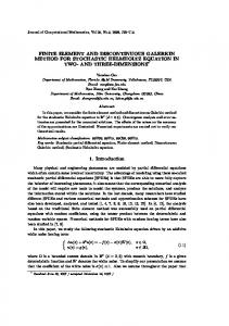
Consider a partition of into two disjoint subdomains 1 and 2 , such that the slip surface slip is entirely contained in 2 . Assume 2 to be contained in the interior of , so that @ is contained in @ 1 (in other words, @ 2 does not intersect @ ), and define ÿ : @ 1 \ @ 2 @ 2 . The partition of the air-gap

is shown in Figure 1.

COMPEL 20,2


452

Figure 1. Partition of air-gap in different sub-regions. The slip surface Uslip contained in O2 is dashed

The possible hanging nodes resulting from the relative movement of the mesh consistent with the rotor with respect to the mesh consistent with the stator are contained in the region 2 . Thus, it is possible to discretise the problem in 2 by using a discontinuous finite element method, which allows for hanging nodes, and a standard continuous method in 1 . However, the two methods have to be coupled at the interface ÿ. Setting ui : uj i , i 1; 2, problem (8) can be written as the following transmission problem: u1 0

in 1 ;

9

u2 0

in 2 ;

10

on @ ;

11

on ÿ;

12

u1 g u1 u2

ru1 n 1 ÿru2 n 2

on ÿ

13

(n i is the outward unit normal to the region i , i 1; 2). The discontinuous method adopted here for the discretisation of problem (9)(13) in 2 is the LDG method (see Cockburn and Shu (1998) and Castillo et al. (n.d.)).

3. The LDG method Before dealing with the complete discretisation of problem (9)-(13), the formulation and main properties of the LDG method for the Laplace equation as presented in Castillo et al. (n.d.) are briefly recalled in this section. Consider the model problem:


ÿu f u uD ru n qN n

in ; on TD ;

14

on TN ;

where is a bounded domain of RRd , d 2; 3, n is the outward unit normal to its boundary @ T D [ T N , and the d ÿ 1-measure of TD is non-zero. Introducing q : ru, problem (14) can be rewritten as the following system of first-order equations: q ru

in ;

ÿr q f u uD

in ;

on TD ;

q n qN n

on TN :

15 16 17 18

The LDG method is obtained by the following three steps: (1) Write a weak formulation of the problem, by multiplying equations (15) and (16) by arbitrary, smooth test functions r and v, respectively, and integrating by parts over each element K of the grid T h with which the domain is triangulated. The subscript h denotes the mesh size, and T h can have hanging nodes and elements of several shapes. (2) Replace the exact solution q; u by its approximation qh ; uh in the finite element space Q h Vh , where: Q h : fq 2 L2 d : q K 2 SKd ; 8K 2 T h g; Vh : fu 2 L2 : u 2 SK; 8K 2 T h g; K

and SK typically consists of polynomials (e.g. SK P k K, the space of the polynomials of degree at most k on K). Notice that the functions in the spaces Q h and Vh are completely discontinuous across interelement boundaries. (3) Approximate the traces of u and q on the boundary of the elements by introducing the so-called numerical fluxes, denoted in the following by bh . b uh and q


453

COMPEL 20,2

Then, the method consists in finding qh ; uh 2 Q h Vh such that: Z Z Z b q h r dx uh r r dx ÿ uh r n K ds 0 K

K

Z


454

@K

Z K

q h rv dx ÿ

19

Z

@K

b h n K ds vq

K

f v dx;

20

for all test functions r; v 2 SKd SK, for all elements K 2 T h ; here and in the following, nK denotes the outward unit normal to @K. Some notation needs to be introduced, before defining the numerical fluxes bh in equations (19) and (20). Let K and K ÿ be two adjacent elements b uh and q of T h , and let x be an arbitrary point of the set e @K \ @K ÿ , which is assumed to have a non-zero d ÿ 1-dimensional measure. Since K and K ÿ can be non-matching, e is not necessarily a complete face of T h . Let n and n ÿ be the corresponding outward unit normals at the point x. For a function q; u smooth inside each element K , denote by q ; u the traces of q; uon e from the interior of K . Then, the mean values ffgg and jumps at x 2 e are defined as follows: ffugg : u uÿ =2

ffqgg : q q ÿ =2;

u : u n uÿ n ÿ

q : q n qÿ n ÿ :

Note that the jump in u is a vector and the jump in q is a scalar which only involves the normal component of q. With this notation, the numerical fluxes in equations (19) and (20) are defined as follows: if e is inside the domain , b uh je : ffuh gg uh ; bh je : ffq h gg ÿ uh ÿ q h ; q and, if e lies on @,

uD on TD ; u h on TN ;

22

q h ÿ uh ÿ uD n on TD ; qN on TN :

23

b uh je : and

bh je : q

21

Here, the scalar and the vector are auxiliary parameters whose purpose is to enhance the stability and accuracy properties of the LDG method, see Cockburn and Shu (1998) and Castillo et al. (n.d.). For > 0 and arbitrary, the LDG method in equations (19) and (20) with numerical fluxes defined by equations (21)-(23) has a unique solution and is consistent. Furthermore, since b uh does not depend on q h , the unknown q h can be computed element by


element in terms of uh , by using equation (19), and then substituted into equation (20), giving rise to a problem in the uh unknown only; see Cockburn and Shu (1998) for more details. This local solvability gives its name to the LDG method. A complete a priori error analysis of the LDG method for elliptic problems has been derived in Castillo et al. (n.d.). Here, the case where the parameters and are constants independent of the mesh size h is considered. For this particular case, the following error estimates can be proved. Theorem 1. Assume and to be independent of the mesh size h, > 0, and the local spaces SK to contain the polynomials of degree k, i.e. P k K SK. Then, if the solution q; u of equations (15)-(18) is sufficiently smooth, we have the a priori error estimates for the LDG solution: 1

jju ÿ uh jjL2 Chk2 ;

jjq ÿ q h jjL2 Chk ;

with a constant C independent of h. It should be remarked that the a priori estimate for u falls half a power of h short from being optimal. However, it has been proved in Castillo et al. (n.d.) that it is possible to select and in such a way that the accuracy of the LDG method increases. For example, on Cartesian grids, p can be chosen so that the orders of convergence for u and q increase by h, or, on general grids, if is chosen mesh-dependent and of order 1=h, the optimal rate k 1 can be obtained for u. Nevertheless, the simplest choice const is justified by the numerical results of Castillo et al. (n.d.) where no decrease in the actual numerical rates of convergence was observed. 4. Coupling LDG/continuous elements In this section, the complete discretisation of the two-dimensional problem (9)(13) is presented. It is clear from section 3 that, despite the advantage of allowing for non-matching elements, the LDG method requires a high number of degrees of freedom. In order to limit the global number of degrees of freedom, problem (9)-(13) is discretised by using the LDG method just in 2 , and a standard continuous finite element method in 1 , as mentioned at the end of section 2. Let T 1h and T 2h be triangulations of 1 and 2 . Assume, to fix the ideas, that 1 T h consists of triangles. By introducing the auxiliary variable q : ru2 in 2 as in section 3, the solution q, u2 and u1 of problem (9)-(13) satisfies: Z Z Z q r dx u2 r r dx ÿ u2 r n K ds 0 24 K

K

Z

@K

2

K

q rv dx ÿ

Z @K

v2 q n K ds 0

25

for piecewise smooth test functions r and v2 , and for all elements K 2 T 2h , and:


455

Z

COMPEL 20,2


456

1

1

1

ru rv dx ÿ

Z ÿ

ru1 n 1 v1 ds 0;

26

for smooth test functions v1 , with v1 j@ 0. Equations (24), (25) and (26) have to be coupled through the transmission conditions (12) and (13). Condition (13) is imposed by replacing ru1 n 1 with ÿq n 2 in equation (26), which becomes: Z Z 1 1 ru rv dx q n 2 v1 ds 0; 27

1

ÿ

while condition (12) will be imposed at the discrete level by choosing the numerical fluxes in the LDG method in a suitable way. The exact solution q; u2 ; u1 in equations (24), (25) and (27) is then approximated by the triple q h ; u2h ; u1h in the finite element space Q h Vh Wh , where: Q h : fq 2 L2 2 2 : q K 2 SK2 ; 8K 2 T 2h g; Vh : fu2 2 L2 2 : u2 K 2 SK; 8K 2 T 2h g; Wh : fu1 2 H 1 1 : u1 K 2 P ` K; 8K 2 T 1h g: Remark that Wh is the standard continuous P ` finite element space. Finally, the traces of u2 and q in equations (24), (25) and (27) are approximated by numerical fluxes b u2h and^ q h . As mentioned above, the numerical fluxes have to take care of imposing the transmission condition (12). The edges that lie on the interface ÿ are considered as ``Dirichlet'' edges from bh are therefore the LDG side, with Dirichlet datum uD u1h , and b u2h and q 2 defined on e @K, K 2 T h , as follows (cf. equations (21)-(23)): 2 ffuh gg u2h if e @K n ÿ; 2 b 28 uh je u1h if e @K \ ÿ: and

bh je q

ffqh gg ÿ u2h ÿ q h q h ÿ u2h ÿ u1h n 2

if e @K n ÿ; if e @K \ ÿ:

29

bh defined in equations (28) and (29), the discrete formulation of With b u2h and q the problem reads as follows: find q h ; u2h ; u1h in Q h Vh Wh , with u1h satisfying an approximation of the inhomogeneous boundary condition (11), such that: Z Z Z 2 b q h r dx uh r r dx ÿ 30 u2h r n K ds 0; K

K

@K

Z

2

K

qh rv dx ÿ

Z @K

b n K ds 0; v2 q

31

for all test functions r; v2 2 Q h Vh and for all elements K 2 T 2h (cf. equations (19) and (20)), and Z Z 1 1 bh n 2 v1 ds 0; ruh rv dx q 32 Downloaded by UNIVERSITA DEGLI STUDI DI PADOVA At 03:44 12 December 2014 (PT)

1

ÿ


457

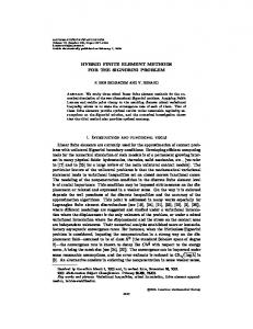
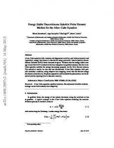
for all test function v1 2 Wh such that v1 j@ 0. A detailed description of all the terms to be implemented for the coupled formulation is reported in the Appendix. 5. Numerical results The test case refers to a 90ë sector of a cylindrical capacitor filled with air, shown in Figure 2. This problem has the analytical solution ue ÿui lnr=ri and the particular case where re 7, ri 5, ui 0 u ui lnr e =ri and ue 1 is considered. The slip surface slip is set at r 6, and splits the domain into upper and lower parts u and ` . The domain is meshed independently in u and ` with straight triangular elements, so that elements on the two sides of slip can be non-matching. The region 2 (LDG elements) consists of all triangles having at least one node on slip .The different meshes are identified by a code of the form Nu ÿ N` which specifies the number of regular subdivisions on the upper and lower side of slip . In all experiments, P 1 polynomials are used everywhere: standard continuous P 1 in 1 , and discontinuous P 1 in 2 . Hereafter, the coupled formulation will be referred to as LDG/P1. As an example, the mesh for the test case 10-30 is shown in Figure 3. Figures 4, 5 and 6 show the behaviour of the solution along the line r 6:1 with different choices of the parameters and , and with different formulations and meshes. The influence of on the solution is reported in Figure 4. Taking the 30-30 case as a reference, one can see that in both the 20-30

Figure 2. Test case: cylindrical capacitor

COMPEL 20,2


458

Figure 3. Formulation LDG/P1: 10-30 mesh

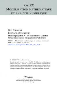
Figure 4. Influence of the choice of b on the solution



459

Figure 5. Influence of the choice of a on the solution

Figure 6. Comparison between P1 and coupled LDG/P1 formulations

COMPEL 20,2


460

Figure 7. Radial behaviour of the solution

and 10-30 meshes, the choice 0; 0 results in solutions which are closer to the correct one than those obtained with 1; 1. Furthermore 1; 1 produces a non-physical slope in the solution. Due to the better behaviour of the solution for 0; 0, the next comparisons are all carried out with this choice of the parameter. The influence of a on the solution is reported in Figure 5. Large values of result in solutions which become further apart from the correct one as increases. Values of which are comparable to the mesh size give rise to similar results. A comparison between the solutions obtained with the coupled LDG/P1 formulation ( 1; 0; 0) and with a purely P1 one is shown in Figure 6. In the case of matching grids the LDG/P1 solution is almost identical to the one obtained with standard P1 elements. As the difference between Nu and N` increases, there is a degradation in the quality of the solution, with an average error of about 5 per cent for the 10-30 case. As shown in Figure 7 (graph along the 89 line) most of the error tends to be confined to the coarse elements of the 2 region. 6. Conclusions The proposed purely FE method, coupling standard continuous and discontinuous elements, allows for dealing with non-matching grids by preserving a sparse structure of the coefficient matrix of the resulting algebraic linear system. The numerical evidence provided shows that only modest inaccuracies are introduced by the method in the case of highly non-matching grids. Currently, further tests on problems of industrial complexity are under way.


References Alotto, P., Bertoni, A. and Molfino, P. (1998), `À combined FEM-BEM and tableau analysis for the modelling of moving devices fed by arbitrary lumped parameters electrical circuits'', in Proceedings of 4th Int. Workshop on Electric and Magnetic Fields from Numerical Models to Industrial Applications, 12-15 May 1998, Marseille, France, pp. 243-8. Castillo, P., Cockburn, B., Perugia, I. and SchoÈtzau, D. (n.d.), `Àn a priori error analysis of the local discontinous Galerkin method for elliptic problems'', SIAM J. Num. Anal., to appear. Cockburn, B. (1999), ``Discontinuous Galerkin methods for convection-dominated problems'', in Barth, T. and Deconink, H. (Eds), High-Order Methods for Computational Physics, Vol. 9 of Lecture Notes in Computational Science and Engineering, Springer Verlag, Berlin, pp. 69-224. Cockburn, B. and Shu, C.W. (1998), ``The local discontinous Galerkin finite element method for convection-diffusion systems'', SIAM J. Num. Anal., Vol. 35, pp. 2440-63. Kurz, S., Fetzer, J. and Kube, T. (1996a), ``BEM-FEM coupling in electromagnetics: a 2-D watch stepping motor driven by a thin wire coil'', in Proceedings of 7th IGTE Symposium on Numerical Field Computation in Electrical Engineering, 23-25 September 1996, Graz, Austria, pp. 492-6. Kurz, S., Fetzer, J. and Lehner, G. (1996b), ``Three-dimensional transient BEM-FEM coupled analysis of electromagnetics levitation problems'', IEEE Trans. Magn., Vol. 32 No. 3, pp. 1062-5. Rapetti, F., Buffa, A., Bouillaut, F. and Maday, Y. (2000), ``Simulation of a coupled magnetomechanical system through the sliding-mesh mortar element'', COMPEL, to appear. Stenberg, R. (1998), ``Mortaring by a method of J.A. Nitsche'', in Idelsohn, S., Onate, E. and Dvorkin, E. (Eds), Computational Mechanics, New Trends and Advances, CIMNE Barcelona, Spain. Taukerman, I.A., Konrad, A. and Lavers, J.D. (1992), `À method for circuit connections in time dependent eddy current problems'', IEEE Trans. Magn., Vol. 28 No. 2, pp. 1299-302.

Appendix The detailed formulation of the coupled LDG/continuous method, obtained by substituting the numerical fluxes (28) and (29) in equations (30), (31) and (32), reads as follows: find q h ; u2h ; u1h in Q h Vh Wh , with u1h satisfying an approximation of the inhomogeneous boundary condition (11), such that, for all test functions r; v2 2 Q h Vh and for all elements K 2 T 2h , Z Z q h r dx u2h r r dx K K X hZ 1 ÿ n K u2h r n K ds 2 e e@Knÿ Z i 1 2;ext ÿ r n K ds n ext K uh 2 e X Z ÿ u1h r n K ds 0 e@K\ÿ

e


461

COMPEL 20,2

Z ÿ

K

X hZ

qh rv2 dx

e@Knÿ

Z

462

v2

e@K\ÿ


e

1 2

ÿ n K qh n K ds

ext ext qext ds h n K ÿ n K qh n K 2 Z Ze i v2 n ext ÿ u2h v2 ds ÿ u2;ext K n K ds h e e Z X hZ 2 v qh n K ds ÿ u2h v2 ds

1

v2

Z

e

e

e

i

u1h v2 ds 0

(the superscript `èxt'' denotes quantities taken from outside K), and for all test function v1 2 Wh such that v1 j@ 0, Z Xh Z ÿ ru1h rv1 dx ÿ qh n 2 v1 ds

1

Z

e

u2h v1 ds ÿ

Z e

eÿ

i

e

u1h v1 ds 0