discontinuous finite element visualization - Semantic Scholar

8th International Symposium on Flow Visualisation (1998)

DISCONTINUOUS FINITE ELEMENT VISUALIZATION A. O. Leone

P. Marzano

E. Gobbetti

R. Scateni

S. Pedinotti

Keywords: visualization, high-order finite elements, discontinuous fields, mesh refinement

Abstract The aim of this work is the study and the implementation of appropriate visualization techniques for high-order discontinuous finite element data in two and three-dimensions. In particular, we are dealing with field discontinuity and deformed cells. Such data are produced for example by chemical simulations, by fluid dynamics simulations, or, in general, anywhere high accuracy on boundary domain description is required. 1 Motivations Finite element methods are well suited to represent physical processes in simulation programs. Several applications in the field of fluid dynamics need to represent discontinuous fields defined on high-order finite elements cells[1]. Such data are produced for example as an output from chemical simulation processes. The combination of discontinuous finite element simulation methods, topologically unstructured grids, and high-order polynomial approximations of fields and geometries allows programs to handle a variety of situations in which standard approaches usually fail[2]. In particular, structured grids suffer from heavy limitations when dealing with complicated geReceived January 1, 1998. Accepted March 10, 1998.

ometry or when trying to adapt to local features of the solution. Furthermore, discontinuous finite element methods ensure time accuracy of the solution to be obtained by using high order polynomial approximations within each element (cell), thus being particularly well suited to unstructured grids. Finally, when high accuracy in the computational domain boundary description is required by a finite element simulation program, it is often necessary to deal with geometrically deformed cells, as the higher-order shape of these cells may give a better approximation of the boundaries than a linear one[3]. Common visualization approaches do not offer the possibility to handle discontinuities and this research area seems to be completely uninvestigated when discontinuities are combined with unstructured topology. The aim of our research is to supply general purpose visualization tools and techniques for representing meshes made up of topologically different cells (a combination of triangles, quadrilaterals, and other generic convex polygons in the bidimensional case; a combination of tetrahedra together with hexahedra, and generic convex polyhedra in the threedimensional case) on which discontinuous scalar and vector fields are defined. Also, high-order polynomial parametric description of the geometry must be represented graphically along with the field values defined over it.

Contact author: A. O. Leone1 , P. Marzano, E. Gobbetti, R. Scateni, S. Pedinotti2 1

CRS4 - Centro di Ricerca, Sviluppo e Studi Superiori in Sardegna, Via N. Sauro 10, 09123 Cagliari, Italy. (http://www.crs4.it/) 2 ENEL - Centro Ricerca Termica, Pisa, Italy

1–1

A. O. Leone, P. Marzano, E. Gobbetti, R. Scateni, S. Pedinotti

2 Research Activity 2.1 High order polynomial approximation Standard visualization tools and techniques are optimized for the case when each variable defined over a cell has a linear behavior. In particular, current graphics hardware only implements linear interpolation of colors (Gouraud shading). In order to obtain interactive performance, one of the main problems that has to be faced is to linearly approximate polynomial functions for rendering purposes. In our approach, such approximation has been performed using the Longest Side Midpoint Insertion mesh refinement algorithm[4]. At each step of the iterative method, a cell to be refined, with respect to a defined error estimation and a given threshold, is split along its longest side in two cell. The same splitting is recursively applied to any cell adjacent to the same side (see fig. 1).

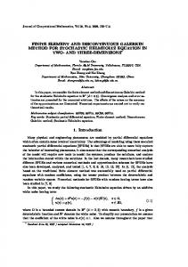
Fig. 2. A quadratic field represented by isolines

2.2 Discontinuity Representation An effective representation of discontinuities is a major problem to be solved for discontinuous fields. Discontinuity is a fundamental information in the simulation process, as discrepancy in function values at cell interfaces provides information on solution convergence.

Fig. 1. The Longest Side Midpoint Insertion algorithm. The top cell starts the recursion

This method has been proven to produce a conforming and good quality mesh[5] and to converge in a finite number of computational step to a linear approximation of the function defined on the original mesh, given a tolerance value, both in 2D and 3D. The use of a grid refinement approach makes it possible to use, on the refined set of cells, standard visualization methods for linear functions. As the visualization algorithms have to deal only with linear functions, it is possible to obtain interactive performance. Figure 2 shows the isolines representation of a field defined over a quadratic triangular element where the refinement alghoritm has been applied. 1–2

Fig. 3. Visualization of discontinuities

To visualize discontinuity we decided to handle each cell as a separate entity by representing function values at a vertex independently on each cell sharing that vertex (see fig. 3). This way to describe the actual solution has then been combined with the representation of the average solution for each vertex obtained by the values of the function in the cells incident on it. The possibility to describe both the actual and

Discontinuous Finite Element Visualization

the average solution showed to be a good way for emphasizing discontinuities. Both solutions are represented by classical visualization techniques (i.e., by isocontours and color mapping), as described in the following section. Another approach for discontinuity representation consists in mapping the variance of the discontinuous solution on the edges of the underlying grid. In this way discontinuities are made evident within the mesh and their visualization can be combined with isocontours or color mapping of either the actual or the average solution. Figure 4 shows one of these possible combinations applied to the same dataset depicted in figure 3.

Fig. 4. Visualization of derived average and variance fields

2.3 Deformed Geometry While visualizing this kind of data, we had the problem to represent deformed cells with computer graphics primitive that are linear. Our solution is to produce a good approximation of such cells with a set of linear cells. We applied the Longest Side Midpoint Insertion algorithm even in this case by considering the physical coordinates of the mapped cell control points as fields defined over the cell. This way, the same finite element interpolation formulas can be used to compute the geometric mapping of the referrer cell into the physical space (see fig. 5). Figure 6 shows how quadratic boundaries of a bidimensional dataset are well represented by

referrer space

physical space

Fig. 5. Deformation of a P2 cell. All sides are given by 3 points coordinates in the physical space

using a small amount of additional linear cells obtained by the refinement process.

Fig. 6. Visualization of quadratic boundaries. Thick lines represent sides of added elements

2.4 Error estimation One of the critical points of the method presented resides in estimating the error introduced by considering an element as if it was linear. Such error drives the refinement of the mesh and it is used to stop the splitting process when the accuracy reaches a value below a given threshold. Because the refinement is performed both for geometric that for field representation, we used two different error measures. For each cell, the geometric error is computed as the maximum distance of the control points in the physical space from the corresponding point of the linearly mapped cell (see fig. 7). 1–3

A. O. Leone, P. Marzano, E. Gobbetti, R. Scateni, S. Pedinotti

Fig. 7. Error estimation: distance C-C’ is the geometric error for the deformed cell

Fig. 8. Error estimation: field error is given by formula (1)

The global geometric error for a mesh is defined by the maximum error computed on each cell. If this is greater than the given threshold, then the cell with the biggest error is splitted according to the refinement alghorithm. The field error, on the other hand, is computed as the maximum absolute difference between the field values on the control points and the corresponding linearly interpolated values. In the case of the second order element showed in figure 8, the error is computed by the formula

topologies within a simple parametric user interface. MIGAVIS has been developed by augmenting the object-oriented Visualization Toolkit by Schroeder, Martin and Lorensen[6] with new classes for handling high-order finite elements and discontinuity information. The application has been completely developed in C++ and the development platform was an IRIX 5.3 Silicon Graphics workstation. A parametric user interface implemented in OSF/Motif allows an easy interaction with data. The system offers the possibility of visualizing:



|F2 −  err = max  |F4 − |F6 −

F1 +F3 | 2 F3 +F5 | 2 F5 +F1 | 2

  

(1)

where Fi is the field value on the i-th control point. Here again, the global field error for a mesh is defined by the maximum error computed on each cell. If this is greater than the given threshold, then the cell with the biggest error is splitted according to the refinement alghorithm. 3 Implementation The first practical result of our research was the implementation of a visualization system for the representation of discontinuous fields defined on high order finite element grids. The system, called MIGAVIS, combines different techniques for representing discontinuities on unstructured 1–4

• the wire-frame grid on which the solution is defined; • the actual discontinuous solution; • the average solution. Both the actual and the average solution can be described by either a scalar representation (through isocontours or color mapping) or a vector representation (through glyphs or hedgehogs). The user can interactively select the scalar field (i.e., a specific solution corresponding to a variable in the simulation process) for scalar visualization and/or the scalar fields for vectorial visualization. The vector visualization is obtained combining different scalar solutions.

Discontinuous Finite Element Visualization

The variance of the solution can be mapped on grid edges whenever desired, thus emphasizing discrepant values at cell interfaces just in correspondence of their location within the grid. All the visualization methods can be combined to produce a single image. The visualization system is integrated with an interface that gives the possibility to interactively modify the parameters of the visualization process:

As an example, we can consider two 2D cases recently studied. The first one is the flow calculation for a first stage steam turbine nozzle. In this case the computation was aimed at evaluating the behaviour of a new profile designed to reduce the blades erosion due to oxide particles. Figures 9 and 10 show the Mach isolines for the old and for the new slanted profile.

• parameters for mesh refinement process; • colormaps for variance and for all solution and grid representations; • value ranges for variance and for all solution representations; • number of contours; • glyphs and hedgehogs parameters (height, scale, etc. ); • parameters for linear and non-linear colormaps;

Fig. 9. 2811 vertex and 5304 cells

• scale factor for Cartesian axes; • offset factor for visualized objects with respect to cartesian axes. 4 Results The MIGAVIS visualization system is currently being used at ENEL Research Department in Pisa (Polo Termico) as a suitable post-processor for MIGALE, a discontinuous finite elements solver for compressible and viscous flows. The main application of MIGALE is the study of turbomachinery flows. The main reason to use MIGAVIS as visualizer for a specific CFD solver is given by the particularity of the discontinuous finite elements method. As a matter of fact, the visualization of solution discontinuities is very useful in order to highlight computational lack either in convergence or in precision. The visualization of discontinuities is especially important in 3D simulation, that represents the most challenging task.

Fig. 10. 3430 vertex and 6486 cells

The second case is an optical probe for density measurements in the wet steam region of turbines. The probe consists of a steel cylinder having a lenghtwise cavity, the laser beam emitted from one side of the cavity is collected by a detector placed on the opposite side. Figures 11 and 12 shows the fully developed computations of different precisions. Mach contours 1–5

A. O. Leone, P. Marzano, E. Gobbetti, R. Scateni, S. Pedinotti

for isoparametric linear elements have evident discontinuities in the wake and near the solid boundary. Quadratic elements coupled with cubic boundaries representation eliminate such discontinuities.

Fig. 13. The same dataset of fig 12 refined up to 7337 cells

Fig. 11. 2534 vertex and 4919 linear elements

Fig. 12. elements

2534 vertex and 4919 quadratic

Figure 13 shows the same dataset refined up to a 50% added cells to obtain a more accurate representation of the field under analysis. References [1] Bassi F, Mariotti G, Pedinotti S, and Rebay S. Recent developments on the solution of the full navier-stokes equations using a discontinuous finite element method. Proc IX Int.l Conf. on Finite Elements in Fluids, New Trends and Applications, Venice, Italy, pp 529–539, Oct 15–21 1995. 1–6

[2] Bassi F, Rebay S, Mariotti G, and Pedinotti S. A high order accurate discontinuous finite element method for inviscid and viscous turbomachinery flows. Proc 2nd European Conference on Turbomachinery - Fluid Dynamics and Thermodynamics, Antwerp, Belgium, Mar 5–7 1997. [3] Kardenstuncer K and Norrie D. Finite Element Handbook. McGraw-Hill, 1995. [4] Rivara M and Inostroza P. A discussion on mixed (longest-side midpoint insertion) delaunay techniques for the triangulation refinement problem. Proc 4th International Meshing Roundtable, Sandia Nat.l Labs, pp 335–346, October 1995. [5] Rivara M and Levin C. A 3-d refinement algorithm suitable for adaptive and multi-grid techniques. Communications in Applied Numerical Method, Vol. 8, pp 281–290, 1992. [6] Schroeder W, Martin K, and Lorensen B. The Visualization Toolkit - An Object-Oriented Approach to 3D Graphics. Prentice-Hall, 1996.