Discovering Interesting Association Rules by. Clustering. Yanchang Zhao, Chengqi Zhang and Shichao Zhang. Faculty of Information Technology, Univ. of ...
Discovering Interesting Association Rules by Clustering Yanchang Zhao, Chengqi Zhang and Shichao Zhang Faculty of Information Technology, Univ. of Technology, Sydney, Australia {yczhao, chengqi, zhangsc}@it.uts.edu.au
Abstract. There are a great many metrics available for measuring the interestingness of rules. In this paper, we design a distinct approach for identifying association rules that maximizes the interestingness in an applied context. More specifically, the interestingness of association rules is defined as the dissimilarity between corresponding clusters. In addition, the interestingness assists in filtering out those rules that may be uninteresting in applications. Experiments show the effectiveness of our algorithm. Keywords: Interestingness, Association Rules, Clustering
1
Introduction
Association rule mining does not discover the true correlation relationship, because high minimum support usually generates commonsense knowledge, while low minimum support generates huge number of rules, the majority of which are uninformative [8]. Therefore, many metrics for interestingness have been devised to help find interesting rules while filtering out uninteresting ones. The interestingness is related to the properties of surprisingness, usefulness and novelty of the rule [5]. In general, the evaluation of the interestingness of discovered rules has both an objective (data-driven) and a subjective (userdriven) aspect [6]. Subjective approaches require that a domain expert work on a huge set of mined rules. Some adopted another approach to find “Optimal rules” according to some objective interestingness measure. There are various interestingness measures, such as φ-coefficient, Mutual Information, J-Measures, Gini indes, Conviction, collective strength, Jaccard, and so on [11]. To the best of our knowledge, for a rule A → B, most existing interestingness measures are computed with P (A), P (B) and P (A, B). In a quite different way, we devise a measure of interestingness by clustering. By clustering the items, the distances or dissimilarities between clusters are computed as the interestingness to filter discovered rules. Experiments show that many uninteresting rules can be filtered out effectively and rules of high interestingness remain. Then a domain expert can select interesting patterns from the remaining small set of rules. The rest of the paper is organized as follows. In Section 2, we introduce the related work in studying the interestingness of association patterns. The idea of using clustering to measure the interestingness is described in detail in Section 3. Section 4 shows our experimental results. Conclusions are made in Section 5.
2
Related Work
The measures of rule interestingness fall into two categories, subjective and objective. Subjective measures focus on finding interesting patterns by matching against a given set of user beliefs. A rule is considered interesting if it conforms to or conflicts with the user’s beliefs [2, 9]. On the contrary, objective ones measure the interestingness in terms of their probabilities. Support and confidence are the most widely used to select interesting rules. With Agrawal and Srikant’s itemset measures [1], those rules which exceed a predetermined minimum threshold for support and confidence are considered to be interesting. In addition to support and confidence, many other measures are introduced in [11], which are φ-coefficient, Goodman-Kruskal’s measure, Odds Ratio, Yule’s Q, Yule’s Y, Kappa, Mutual Information, J-Measure, Gini Index, Support, Confidence, Laplace, Conviction, Interest, Cosine, Piatetsky-Shapiro’s measure, Certainty Factor, Added Value, Collective Strength, Jaccard and Klosgen. Among them, there is no measure that is consistently better than others in all application domains. Each measure has its own selection bias. Three interest measures, any-confidence, all-confidence and bond, are introduced in [10]. Both all-confidence and bond are proved to be of downward closure property. Utility is used in [2] to find top-K objective-directed rules in terms of their probabilities as well as their utilities in supporting the user defined objective. UCI (Unexpected Confidence Interestingness) and II (Isolated Interestingness) are designed in [3] to evaluate the importance of an association rule by considering its unexpectedness in terms of other association rules in its neighborhood.
3 3.1
Measuring Interestingness by Clustering Basic Idea
There are many algorithms for discovering association rules. However, usually a lot of rules are discovered and many of them are either commonsense or useless. It is difficult to select those interesting rules from so many rules. Therefore, many metrics have been devised to help filter rules, such as lift, correlation, utility, entropy, collective strength, and so on [2, 7, 11]. In a scenario of supermarket basket analysis, if two items are frequently bought together, they will make a frequent item set. Nevertheless, most frequent item set are commonsense. For example, people who buy milk at a supermarket usually buy bread at the same time, and vice versa. So “milk→bread” is a frequent pattern, which is an association rule of high support and high confidence. However, this kind of “knowledge” is useless because everyone know it. The itemset composed of hammer and nail is another example. On the contrary, the rule “beer→diaper” is of high interestingness because beer has little relation with diaper in the commonsense and they are much dissimilar with each other.
From the above examples, we can see that the itemsets which are composed of “similar” items are uninteresting. That is to say, the frequent itemsets consisting of “dissimilar” items are interesting. Therefore, the dissimilarity between items can be used to judge the interestingness of association rules. It is difficult to judge the dissimilarity between items manually. Moreover, it is not easy to design a formula to compute the dissimilarity. Fortunately, the clustering technique can help us to do so. Since the function of clustering is grouping similar objects together, it can help us to know the dissimilarity between objects. From this point, we devise a strategy to measure the interestingness by clustering. By taking each item as an object, the items can be clustered into a couple of groups. After clustering, the items in the same cluster are similar to each other, while two items from two different clusters are dissimilar, and the dissimilarity between them can be judged with the dissimilarity between the two clusters. When all rules have been set interestingness, those rules with high interestingness can be output if a threshold is given. An alternative way it to output the top-k rules with high interestingness, and the user can choose the number of interesting rules to output. Based on the above idea, the interestingness of rules is defined in the following. Definition 1 (Interestingness). For an association rule A → B, the interestingness of it is defined as the distance between the two clusters, CA and CB , where CA and CB denote the clusters where A and B are in respectively. Let Interest(A → B) stand for the interestingness of A → B, then the formula for interestingness is as follows. Interest(A → B) = Dist(CA , CB )
(1)
where Dist(CA , CB ) denotes the distance between cluster CA and CB . The above definition is for the simplest rule, where there is only one item in the antecedent. However, many rules may have several items in the left. For this kind of rules, an expanded definition is given in the following. Definition 2 (Interestingness). For an association rule A1 , A2 , ..., An → B, its interestingness is defined as the minimal distances between clusters CAi and CB , where CAi and CB denote the clusters where Ai (1 ≤ i ≤ n) and B are in respectively. n
Interest(A1 , A2 , ..., An → B) = min{Dist(CAi , CB )} i=1
(2)
For those kinds rule who have multiple items in the consequent, it is easy to expand the above definition for them. Our approach tries to measure the interestingness by clustering items, while most other measures by analyzing the transaction set. Hence, our approach complements other measures of interestingness. 3.2
Our Algorithm
Our algorithm for measuring interestingness by clustering is given in detail in Figure 1.
INPUT: a rule set R, an item set I, and an interestingness threshold T or the number of rules (k) OUTPUT: a set of interesting rules Cluster the itemset I with an existing algorithm (e.g. k-means) for clustering; FOR each pair of clusters Ci and Cj Set Dist(Ci , Cj ) to the distance between the centroids of Ci and Cj ; ENDFOR FOR each rule A1 , A2 , ..., An → B in the rule set R Interest(A1 , A2 , ..., An → B) = minn i=1 {Dist(CAi , CB )} ENDFOR Output those rules whose interestingness is greater than the threshold T, or those top-k rules with high interestingness;
Fig. 1. Algorithm for Measuring the Interestingness of Rules by Clustering.
3.3
How to Choose the Algorithm for Clustering
There are many algorithms for clustering. Which one is suitable for a given application? It should be chosen according to the specific scenario and the requirement of users. Generally speaking, the algorithm should be capable to handle hybrid data. The reason is that most data for association analysis are of hybrid data, so the algorithm for clustering is required to be able to cluster data both of numeric attributes and categorical ones. On the other hand, since the dissimilarity between clusters will be used as the interestingness of rules, the dissimilarity or distance should be easy to judge or compute. There are mainly four categories of algorithms for clustering, namely, partitioning, hierarchical, density-based and grid-based approaches. For densitybased and grid-based ones, the clusters are generated by expanding the denselypopulated regions or combining dense neighboring cells, so it is difficult to judge the dissimilarity between clusters. Fortunately, for partitioning and hierarchical algorithms, the clusters are usually compact and it is easy to compute the dissimilarity between clusters. For k-means or k-medoids algorithms, the mean or medoid is used to represent a whole cluster, so the dissimilarity can be easily computed as the distance between the means or medoids. For hierarchical approaches, single linkage, average linkage, complete linkage, and mean linkage are main measures for calculating the distances between clusters, and they can be used as the dissimilarity. Therefore, partitioning and hierarchical algorithms can be readily used in our approach, while density-based or grid-based ones are not. In our approach, k-means is used as the algorithm for clustering. Since the kmeans algorithm is only for numeric attributes, we adapt it for clustering hybrid data in the following way. The mean is used for numeric attributes, while the mode is used for categorical attributes. The distance between two clusters is defined as the weighted sum of all attributes. Actually, many other algorithms for clustering (see [4]) can be used or can be adapted for our approach.
The shortcoming of our approach is that it is only suitable for clusters of spherical shapes, not for clusters of arbitrary shapes. Therefore, the algorithms which discovers clusters of spherical shapes is needed in our approach. For algorithms which discover clusters of arbitrary shapes, an effective way to calculate the dissimilarity between clusters should be devised to be used in our approach.
4
Experimental Results
In our experiment, we will show the effectiveness of our approach to filter rules of low-interestingness. The real data from supermarket is used in our experiment. There are two datasets: an item set and a basket dataset. The item dataset are of 460 items and seven attributes, and we choose the weight, price, category, and brand as the features for clustering. An attribute of average price is derived from weight and price. In addition, the category is split into three new attributes, with each standing for a level in the hierarchy of category. The first two attributes are numeric, while the last two are categorical. K-means is used for clustering, and we adapt it for hybrid data. For numeric attributes, the representative of a cluster is set to the mean, while it is set to the mode for categorical attributes. As to the three new attributes of category, the high-level category is assigned with great weight while the low-level category with small weight. All together 5800 association rules with both high support and high confidence are discovered with APRIORI algorithm from the transaction data. By clustering the itemset with k-means (k is set to 10), the items are partitioned into ten clusters. The dissimilarities between clusters are computed as the interestingness of corresponding rules. The top rule with highest interestingness is “#33 → #283”, while item #33 is “Run Te” shampoo, and item #283 is “Hu Wang” sauce of 1000ml. Since shampoo and sauce are from totaly different categories, the rule is of high interestingness (0.909). In contrast, rule “#254 → #270” is of very low interestingness (0.231). Item #254 and #270 are respectively sausage and vinegar. The rule is uninteresting because both of them are cooking materials. The count of rules remained when measuring the interestingness by clustering is shown in Figure 2. The value of interestingness ranges from 0 to 1.17. If the interestingness threshold is set to 0.5, then 3167 out of 5800 rules remain because of high interestingness. If those with interestingness less than 1.0 are filtered out, then 1763 rules remain. If the threshold is set to 1.14, only 291 rules remain while all others are filtered out. After filtering, rules of low interestingness are removed. The remaining rules of high interestingness, which Fig. 2. Experimental Result are much less than the original rules, can then be judged and selected by domain experts. 6
Count of Interesting Rules (x1000)
5
4
3
2
1
0
0
0.2
0.4
0.6
0.8
Interestingness Threshold
1
1.2
1.4
5
Conclusions
In this paper, we have presented a new way to judge the interestingness of association rules by clustering. With our method, the interestingness of rules are set to be the dissimilarity of the clusters which the antecedent and the consequent are in respectively. Since the items from different clusters are dissimilar, the rules composed of items from different clusters are of high interestingness. Our method can help to filter the rules effectively, which has been shown in our experiments. In our future research, we will try to combine existing measures of interestingness with clustering to make it more effective. In addition, subjective measures will be taken into account when clustering. For density-based and grid-based algorithms, it is not easy to judge the dissimilarity between clusters, and we will try to adapt them for measuring the interestingness of rules.
References 1. R. Agrawal, T. Imielinski and A. Swami: Mining association rules between sets of tiems in large databases. In Proc. of the ACM SIGMOD Int. Conf. on Management of Data (SIGMOD’93), Washington, D.C., USA, May 1993, pp. 207-216. 2. R. Chan, Q. Yang, and Y.-D. Shen: Mining high utility itemsets. In Proc. of the 2003 IEEE International Conference on Data Mining, Florida, USA, November 2003. 3. G. Dong and J. Li: Interestingness of discovered association rules in terms of neighborhood-based unexpectedness. In Proc. of the 2nd Pacific-Asia Conf. on Knowledge Discovery and Data Mining, Melbourne, Australia, April 1998, pp. 72-86. 4. Erica Kolatch: Clustering Algorithms for Spatial Databases: A Survey. Dept. of Computer Science, University of Maryland, College Park, 2001. http://citeseer.nj.nec.com/436843.html 5. U.M. Fayyad, G. Piatetsky-Shapiro and P. Smyth: From data mining to knowledge discovery: an overview. In Advances in Knowledge Discovery & Data Mining, pp. 1-34, AAAI/MIT, 1996. 6. Alex A. Freitas: On objective measures of rule surprisingness. In Proc. of 2nd European Symp PKDD’98, Nantes, France, 1998, pp. 1-9. 7. Robert J. Hilderman and Howard J. Hamilton: Knowledge discovery and interestingness measures: a survey. Tech. Report 99-4, Department of Computer Science, University of Regina, October 1999. 8. Won-Young Kim, Young-Koo Lee, and Jiawei Han: CCMine: efficient mining of confidence-closed correlated patterns. In Proc. of 2004 Pacific-Asia Conf. on Knowledge Discovery and Data Mining, Sydney, Australia, May 2004, pp.569-579. 9. B. Liu, W. Hsu, S. Chen, and Y. MA: Analyzing the subjective interestingness of association rules. IEEE Intelligent Systems, 15(5):47-55, 2000. 10. E. Omiecinski: Alternative interest measures for mining associations. IEEE Trans. Knowledge and Data Engineering, 15:57-69, 2003. 11. Pang-Ning Tan, Vipin Kumar, Jaideep Srivastava: Selecting the right interestingness measure for association patterns. In Proc. of the Eighth ACM SIGKDD International Conference on Knowledge Discovery and Data Mining, Edmonton, Alberta, 2002, pp. 32-41.