Singapore Management University
Institutional Knowledge at Singapore Management University Research Collection School of Information Systems
School of Information Systems
10-2010
Mining Interesting Link Formation Rules in Social Networks Cane Wing-Ki Leung Ee Peng LIM Singapore Management University,
[email protected]
David LO Singapore Management University,
[email protected]
Jianshu WENG Singapore Management University
Citation Leung, Cane Wing-Ki; LIM, Ee Peng; LO, David; and WENG, Jianshu, "Mining Interesting Link Formation Rules in Social Networks" (2010). Research Collection School of Information Systems. Paper 624. http://ink.library.smu.edu.sg/sis_research/624
This Conference Paper is brought to you for free and open access by the School of Information Systems at Institutional Knowledge at Singapore Management University. It has been accepted for inclusion in Research Collection School of Information Systems by an authorized administrator of Institutional Knowledge at Singapore Management University. For more information, please email
[email protected].
Mining Interesting Link Formation Rules in Social Networks Cane Wing-ki Leung, Ee-Peng Lim, David Lo and Jianshu Weng School of Information Systems Singapore Management University 80 Stamford Road, Singapore
[email protected], {eplim,davidlo,jsweng}@smu.edu.sg ABSTRACT Link structures are important patterns one looks out for when modeling and analyzing social networks. In this paper, we propose the task of mining interesting Link Formation rules (LF-rules) containing link structures known as Link Formation patterns (LF-patterns). LF-patterns capture various dyadic and/or triadic structures among groups of nodes, while LF-rules capture the formation of a new link from a focal node to another node as a postcondition of existing connections between the two nodes. We devise a novel LF-rule mining algorithm, known as LFR-Miner, based on frequent subgraph mining for our task. In addition to using a support-confidence framework for measuring the frequency and significance of LF-rules, we introduce the notion of expected support to account for the extent to which LFrules exist in a social network by chance. Specifically, only LF-rules with higher-than-expected support are considered interesting. We conduct empirical studies on two real-world social networks, namely Epinions and myGamma. We report interesting LF-rules mined from the two networks, and compare our findings with earlier findings in social network analysis.
Categories and Subject Descriptors H.2.8 [Database Management]: Database Applications— Data Mining; J.4 [Computer Applications]: Social and Behavioral Sciences—Sociology
General Terms Experimentation, Algorithms
Keywords Social network analysis, Local structures, Frequent subgraph mining
1.
INTRODUCTION
Link structures in networks are an important piece of information that can help characterizing various types of Permission to make digital or hard copies of all or part of this work for personal or classroom use is granted without fee provided that copies are not made or distributed for profit or commercial advantage and that copies bear this notice and the full citation on the first page. To copy otherwise, to republish, to post on servers or to redistribute to lists, requires prior specific permission and/or a fee. CIKM’10, October 25–29, 2010, Toronto, Ontario, Canada. Copyright 2010 ACM 978-1-4503-0099-5/10/10 ...$10.00.
network, understanding node (user) activities, identifying communities, detecting anomalies, and so on. In particular, dyadic and triadic structures, also known as local structures, have long been utilized for understanding and predicting the dynamics of large and complex networks [16, 11, 3, 15, 14, 13]. In the area of trust prediction in social networks, for instance, the study in [12] analyzes the formation of trust links as a reciprocity effect. Several other studies examine trust propagation based on transitivity, assuming that trust values attached to links in a network would propagate along directed paths to various degrees (e.g. [4, 10]). Previous social network research on local structures however suffers from two common pitfalls. Firstly, they consider only the topological aspect of local structures and ignore the formation order of links in the network. Most research focuses on analyzing the statistical properties and distributions of non-temporal structures in a network [16, 11, 3, 14]. Only recently, researchers have started to address the temporal order of links in specific triadic structures. For instances, Romero and Kleinberg [13] analyze links that might have been formed as a result of directed closure in Twitter, while Leskovec et al. [7] study link sign prediction between a node pair in a triad given different preexisting connections among the triad. Secondly, due to the enormous overheads of enumerating local structures, researchers usually shy away from identifying new interesting local structures that may exist in the networks to be studied and confine their work to simple structures such as dyads and triads, assuming that they are the only interesting ones. Mining local structures beyond simple dyads and triads while considering time ordering of links is very important for understanding how new links and local structures emerge in different networks. In this study, we therefore propose to mine local structures for link formation from directed, temporal social networks. We formalize the notion of Link Formation rule (LF-rule) to capture the formation of a new link from a focal node, called the start node, to another node, called the end node, as a postcondition of existing connections between the two nodes. A LF-rule thus imposes a temporal constraint on the (partial) formation order of the links it contains. Specifically, the new link formed as a postcondition should be introduced to the social network at a later time point than all other links in the same rule. A LF-rule also follows certain structural constraints, defined as Link Formation patterns (LF-patterns). We aim to capture LF-patterns containing multiple dyadic and/or triadic structures among groups of nodes, instead of simple dyads and triads in this work.
Input graph
Mine LF -rules
... Randomize graph
Compute expected support of LF -rules Identify interesting LF-rules Rule evaluation
Figure 1: Methodology overview. Fig. 1 summarizes our multi-step approach to mining interesting LF-rules. We first devise a new LF-rule mining algorithm based on frequent subgraph mining [5, 6, 17], and apply it on a given social network to obtain a set of LF-rules. To account for the extent to which LF-rules exist in the given network by chance, we conduct graph randomization on the original network so as to determine the expected support of LF-rules. Finally, interesting LF-rules with higherthan-expected support are further evaluated manually. We summarize our contributions as follows: • We introduce LF-rule as a general form of link formation rule that considers both the time and label of network links. It allows local structures other than simple dyads and triads to be studied in social networks. • We develop our LF-rule mining algorithm, known as LFR-Miner, by extending gSpan [17, 18]. LFR-Miner generates the complete set of LF-rules that satisfy userspecified constraints on support, confidence, and the maximum number of nodes in each rule (optional). • We apply graph randomization for estimating the expected support of LF-rules. The concept of expected support helps us determine interesting LF-rules for network analysis and network related prediction tasks. • We apply LFR-Miner to two real-world social networks and evaluate the interesting LF-rules with higher-thanexpected support. We also compare and contrast the interestingness of LF-rules in the two networks. Our work is distinct from related studies in several aspects. To the best of our knowledge, this is the first time a comprehensive approach is introduced to conduct link formation analysis in directed, temporal (time-stamped ) social networks with multiple edge labels. The Graph Evolution Rule Miner (GERM) proposed in [1] also mines frequent graph rules (with arbitrary structures) from a single, temporal graph, but does not consider link directions and labels. We are also not aware of any related work that considers expected support of local structures. Secondly, we take a subgraph mining approach to grow and discover complex patterns that satisfy the desired structural constraints, rather than predefining specific patterns to analyze (e.g. in [7, 13]). Lastly, we evaluate the interestingness of LF-rules with respect to the entire network by means of their support, expected support and confidence. Our study serves as a macro-level analysis of local structures, and complements micro-level analysis on pattern occurrences (e.g. [7]). The remainder of this paper is organized as follows. Sect. 2 formally describes our problem definition. Sect. 3 briefly introduces the mining principles of gSpan, and details the design and implementation of our LFR-Miner algorithm. Sect. 4 describes the computation of expected support. Sect. 5 presents our empirical study on real-world datasets. Sect. 6 describes related work, and finally in Sect. 7, we conclude and outline possible extensions of this work.
Notation G u, v, w ρ(u, v) t(u, v) p, q p.s p.e x ˜
2.
Table 1: Basic notations Description The input graph G = (V, E, L, l, T, t). Individual nodes in G. Geodesic distance between u and v in G. Timestamp of the edge from u to v in G. Link Formation patterns (LF-patterns). The start node of the LF-pattern p. The end node of the LF-pattern p. An occurrence of a certain object x in G.
PROBLEM DEFINITION
In this section, we describe relevant preliminary concepts and introduce Link Formation patterns (LF-patterns) as well as Link Formation rules (LF-rules). We then formally define the LF-rule mining problem.
2.1
Preliminaries
We represent a social network as a directed, labeled and time-stamped graph, written as G = (V, E, L, l, T, t). V is a set of vertices/nodes representing individuals in the network. E is a set of directed links/edges representing relationships between individuals. An element (u, v) ∈ E, where u, v ∈ V , is an edge from u to v. L is a finite set of node and edge labels. l : V ∪ E → L assigns labels to elements in V and E. t : E → T is a mapping between edges and their timestamps. Without loss of generality, we represent timestamps as T = {ti |i ≥ 0}, such that ∀ti , tj ∈ T, ti < tj iff i < j. A graph may evolve with new nodes and edges joining at different time points. G can be viewed as a snapshot of the network taken at a certain time point tn , such that G contains nodes and edges that were formed at or before tn . We assume that edges once formed are not removed. Table 1 summarizes other notations used in our discussions. For a given graph G, the geodesic distance from u to v, denoted by ρ(u, v), is the number of edges in the shortest path from u to v. ρ(u, v) and ρ(v, u) may not be equal since G is directed. ρ(u, v) = +∞ if there is no path from u to v.
2.2
Link Formation Patterns and Rules
We study link formation from a focal node s, called the start node, to another node e, called the end node, as a postcondition of existing connections between s and e. Given a link (s, e), we assume that s is the creator or sender of the link, as this is often the case in directed social networks such as Epinions’ web of trust. Further, we are only interested in patterns that are connected or weakly connected, i.e., there exists a path between any two nodes in the pattern, omitting link directions. This is reasonable since we seek to find the structures connecting s and e that may lead to the formation of a new link from s to e. We use the patterns in Fig. 2 and the graph in Fig. 3 as the input graph G as examples throughout this section. For simplicity, all edges in our sample patterns and G carry the same label of “1”, which is omitted in their graphical representation. Nodes marked with s and e in our patterns correspond to the start and the end nodes respectively, while those unlabeled are intermediaries. Link Formation Pattern. A LF-pattern encodes structural constraints on the nodes it contains. This work focuses on patterns containing dyadic and triadic structures among groups of nodes as noted. Furthermore, a LF-pattern im-
s s
e
s
s
e
e
s
e
e p1
p2
p3
p4
p5
Figure 2: Examples of LF-patterns. s and e denote the start node and the end node respectively. t2
C
t6
A
t1 t3
t0
B
E
t7 t4
Example 1. In graph terms, there exists a subgraph isomorphism from p1 to p3 . In such an isomorphism, however, either node s or e in p1 will be mapped to the intermediary in p3 , violating Condition 3 above. Similarly, p2 and p3 are isomorphic in graph terms if we ignore the special nodes s and e, but are considered different LF-patterns. The rationale behind this becomes obvious if we take away the (s,e) link from the two patterns: they encode different connectivity between s and e before the (s,e) link is formed.
t5
D
Figure 3: The sample input graph G. For simplicity, all edges in this graph have the same label, which is omitted in the graph. ti denotes timestamp of edge creation. ti < tj iff i < j. plicitly encodes the temporal constraint that the link (s, e) is formed after all other links in the same pattern. Formally, a LF-pattern is defined as follows: Definition 1 (Link Formation Pattern). A Link Formation pattern, or LF-pattern, is a 4-tuple: p = (Vp , Ep , L, lp ), where Vp is a set of vertices, Ep is a set of edges, L is a finite set of labels, and lp : Vp ∪ Ep → L assigns labels to elements in Vp and Ep . Vp contains (i) a special subset Sp = {s, e}, where s and e are respectively called the start node and the end node of p; (ii) a set of intermediaries Ip between s and e. Ip = Vp \Sp , and it may be an empty set (Ip = ∅). In the edge set Ep , each element (u, v) is a directed edge from u to v, u 6= v, and (s, e) ∈ Ep . Ep captures the connectivity among nodes in Vp , such that either of the following conditions is true: 1. If Ip = ∅, then ∀u, v ∈ Sp , ρ(u, v) = ρ(v, u) = 1. 2. If Ip 6= ∅, then ∀u ∈ Sp , v ∈ Ip , min(ρ(u, v), ρ(v, u)) = 1. Condition 1 means that if Vp contains only s and e, the two nodes must be connected to each other to form a LF-pattern. Condition 2 requires every intermediary to be connected to both s and e, in any direction. Other than Conditions 1 and 2, we allow additional edges to be included in the pattern. Referring to Fig. 2, p1 satisfies Condition 1, and p2 to p5 satisfy Condition 2. Every LF-pattern is at least weakly connected by definition. Definition 2 (Isomorphism of LF-patterns). An isomorphism from a LF-pattern p to another LF-pattern q is a bijective function f : Vp → Vq , such that the following conditions are met:
Based on the assumption that an edge is formed by its sender, we propose the notions of ego-based occurrence and frequency of a given LF-pattern in a graph G: Definition 3 (Ego-based Occurrence). Given a focal node w, known as the ego, in a graph G, an ego-based occurrence, or simply occurrence, of a pattern p is a subgraph p˜ in G that is isomorphic1 to p, such that p˜.s = w, and the timestamp of the edge (˜ p.s, p˜.e), denoted by t(˜ p.s, p˜.e), satisfies the following temporal constraint: t(˜ p.s, p˜.e) >
max
(u,v)∈Ep ˜ p.e) ˜ ˜\(p.s,
t(u, v)
We write the set of ego-based occurrences of p having w as its start node as Γpw . If |Γpw | > 0, we say that p occurred w.r.t. w, and that w supports p. Example 2. Consider p1 and its occurrences in G. It is obvious that p1 did not occur w.r.t. egos B and D. p1 occurred w.r.t. ego A, with p˜1 .s = A and p˜1 .e = E. p1 also occurred w.r.t. ego C, with p˜1 .s = C and p˜1 .e = A. We cannot find an occurrence of p1 w.r.t. ego E: if we take A as node e, then we have t(E, A) < t(A, E), which violates the temporal constraint above. p1 therefore occurred w.r.t. egos A and C only. After determining Γpw for all nodes w ∈ V in G, we can compute the ego-based frequency of p as follows: Definition 4 (Ego-based Frequency). Given p, and the set of Γpw for all nodes w ∈ V in G, let: ½ 1 if |Γpw | > 0, δ(p, w) = 0 otherwise. The ego-based frequency, or simply frequency, of p in G is given by: X freq(p, G) = δ(p, w) w∈V
Example 3. Referring to Example 2, freq(p1 , G) = 2. 1. ∀u ∈ Vp , lp (u) = lq (f (u)). 2. ∀(u, v) ∈ Ep , (f (u), f (v)) ∈ Eq , and lp (u, v) = lq (f (u), f (v)). In other words, freq(p, G) is the number of distinct nodes that acted as the start node of p at least once in G. This ego3. f (p.s) = q.s and f (p.e) = q.e. based frequency measure is anti-monotone, such that given
A subgraph isomorphism from p to q is an isomorphism from p to a subgraph in q. p is a sub-pattern of q only if there exists a subgraph isomorphism from p to q, denoted by p ⊆LF q. q is called a super-pattern of p. Condition 3 above is specific to LF-patterns. Under this condition, p and q are treated as different LF-patterns if the special nodes s and e in the (subgraph) isomorphism from p to q have been changed.
p and q, if p ⊆LF q, then the frequency of p will always be equal to or higher than that of q. Property 1. Given two LF-patterns p and q, if p ⊆LF q, then freq(p, G) ≥ freq(q, G). 1
The term “isomorphic” here shall not be confused with Definition 2: here, the subgraph p˜ that is isomorphic to p is an actual occurrence of p in G, whereas Definition 2 is about isomorphism of LF-patterns.
Proof. We first point out that if q˜ occurred w.r.t. an ego w, then q˜ contains at least one occurrence of p w.r.t. w since p ⊆LF q. Given p˜ occurred w.r.t. w, however, does not necessarily imply that an occurrence q˜ that contains p˜ also occurred w.r.t. w. Now, let’s consider p1 and p2 , where p1 ⊆LF p2 , and p1 occurred w.r.t. egos A and C as discussed. We try to extend occurrences of p1 to obtain those of p2 . p1 ’s occurrence w.r.t. ego A can be extended to an occurrence p˜2 by taking D as the intermediary in p2 . In this case, we can ensure that δ(p2 , A) = 1 = δ(p1 , A) based on Definition 4. p1 ’s occurrence w.r.t. ego C, however, cannot be extended to obtain an occurrence of p2 : if we take B as the intermediary, then t(C, A) < t(C, B), which violates Definition 3. In this case, we have δ(p2 , C) = 0 < δ(p1 , C). We now conclude our proof. Given that p ⊆LF q, for p, p˜ ∈ Γpw , such that p˜ can every ego w with |Γpw | > 0, if ∃˜ q be extended to q˜, then |Γw | > 0 and δ(q, w) = δ(p, w) = 1. Otherwise, |Γqw | = 0, thus δ(q, w) = 0 and δ(q, w) < δ(p, w). Since δ(p, w) ≥ δ(q, w), after summing up δ(q, w) for all egos, we have freq(p, G) ≥ freq(q, G) if p ⊆LF q. Link Formation Rule. We can view the link (s, e) in a LFpattern p as the postcondition of the connections between s and e captured in Ep \{(s, e)}, which we call the precondition of p. We formalize such pre- and post-conditions of link formation as a Link Formation rule (LF-rule). Definition 5 (Link Formation Rule). The Link Formation rule (LF-rule) of a LF-pattern p is defined as r(p) = pa → p. pa is called the precondition of r(p), with the vertex set Vpa = Vp , and edge set Epa = Ep \{(s, e)}. The edge (s, e) ∈ Ep is called the postcondition of r(p). We adopt the support-confidence framework to quantify the frequency and significance of a LF-rule r(p) in G. The support of r(p) is the proportion of nodes in G w.r.t. which p occurred. The confidence of r(p) is the likelihood that (s, e) exists given that pa exists. It takes into account the frequency of pa in G. Note that pa is not a valid LF-pattern due to the missing (s, e) link. Yet, we can still obtain its egobased occurrences and frequency by viewing missing links in G as links that may emerge in the future. Conceptually, we may let the timestamp of a missing (s, e) link be +∞, so that an occurrence of pa will satisfy Definition 3. We now define the support and confidence of a LF-rule. We overload the notation freq(pa , G) to denote the frequency of pa . Definition 6 (Support of LF-Rule). The support of a LF-rule r(p) in a graph G is defined as: supp(r(p)) =
freq(p, G) |V |
Definition 7 (Confidence of LF-Rule). The confidence of a LF-rule r(p) in a graph G is defined as: conf(r(p)) =
freq(p, G) freq(pa , G)
Example 4. Table 2 shows the LF-rule generated from p2 , and reports its support and confidence in G. G has 5 nodes, therefore |V | = 5. p2 occurred w.r.t. ego A only, therefore supp(r(p2 )) = 1/5. pa2 occurred w.r.t. egos A, C, E. Therefore, freq(pa2 , G) = 3, and conf(r(p2 )) = 1/3.
Table 2: LF-rule of p2 . r(p2 ) = pa2 → p2 supp(r(p2 )) s
e
s
e
1/5
conf(r(p2 )) 1/3
Problem Definition. Given a directed, labeled, timestamped graph representing a social network, a support threshold, and a confidence threshold, mine LF-rules that satisfy the given support and confidence thresholds. For trade-off between computational effort and the expressiveness of the mined rules, users could impose a limit on the size of the mined rules, in terms of maximum of nodes in each rule.
3.
MINING LINK FORMATION RULES
We develop our LF-rule mining algorithm, or LFR-Miner, by extending gSpan, a state-of-the-art subgraph mining algorithm based on Depth-First Search (DFS)[17, 18]. Our extensions address two major issues. Firstly, gSpan operates on a database of undirected graphs, but we work with a single directed graph. We thus extend the mining principles in gSpan to consider edge directions in LFR-Miner. Furthermore, the notion of ego we introduced to LFR-Miner essentially serves the purpose of a graph transaction in gSpan’s setting. While gSpan enumerates a pattern’s occurrences in graph transactions to obtain its frequency, we enumerate the occurrences of it w.r.t. egos (nodes). Secondly, gSpan mines for all frequent patterns in the given graph database, while we are interested in LF-patterns, and intermediate patterns that can be grown into LF-patterns. We therefore exploit the structural constraints of LF-patterns and the properties of gSpan’s pattern growth strategy to prune patterns that cannot be grown into LF-patterns. Another issue we have to address is the representation of LF-patterns. Our representation should allow easy enumeration of ego-based occurrence, which imposes a temporal constraint on the (s, e) link. It should also allow us to distinguish between different LF-patterns that are topologically identical in graph terms. We now give a brief overview of gSpan, and refer interested readers to [18, 17] for detailed descriptions. We then discuss the above issues and present our LFR-Miner algorithm.
3.1
Overview of gSpan
Pattern Representation by DFS Code. Given a pattern p, gSpan applies DFS subscripting to all nodes in p to encode the order in which they are traversed in a certain DFS tree. For two “DFS subscripted” nodes vi and vj , i < j iff vi is traversed before vj . Given a DFS tree, the first and the last nodes traversed are called the root and the rightmost vertex respectively. A DFS traversal aims to traverse all nodes in p, and doing so may not require visiting all edges in p. An edge that is visited is called a forward edge, while one that is not visited a backward edge. The path from the root to the rightmost vertex, built upon forward edges, is called the rightmost path. Every DFS tree of p can be mapped to a DFS code, which comprises a DFS edge sequence. Each DFS edge corresponds to one edge in p. gSpan was designed to handle undirected graphs, but as mentioned in [19], a DFS edge with direction can be modeled as a 6-tuple: hi, j, li , l(i,j) , lj , d(i,j) i. i and j are DFS subscripts. The tuple represents a forward edge if i < j, and a backward edge otherwise. li and lj are the
Table 3: DFS codes of p2 and p3 with s as v0 , e as v1 . An asterisk (∗) denotes an empty label. Edge p2 (a) p3 (a) p3 (b) 1 h0, 1, ∗, 1, ∗, →i h0, 1, ∗, 1, ∗, →i h0, 1, ∗, 1, ∗, →i 2 h1, 0, ∗, 1, ∗, →i h1, 2, ∗, 1, ∗, ←i h1, 2, ∗, 1, ∗, ←i 3 h1, 2, ∗, 1, ∗, →i h2, 0, ∗, 1, ∗, →i h2, 0, ∗, 1, ∗, ←i 4 h2, 0, ∗, 1, ∗, ←i h2, 0, ∗, 1, ∗, ←i h2, 0, ∗, 1, ∗, →i node labels of vi and vj respectively, l(i,j) is the edge label, and d(i,j) captures edge direction. We write d(i,j) = → if the edge points from vi to vj ; and d(i,j) = ← otherwise. gSpan defines a linear DFS lexicographic order among all DFS codes, determined based on the lexicographic order among DFS edges (details in [18, 17]). We extend such an order to include edge directions. We define ≺D to be the lexicographic order among d(i,j) ’s, and d(i,j) = → is lexicographically smaller than d(i,j) = ←. ≺D is essential in extending gSpan to directed graphs: when two DFS edges have the same values of i, j, li , l(i,j) , lj but different directions, ≺D is used to determine their lexicographic order. Minimum DFS Code & Rightmost Extension. A pattern p can be represented by multiple DFS codes when there exist multiple DFS trees of it. gSpan defines the canonical label of p as its minimum DFS code, as determined by the DFS lexicographic order. Two patterns p and p0 are isomorphic iff they have the same minimum DFS code. As proven in [18], minimum DFS codes can only be grown from another minimum DFS code by rightmost extension. The essence of this is that non-minimum DFS codes can be pruned while guaranteeing the completeness of mining results. gSpan starts mining with a frequent 1-edge pattern g (in DFS code representation). It then iteratively grows g into larger patterns in the DFS lexicographic order, by performing rightmost extension on it and its children that are minimum DFS codes. A child pattern c of g is formed by adding one edge to g. Rightmost extension states that for c to be a valid DFS code, a backward edge can only grow from the rightmost vertex of g, while a forward edge can grow from vertices along the rightmost path [18].
3.2
DFS Code Representation in LFR-Miner
Our DFS code representation of a LF-pattern always takes s as v0 and e as v1 , thus “forcing” the (s, e) edge to be the first DFS edge. For example, p2 has one DFS code, denoted by p2 (a) in Table 3. p3 has two possible DFS codes, denoted by p3 (a) and p3 (b) in the table, and p3 (a) is smaller than p3 (b) due to ≺D . Note that our representation does not affect the correctness of minimum DFS code computation as all possible DFS codes are built in the same way. The importance of our DFS code representation is threefold. Firstly, it allows us to differentiate LF-patterns that are topologically identical, such as p2 and p3 . Using gSpan’s original representation, p3 (a) and p3 (b) will be pruned as their minimum form is p2 (a). Secondly, it naturally captures the notion of ego in our work. Since v0 corresponds to node s, every match for v0 in the actual graph is essentially an ego that supports the LF-pattern represented by the code. Lastly, by capturing the (s, e) link in the first DFS edge, we can obtain the timestamp t(˜ p.s, p˜.e) once we start to enumerate an occurrence p˜. As we add more edges to p˜, we only need to consider those with timestamps smaller
v0
v1
v2
(a)
v0
v1
v0
v1
v3
v2
v3
v2
(b)
(c)
Figure 4: Patterns that cannot be grown into LFpatterns. Shaded nodes are disallowed to further connect to v0 and/or v1 by rightmost extension. than t(˜ p.s, p˜.e). Our representation therefore facilitates the process of enumerating LF-pattern occurrences. To represent a precondition pa , we still take s as v0 to construct the minimum DFS code of pa , but no longer fix e as v1 since pa has no (s, e) link. Furthermore, we can ignore the temporal order among edges in pa when finding its occurrences in our implementation.
3.3
Rightmost Extension with Pruning
We would like to consider only LF-patterns, and intermediate patterns that can be grown into LF-patterns in LFRMiner. A naive approach to achieve this is to directly adopt gSpan’s rightmost extension to obtain all frequent patterns as intermediate results, and then extract LF-patterns from them in a post-processing step. This approach is, however, undesirable as we would need to process invalid patterns that can never be grown into LF-patterns. Recall that Condition 2 in Definition 1 requires every intermediary to connect with both s (v0 ) and e (v1 ). By exploiting this constraint and the properties of rightmost extension, we identify the following three cases where growing a DFS code c by a DFS edge z will produce a code (pattern) in which an intermediary is disallowed to connect with v0 and/or v1 . We can therefore prune such a code (i.e. we do not need to grow c by z). Case 1: If z = (v0 , vn ) and n > 1, then adding z to c will always exclude v1 from the rightmost path. As a result, vn will be disallowed to connect to v1 by rightmost extension. We therefore do not need to grow c by z. Fig. 4(a) illustrates this case, in which v2 is disallowed to link to v1 . Case 2: If z = (vm , vn ) and 1 ≤ m < n, then we check if all nodes in {vk |1 < k < n}, if any, are connected with both v0 and v1 in c. If not, we do not need to grow c by z. This is because after adding z to c to form a new DFS code c0 , vn will become the rightmost vertex of c0 . Rightmost extension will disallow any node in {vk |1 < k < n} to link to v0 or v1 in any child of c0 . In Fig. 4(b), for example, v2 is disallowed to link to v0 since v3 is the rightmost vertex. Case 3: If z = (vn , vm ) and 2 ≤ m < n (z is a backward edge), we check if vn is connected with both v0 and v1 in c. If not, we do not need to grow c by z to form c0 . The reason is that the two backward edges (vn , v0 ) and (vn , v1 ) are lexicographically smaller than z. They will therefore be disallowed to exist in any child of c0 , so that vn will not be able to link back to v0 and v1 . Fig. 4(c) illustrates this case. In summary, LFR-Miner adopts the principles of rightmost extension for pattern growth, but prunes invalid patterns by addressing the above cases. We evaluate the amount of computational effort saved by the pruning, and more importantly, the completeness of our results in Sect. 5.4.
3.4
The LFR-Miner Algorithm
We now describe the implementation of our LF-rule mining algorithm, LFR-Miner. In what follows, the term “pattern” or “rule” means one in our DFS code representation.
LFR-Miner takes as input a graph G, a support threshold (minS), a confidence threshold (minC), and an optional parameter that specifies the maximum number of nodes in a pattern (maxV ). Algorithm 1 gives the overall flow of LFR-Miner. Similar to gSpan, it starts mining with 1-edge patterns, each of which corresponds to a (s, e) edge (line 3). It then invokes the MineRules procedure in Algorithm 2 to mine for larger patterns in DFS lexicographic order (lines 5-7). Given a pattern p, MineRules invokes the enumeration engine in Algorithm 3 to enumerate the occurrences of p to find the supporting egos of its valid children. Each frequent pattern is recursively grown in MineRules until all its possible valid children have been discovered. Further, LF-rules are generated from frequent LF-patterns. Those that satisfy the minC constraint are produced as output. We now detail Algorithms 2 and 3. Algorithm 1 LFR-Miner(G, minS, minC, maxV ) Input: Output: 1: 2: 3: 4: 5: 6: 7: 8:
Graph G, minimum support minS, minimum confidence minC, maximum no. of nodes in a pattern maxV . LF-rules R.
minSCnt = minS × |V |; R ← ∅; S1 ← all frequent 1-edge patterns in G; sort S1 in lexicographic order; for each p in S1 do p.W ← supporting egos of p in G; MineRules(p, minSCnt, minC, maxV, R); return R;
Algorithm 2 MineRules(p, minSCnt, minC, maxV, R) Input: Output: 9: 10: 11: 12: 13: 14: 15: 16:
p, minSCnt, minC, maxV , LF-rules R. LF-rules mined from p.
Q = GrowAndEnumerate(p, minSCnt, maxV ); for each q ∈ Q do if |q.W | ≥ minSCnt then if q is a LF-pattern then generate r(q); if conf(r(q)) ≥ minC then add r(q) to R; MineRules(q, minSCnt, minC, maxV, R);
MineRules starts by passing the input pattern p to the GrowAndEnumerate procedure to obtain a set of child patterns Q. Each returned child q ∈ Q is associated with its set of supporting egos (q.W ). A frequent q is further processed as follows. If q is a LF-pattern, MineRules generates its LF-rule r(q) by constructing the minimum DFS code of q a , counting freq(q a , G), and then computing conf(r(q)). It is obvious that the supporting egos of q also support q a , thus we only need to try enumerating occurrences of q a w.r.t. nodes that do not support q and calculate freq(q a , G). If r(p) satisfies the confidence threshold, then it is included in the output R (lines 12-15). At line 16, each frequent q is recursively grown by MineRules, until all of its children have been processed. Infrequent patterns are not further processed because their super-patterns must also be infrequent given Property 1. Algorithm 3 describes the enumeration engine GrowAndEnumerate. It takes an input pattern p, determines its valid
Algorithm 3 GrowAndEnumerate(p, minSCnt, maxV ) Input: Output 17: 18: 19: 20: 21: 22: 23: 24: 25: 26: 27: 28: 29: 30: 31: 32: 33:
A pattern p, minSCnt, maxV . Children patterns Q grown from p.
Q ← valid children of p that are minimum DFS codes; if Q is empty then return as p has no valid children; set cnt = |p.W |; //no. of nodes to be processed in p.W for each w in p.W do repeat: p˜ = the next occurrence of p w.r.t. w; for each q ∈ Q, q˜ can be found given p˜ do q.W ← q.W ∪ {w}; if ∀q ∈ Q, w ∈ q.W then break; //skip to line 29 until all p’s occurrences in w have been enumerated; reduce cnt by 1; remove all q ∈ Q with |q.W | + cnt < minSCnt; if Q is empty then return as p has no frequent children; return Q;
children Q, enumerates the occurrences of p, and based on which it tries to find the occurrences of all children in Q to determine their supporting egos. Potential children of p are generated based on our rightmost extension strategy with pruning, in DFS lexicographic order. A generated child c is valid if: (i) its number of nodes is at most maxV , if specified; and (ii) it is a minimum DFS code. The procedure returns if p has no valid child (lines 18-19). Lines 21 to 27 show the steps for enumerating the occurrences of p w.r.t. its supporting egos (p.W ), based on which occurrences of its children are discovered. For each w in p.W , line 23 enumerates p˜, the next ego-based occurrence of p. Then, for each q whose occurrence(s) can be found based on p˜, lines 24-25 record w as q’s supporting ego. Note that we may not have to enumerate all occurrences of q w.r.t. w: only one occurrence is enough to conclude |Γqw | > 0. Lines 26-27 therefore state that we can stop processing w if all possible children in Q have already been discovered at least once w.r.t. w. Otherwise, the enumeration continues until all occurrences of p w.r.t. w have been processed (line 28). Line 30 implements an early and safe pruning. It prunes a child q whose frequency upper bound is less than the threshold minSCnt, such that q and its possible children are guaranteed to be infrequent. At any given w, the frequency upper bound of q is given by the sum of q’s observed frequency (|q.W |) and the number of unprocessed egos in p.W (maintained by the counter cnt). Line 31 then checks if any child still remains in Q after this early pruning. If not, the GrowAndEnumerate procedure returns. Otherwise, it continues to process the next ego.
4.
EXPECTED SUPPORT OF LF-RULES
We introduce the notion of expected support of LF-rules to account for the extent to which they may exist by chance. We first point out that analogous notions regarding pattern occurrences exist in the literature. Sociology researchers proposed various statistical methods for estimating triad census (e.g. [16, 3]), but such methods do no consider the temporal order of links. The study in [13] derived an approximation for the expected fraction of links that exhibit directed closure in a network. Apart from statistical approx-
C t3
E
C
t5
B
t3
D
B
E t5
D
(a)
A t1
C
E
A
t6
t1
A
C
E
A
(b)
Figure 5: Swapping the destination of edges. (a) is successful if the new graph does not contain (C,D) and (E,B). (b) will fail due to the self-loop (A,A). imation, another approach is to compute such expected values from randomized networks that preserve certain nodal properties of a given real network [11, 15]. For instances, the studies in [7, 13] shuffled the timestamps in a network for counting expected pattern occurrences. Recall that support reflects the proportion of nodes acted as the start node of a LF-rule at least once in a network, but not the total number of occurrences of its corresponding LF-pattern. As such, the aforementioned statistical approximation methods are not suitable for estimating expected support. We devise the following method for randomizing a graph, based on which the expected support of a rule is computed according to the notion of ego-based frequency. Given an input graph G, let G0 = G. For each edge in G0 , we randomly pick another edge in it and try to swap the end nodes of the two edges. If swapping would result in selfloops or duplicated edges in G0 , we discard the swapping, and retry with another randomly picked edge. Otherwise, we swap the end nodes of the two edges and update G0 accordingly. Fig. 5 illustrates the swapping of edges. The randomized G0 preserves the degree, label and timestamp distributions of G. We define the expected support of a LFd rule r(p) given G, denoted by supp(p), as its support in G0 . We further define the surprise value of the rule, denoted by sur(r(p)), as the fraction supp(r(p)) . sur(r(p)) > 1 if r(p) d supp(r(p)) has a higher-than-expected support given G. The higher the surprise value of a rule, the more interesting it is. Note that we do not consider the expected confidence of r(p), as confidence is dependent upon another pattern pa . As opposed to the randomization method in [7, 13], our method does not change the time points at which a node established links to other nodes in the original graph. If link formation does follow some rules, then we shall expect such rules to have higher support in the actual graph than in the graph with randomized destinations of links.
5.
EMPIRICAL STUDY
We applied LFR-Miner to two real-world datasets and report empirical findings in this section. Our objective is to discover interesting rules governing link formation in realworld social networks. We do not aim to study LFR-Miner’s computational efficiency as its mining principles are based on gSpan. In what follows, we first describe our datasets, and then analyze some of the interesting LF-rules discovered. We also evaluate the pruning strategies incorporated into the rightmost extension of LFR-Miner.
5.1
Datasets
Our two datasets, namely Epinions 2 and myGamma 3 , contain directed and time-stamped edges with two edge la2 3
Table 4: Dataset statistics. Epinions myGamma Nodes: 56,499 689,843 Edges: total 496,627 9,156,575 85.4% 93.4% +ve -ve 14.6% 6.4%
t6
http://www.trustlet.org/wiki/Extended Epinions dataset http://www.buzzcity.com/f/mygamma
bels, described as +ve and -ve edges/links. They are interesting for our study as Epinions represents a more formal network where users rely on others to find trustworthy information (product reviews), whereas myGamma is for social networking purpose with many informal links. We summarize dataset statistics in Table 4. The Epinions dataset contains trust (+ve) and distrust (ve) links. About 69% of links come with an initial timestamp of 2001/01/10 (t0 ), which represents all timestamps on or prior to t0 . The formation date and order of all links formed after t0 are known. As temporal information is important in our work, we discarded a link (u, v) with timestamp t0 unless both u and v were involved in at least one link formed after t0 . We also removed 577 erroneous self-assignment links as they are not permitted in Epinions. Note that one’s -ve links are not visible to others in Epinions. Hence, the likelihood of a user retaliating another user with a -ve link is low. Our myGamma dataset consists of a friendship network with friend (+ve) and foe (-ve) links. We are given the formation order of links. In myGamma, a user u is not fully aware of the foe list of another user v, unless u finds her messages to v rejected due to u being in the foe list of v. Since not many users may realize such message blockage, the likelihood of foe link retaliation should also be low.
5.2
Experimental setup
Our study focuses on analyzing LF-rules in real datasets, rather than optimizing mining parameters for any specific dataset. We therefore applied LFR-Miner to both datasets with a reasonably low minS of 0.01, minC of 0 (for analysis purpose), and a maxV of 5 as in [15]. We generated 10 randomized graphs for each dataset to compute the expected support and surprise values of LFrules. We observed consistent qualitative results across all randomized graphs for both datasets. Specifically, every r(p) has an actual support that is either higher than or lower than expected in all 10 randomized graphs of a specific dataset. We report the average expected support and surprise values of rules computed from the 10 randomized graphs.
5.3
Analysis of Interesting LF-Rules
We now analyze some interesting LF-rules. We only present rules with surprise values above 1.1 (i.e. occurred 10% more frequently than expected), although those with low surprise values may also worth studying. For better readability, we represent a LF-rule graphically by its corresponding LFpattern, in which solid arrows and dashed arrows denote +ve and -ve edges respectively. We assign an ID to every rule in the form of Rn to aid our discussions. Fig. 6(a) depicts interesting basic dyads and triplets, which are the building blocks of LF-patterns. Fig. 6(b) presents 20 rules (due to space constraint) combining a triplet and reciprocal edges with high surprise values. We also mined a large set of rules with multiple intermediaries between s and e, since we used very low support and confidence thresh-
s s
e
s
R1 s
e
s
R2 e
s
R6
e
s
R3 e
s
R7
R4 e
s
R8
e
e R5 e
s
R9
e
R10
(a) Basic dyads and triplets. s
e
s
R11 s
e
s
e
s
e
s
e
s
e
s
s
e
s
e
s
e
s
s
e
s
e
s
e
s
e
s
e
R20
R24
R28
e
R15
R19
R23
R27
e
R14
R18
R22
R26
e
R13
R17
R21 s
s
R12
R16 s
e
e
R25
R29
e
R30
(b) Top-20 rules containing a triplet and reciprocal edges with the highest surprise values.
s
e
s
R31 s
s
R32 e
R36
e
s
s
R33 e
R37
e
s
s
R34 e
R38
e
s
e
R35 e
R39
(c) Selected rules containing multiple intermediaries. Figure 6: Selected interesting LF-rules. olds for mining. We manually examined our result set and present 9 of them in Fig. 6(c) for discussions. In Fig. 6(c), we use a bidirectional arrow to denote mutual links having the same label, except for those between s and e, for better readability. Tables 5 and 6 report the interestingness scores of the LF-rules in Epinions and myGamma respectively. Each table only includes rules that are interesting in the corresponding dataset. We sort rules by their IDs, and assign ranks to them based on descending order of support values for easy comparison.
5.3.1
Major Observations
We first observe that our two datasets share the same top4 LF-rules in terms of support, with R5 (common trustee) topping both lists. Yet, the same rule can obtain very different surprise values in the two datasets. An example is R1 (reciprocity), whose surprise value is 20.06 in myGamma and 7.76 in Epinions. Considering support, surprise and confidence values of rules collectively, results seem to suggest that R1 is the most prevalent LF-rule in both datasets. Note that LF-rules generally have lower support in Epinions than in myGamma, partially caused by the incomplete timestamp information in Epinions. LF-rules containing -ve links are uncommon, especially for those with more than 3 nodes. This is partially due to the skewed label (sign) distributions in the data. Although Epinions has a much larger proportion of -ve links, R2 to R4 are frequent only in myGamma. Among these rules, R3
ID R1 R5 R6 R7 R8 R9 R11 R12 R13 R14 R15 R16 R17 R18 R19 R20 R21 R22 R23 R24 R25 R26 R27 R28 R29 R30 R31 R32 R33 R34 R35 R36 R37 R38 R37
Table 5: Results for Epinions. d n ) conf(Rn ) sur(Rn ) supp(Rn ) supp(R 0.1172 0.0151 0.2234 7.76 0.1499 0.0985 0.2364 1.52 0.1489 0.0987 0.2439 1.51 0.0857 0.0678 0.2069 1.26 0.0259 0.0168 0.1884 1.54 0.0201 0.0152 0.0692 1.32 0.1259 0.0358 0.2224 3.52 0.0871 0.0164 0.3398 5.32 0.0787 0.0325 0.2018 2.42 0.0769 0.0142 0.3 5.42 0.0702 0.0066 0.2891 10.65 0.0662 0.0129 0.2837 5.13 0.0559 0.0121 0.2889 4.62 0.0551 0.0133 0.285 4.15 0.0542 0.0117 0.3011 4.63 0.051 0.0046 0.3087 11.04 0.0513 0.006 0.3001 8.61 0.0489 0.007 0.3177 7.04 0.0473 0.0046 0.3206 10.26 0.0439 0.0017 0.3219 25.23 0.0174 0.0031 0.0944 5.54 0.0131 0.0027 0.3065 4.89 0.0132 0.003 0.2691 4.41 0.0127 0.0018 0.2621 6.94 0.0111 0.0025 0.0455 4.51 0.0111 0.0018 0.2629 6.24 0.0972 0.0602 0.3244 1.61 0.0947 0.0579 0.3136 1.64 0.0924 0.0575 0.3153 1.61 0.0728 0.0425 0.3328 1.71 0.0304 0.0002 0.3552 152 0.0365 0.003 0.305 12.17 0.0356 0.0025 0.3455 14.24 0.0292 0.0004 0.3319 73 0.0346 0.0002 0.3534 173
Rank 4 1 2 9 28 29 3 8 10 11 13 14 15 16 17 19 18 20 21 22 30 32 31 33 35 34 5 6 7 12 26 23 24 27 25
captures a particularly interesting situation where s reciprocates a +ve link from e with a -ve link. This can be due to “unwanted friendships” in myGamma as users block some other users who try to establish friendships to them. In Epinions, unwanted trustors is not an issue. Note that R3 and R4 , among others, violate structural balance[2], which is the case when the product of edge signs in a group is +ve. Another interesting observation is that mutual +ve links, which are consequences of reciprocity, between s and an intermediary are more important than those between an intermediary and e. Consider R11 and R12 , as well as R13 and R14 as examples. R12 (resp. R14 ) contains mutual links between s and an intermediary. Its confidence and surprise values in both datasets are significantly higher than those of R11 (resp. R13 ), in which the intermediary has mutual +ve links with e but not s. Furthermore, adding another link between e and the intermediary to R12 and R14 , resulting in R15 , does not raise the confidence of link formation. The same observation can be made from rules R20 to R24 , and R36 to R38 . It suggests that users rely more on mutually trusted friends in forming new links in social networks. The last observation is about LF-rules containing multiple triads. R32 and R33 represent cases in which s forms a link to e based on double occurrences of the same precondi-
ID R1 R2 R3 R4 R5 R6 R7 R8 R10 R11 R12 R13 R14 R15 R16 R17 R18 R19 R20 R21 R22 R23 R24 R25 R27 R28 R29 R30 R31 R32 R33 R34 R35 R36 R37 R38 R37
Table 6: Results for myGamma. d n ) conf(Rn ) sur(Rn ) supp(Rn ) supp(R 0.2437 0.0122 0.3198 20.06 0.0336 0.0017 0.0442 19.76 0.0345 0.0001 0.1573 345 0.0138 0.001 0.0628 13.8 0.2891 0.2241 0.4322 1.29 0.2838 0.2237 0.431 1.27 0.2055 0.1149 0.2752 1.79 0.0176 0.0121 0.1207 1.45 0.0212 0.0144 0.0339 1.47 0.2542 0.1354 0.3915 1.88 0.1814 0.0133 0.4715 13.65 0.1901 0.0814 0.2577 2.34 0.1749 0.0122 0.4547 14.35 0.1613 0.01 0.4221 16.13 0.1202 0.0108 0.3881 11.17 0.1136 0.0094 0.3951 12.03 0.1157 0.0106 0.4027 10.88 0.1065 0.0097 0.3902 10.98 0.095 0.0028 0.4258 33.45 0.0983 0.0082 0.3807 12.05 0.0997 0.0077 0.4188 12.91 0.0902 0.0028 0.4268 32.45 0.083 0.0022 0.4202 37.39 0.0127 0.0003 0.0381 42.33 0.0131 0.0017 0.2182 7.75 0.0135 0.0004 0.2119 33.75 0.0196 0.0019 0.0513 10.48 0.0127 0.0004 0.2082 30.98 0.1941 0.1491 0.4328 1.30 0.1931 0.1484 0.419 1.30 0.1837 0.1566 0.4397 1.17 0.1525 0.1104 0.4221 1.38 0.0575 0.0013 0.3677 44.57 0.057 0.0065 0.3225 8.78 0.0548 0.0014 0.3794 39.42 0.0448 0.001 0.3645 44.8 0.0665 0.0022 0.4697 30.65
Rank 4 28 29 33 1 2 5 32 30 3 10 8 11 12 14 16 15 17 20 19 18 21 22 36 35 34 31 37 6 5 9 13 24 25 26 27 23
tion. In both datasets, about two-third of users who support R5 also support R32 , and similar for R6 and R33 4 . Almost half of the users who support R5 also support R34 , whose precondition is a triple occurrence of R5 ’s. These examples show that if a user s formed a link to another user based on a certain triadic effect, then there is a good chance (about two-third in our datasets) that s also formed a link based on multiple occurrences of the same triadic effect. Such multiple occurrences, however, may not raise the confidence or surprise values of the rules as our empirical results show.
5.3.2
Discussions
Our study provides a form of empirical evidence of social phenomena in online social networks. Furthermore, it serves as a macro-level analysis of local structures, to complement micro-level analyses that focus on counting occurrences of particular structures. For instance, the study in [7] reported that the joint endorsement pattern, in which 4 This is also true for R7 (three-cycle), but the rule containing two occurrences of R7 ’s precondition is uninteresting in both datasets and is therefore not reported.
Table 7: Rightmost extension in LFR-Miner and gSpan. Description LFR-Miner gSpan Runtime (sec.) 28,918.59 49,501.91 # patterns processed 126,508 177,812 # LF-patterns 111,556 111,556 s and e received a link from a common node, is the most abundant type of triplet in Epinions. Although we have the same finding based on ego-based occurrences, such a pattern is found to be uninteresting in both of our datasets in terms of surprise values. Sociology research has suggested that a user would only require limited information about the network (users with a geodesic distance of 2) when creating social ties in practice [14]. The low interestingness of the joint endorsement pattern in our study may be explained by the fact that the intermediary in the pattern is unreachable by s. A LF-rule’s support reflects its “popularity” in terms of the proportion of users who adopted that rule in the entire network. One may observe that LF-rules in general have low support values, as the highest support recorded, i.e. support of R5 in myGamma, is only 0.2891. This, together with the fact that a LF-pattern can have hundreds of thousands of occurrences in our data, reflect that LF-rules are repeatedly practiced by a relatively small group of users.
5.4
Evaluation of Pruning Cases
We described in Sect. 3.3 three pruning cases to consider in rightmost extension. We now evaluate the reduction of computational efforts achieved by the pruning, and more importantly, the completeness of our result set by cross-checking the LF-rules produced by LFR-Miner and gSpan. Our focus is not to study the absolute performance of LFR-Miner or to compare it with gSpan as noted. We implemented LFR-Miner in C#, and executed our experiments on a Windows server machine with four 3.16GHz 64-bit processors and 24GB of RAM. To conduct this experiment, we prepared a version of our algorithm in which we implemented the original rightmost extension in gSpan while keeping all other parts of the algorithm unchanged. We report results based on the Epinions dataset. We set minS = 0 to obtain the complete set of patterns, and maxV = 4 as growing 4-node patterns covers all three pruning cases. Table 7 reports the runtime, total number of patterns processed, and the number of LF-patterns produced using rightmost extension in LFR-Miner and in gSpan. Results show that we achieved about 42% reduction in runtime and processed about 29% fewer patterns in total, while producing the complete set of LF-patterns. We expect the reduction in computational effort to increase with larger values of maxV .
6.
RELATED WORK
Our work is generally related to the rich literature of frequent subgraph mining, as well as link and local structure analysis in social networks. We could however describe only some studies that are particularly related to our task due to space limitation. Berlingerio et al. [1] proposed the problem of mining graph evolution rules from a single, undirected graph. Their Graph Evolution Rule Miner (GERM) considers the temporal order among edges in rules, and aims to extract rules with arbitrary structures. Compared to our work, the main limitation of GERM is that it cannot handle multiple edge labels.
Other researchers also presented subgraph mining approaches to extracting small graph patterns in social networks. Stoica and Prieur [15] described a method for enumerating and counting small induced subgraphs in the neighborhood of individual nodes. Their work only handles simple undirected graphs as in GERM, but does not consider temporal information. Earlier studies by Leskovec et al. adopted a similar enumerate-and-count approach to information cascades extraction [9, 8]. Their approach, however, suffers from over-counting of pattern occurrences, resulting in cases where patterns could have higher frequencies than their subpatterns [9]. Our work, in contrast, rigorously defines pattern frequency to guarantee the correctness and completeness of our results. Some studies aimed to analyze a predefined, limited class of triadic structures in social networks. For instance, Romero and Kleinberg [13] focused exclusively on directed closure (i.e. R6 in Fig. 6(a)). The focal users they studied are the receivers of links in Twitter. This might be counterintuitive in the study of link formation as links in many online social networks, including Twitter, are actively created by their senders. Leskovec et al. [7] studied contextualized links (c-links) in social networks. The concepts of c-link and LF-pattern are similar, but a c-link is confined to exist in subgraphs with exactly three nodes. Besides, the study in [7] focused on sign prediction based on the social theories of status and balance, while we study interesting LF-rules capturing various dyadic and triadic structures.
7.
CONCLUSIONS & FUTURE WORK
We introduce the task of mining interesting LF-rules, each of which captures a new link being formed from a user to another user as a consequence of existing connections between them. We formalize the notions of LF-patterns and their corresponding LF-rules, and propose a frequent subgraph mining approach to our task. We also apply graph randomization technique to identify interesting LF-rules with higher-than-expected support for analysis. We conduct an empirical study on two real-world datasets, and report major observations made from the interesting LF-rules discovered. This paper presents LF-rules with multiple edge labels but unlabeled nodes. Studying LF-rules with node labels, which can readily be used in LFR-Miner, may uncover interesting structures among nodes possessing various attributes, such as users’ age groups and nationalities. Extending LFRMiner to consider arbitrary precondition structures (as in [1]) is also possible by revising the pruning made in rightmost extension. Furthermore, we would like to analyze the computational complexity of LFR-Miner in our future work. We conclude by highlighting extensions of this work. Knowing that some rules are particularly interesting in some networks, and that which users supported which rules at a certain time point, we are working on link prediction based on LF-rules. Another interesting extension is to study multigraphs that capture multiple relationships between nodes. For instance, in Epinions where users can rate items and product reviews, we may analyze how trust and distrust links are formed as postconditions of interaction patterns. This remains as a promising extension of our research.
8.
ACKNOWLEDGMENTS
The first author is grateful to Meiqun Hu for useful comments that help improve this paper. We would like to thank
BuzzCity for providing the myGamma dataset, and National Research Foundation (NRF) (NRF2008IDM-IDM004-036) for funding the work.
9.
REFERENCES
[1] M. Berlingerio, F. Bonchi, B. Bringmann, and A. Gionis. Mining graph evolution rules. In PKDD, pages 115–130, 2009. [2] J. A. Davis. Clustering and structural balance in graphs. Human Relations, 20(2):181–187, 1967. [3] K. Faust. Very local structure in social networks. Sociological Methodology, 31(1):209–256, 2007. [4] R. Guha, R. Kumar, P. Raghavan, and A. Tomkins. Propagation of trust and distrust. In WWW, pages 403–412, 2004. [5] A. Inokuchi, T. Washio, and H. Motoda. An apriori-based algorithm for mining frequent substructures from graph data. In PKDD, pages 13–23, 2000. [6] M. Kuramochi and G. Karypis. Frequent subgraph discovery. In ICDM, pages 313–320, 2001. [7] J. Leskovec, D. Huttenlocher, and J. Kleinberg. Signed networks in social media. In CHI, pages 1361–1370, 2010. [8] J. Leskovec, M. McGlohon, C. Faloutsos, N. Glance, and M. Hurst. Patterns of cascading behavior in large blog graphs. In SDM, 2007. [9] J. Leskovec, A. Singh, and J. Kleinberg. Patterns of influence in a recommendation network. In PAKDD, pages 380–389, 2006. [10] P. Massa and P. Avesani. Controversial users demand local trust metrics: An experimental study on Epinions. In AAAI, pages 121–126, 2005. [11] R. Milo, S. Shen-Orr, S. Itzkovitz, N. Kashtan, D. Chklovskii, and U. Alon. Network motifs: Simple building blocks of complex networks. Science, 298(5594):824–827, 2002. [12] V.-A. Nguyen, E.-P. Lim, H.-H. Tan, J. Jiang, and A. Sun. Do you trust to get trust? A study of trust reciprocity behaviors and reciprocal trust prediction. In SDM, pages 72–83, 2010. [13] D. M. Romero and J. Kleinberg. The directed closure process in hybrid social-information networks, with an analysis of link formation on Twitter. In ICWSM, 2010. [14] T. A. B. Snijders, G. G. V. de Bunt, and C. E. G. Steglich. Introduction to stochastic actor-based models for network dynamics. Social Networks, Special Issue on Dynamics of Social Networks, 32(1):44–60, 2010. [15] A. Stoica and C. Prieur. Structure of neighborhoods in a large social network. In SocialCom, 2009. [16] S. S. Wasserman. Random directed graph distributions in the triad census in social networks. NBER Working Paper No. 113, Nov 1975. [17] X. Yan and J. Han. gSpan: Graph-based substructure pattern mining. In ICDM, pages 721–724, 2002. [18] X. Yan and J. Han. gSpan: Graph-based substructure pattern mining. Technical Report UIUCDCS-R-2002-2296, UIUC, 2002. [19] X. Yan and J. Han. CloseGraph: Mining closed frequent graph patterns. In KDD, pages 286–295, 2003.