{trindler|rzwiker|urut|jojo|rjd}@ini.phys.ethz.ch. 1 University of Applied Sciences Rapperswil, Switzerland. 2 California Institute of Technology, Pasadena, USA.
Discovery of Logical Structure in a Multisensor Environment Based on Sparse Events AI*IA 2003 Workshop on Ambient Intelligence, 8th National Congress of Italian Association for Artificial Intelligence
J. Trindler1,3 , R. Zwiker1,3 , U. Rutishauser2,3 , J. Joller1 , R. Douglas3 {trindler|rzwiker|urut|jojo|rjd}@ini.phys.ethz.ch 1
3
University of Applied Sciences Rapperswil, Switzerland 2 California Institute of Technology, Pasadena, USA Institute of Neuroinformatics, ETH and University of Zurich, Switzerland
Abstract. Several projects [BDY99,CC00,Bro97] attempt to make a building intelligent by controlling effectors and handle sensors with functional learning. Most of them do not consider the structure as dynamic. We demonstrate an approach to discover online the functional structure of a multisensor environment. It is applied to a real commercial office building where people do normal work. We determine relationships between sensors with a hebbian learning approach and prove that it is possible to discover the physical structure almost completely.
1
Introduction
Modern commercial office buildings are typically equipped with a large number of sensors (e.g. presence, temperature, illumination, humidity) and actors (e.g. lights, window blinds, wall-switches) which are connected to a common bus. The configuration of the sensors and effectors is usually explicitly specified by a human building manager (e.g. which sensor affects which effector). Modern approaches to the architecture of living and working environments emphasize the simple reconfiguration of space to meet the needs, comfort and preferences of its inhabitants and to minimize the consumption of resources such as power. The final goal of such an approach is to make a building intelligent. An intelligent building constantly adapts itself by learning from its users and takes actions to control the effectors of the building. By doing so it gradually learns what a users behavior is and adapts to it. There are two fundamentally different forms of learning involved in such a system. It must i) learn about the behavior of its users (functional learning) and it must ii) learn how the devices it gets data from and controls are related relative to each other (structural learning). We demonstrate and analyze functional learning in intelligent buildings in [RSDJ04] whereas in this paper we concentrate on the aspect of structural learning. Adaptive control and functional learning works on the basis of functional related sensors and effectors. It is therefore essential to cluster the sensors and
2
effectors of such a building into logical groups to control it in a flexible and manageable way. A well defined structure is a fundamental basis for further functional learning. In this paper we describe and demonstrate a learning algorithm that dynamically discovers and hierarchically clusters functional related sensors and effectors. We regard an intelligent building as a distributed multisensor environment. The physical constraints of such a building allow it to discover its functional structure online by analyzing the data acquired during normal operation of the building. We make no domain specific assumptions apart from the fact that we assume that if a state of a local area changes (e.g. when a person enters a room) there are several sensors/effectors that react to this event. We prove that this is a reasonable and sufficient assumption. This algorithm can thus be applied to an arbitrary multisensor environment of similar properties. On one hand the discovered structure should be self-organizing and dynamic to be able to handle new or mobile devices. But at the same time it should also be more or less stable once it is learned as the functional structure of a building usually doesn’t change very often. This poses a typical stability/plasticity dilemma [Gro99]. An other aspect we analyze is whether the discovered structure matches a structure with properties of physical building constraints. Key Presence Light Blinds Outside Sensors LonWorks IP 74
75
78
80
84
79
85
86
88
87 28
Gateway
26
MAS
Fig. 1. Architecture of the test environment from which data were acquired.
1.1
Data Acquisition
To realistically demonstrate the performance of our approach we use data acquired from a real building. The data were acquired from a commercial office building that is equipped with sensors and effectors as shown in Fig. 1. Data was acquired from 12 rooms located on the same floor with a total number of 290
3
sensors/effectors, out of which we use 5 rooms and 26 devices for the analysis in this paper. All rooms are used daily. Data was recorded during a period of 4 months. All data recording is event based. Every recorded event thus represents a change of state. One aspect that makes learning from such data difficult is that they are very sparse. Even by recording for several months one only gets very few events from serveral devices. This presents an additional challenge for using such data as a basis for learning (see last column of Table 1).
2
Approach to Discover Functional Structure
In order to determine the relationships between devices of a commercial building we develop a model which represents correlations between device combinations. We regard the multisensor environment as a network of neurons. Neurons are connected to each other by synapses. We represent this model with a graph consisting of n nodes and n · (n − 1) directed edges. Each edge represents a synapse and therefore with its weight the relationship between two nodes. In our model a node represents a physical sensor or effector. 2.1
Relationship Detection
To be able to find local groups we have to modify the weight of each edge. Our analysis [TZDJ03] has shown that most information of the relationships between nodes can be extracted from the relative timing of pre- and postsynaptic actions of a node. Fig. 2 shows an example of relative times inside and between rooms.
inside room 86
0.18
relative timing analysis B)
0.18
0.16
0.16
0.14
0.14
0.12
0.12 frequency
frequency
A)
0.1 0.08
0.1 0.08
0.06
0.06
0.04
0.04
0.02
0.02
0
1
5
10
relative time [s]
100
between room 86 and 75
0
1
5
10
100
relative time [s]
Fig. 2. A) Relative timing distribution of all event correlations inside room 86 and B) between room 86 and 75. The relative time axes are log scales. Both figures contain sequences where nodes are active within 200s after another.
4
We prove our assumption that the relative timing between two updates from devices inside the same rooms is smaller and more evident than between devices from different rooms. With these results and inspired by the hebbian learning principle [Heb49] we potentiate only small relative timing sequences and not long term sequences. We are strengthening correlations between devices based on an exponential modification function (1) to calculate the new weight ∆r. m
R(∆t) = e
(1)
∆t−tgap s
where ∆t is the relative time ∆t = ti+1 − ti , m the modification constant and s a scaling constant. Because of transmission delays of the fieldbus we define a small gap tgap during which all sequences get modified with the maximum value (no exponential decay). Fig. 3 shows this modification function which is applied within an asymmetric learning window. Experiments by Song et al. [SMA00] demonstrated the feasibility of an exponential synaptic reward function by using spike timing-dependent plasticity. The shape of the modification function is a good approximation of the analyzed data.
negative exponential modification function maxmodification=1.0 gap=1s s=5s 1 0.9 0.8
modification
0.7 0.6 0.5 0.4 0.3 0.2 0.1 0
0
0.5
1
1.5 relative time [ms]
2
2.5
3 4
x 10
Fig. 3. This modification function is applied to modify correlations between devices based on their temporal activity.
By using an asymmetric learning window we can also obtain the causual relationship between the devices. To determine the dynamic behavior we assume each node has to compete for its relationship to other nodes. A decay function, which decreases relations from a node everytime it is firing, bounds the range of weight and makes it competitive.
5
2.2
Cluster Partitioning of Relationship Model
The aim of our approach is to have clusters constituted of functional related devices. Our algorithm determines the relationship between devices and represents these as a weighted directed graph from which the clusters need to be extracted. To get several clusters, possibly even hierarchically dependent, the graph has to be partitioned. Shi and Malik [SM00] prose a normalized cut algorithm which is mainly used in computer vision to segment images by trying to extract the global impression. The clustering of our relationship model can be seen as a graph partitioning problem where local subgraphs have to be found. Normal minimized cut algorithms would start the partitioning with the most inactive devices independently. In our case we want them also clustered with others. The normalized cut algorithm has an other criteria to determine the minimum cut of a graph G = (V, E) which partitions nodes V into two subsets A and B: N cut(A, B) =
cut(A, B) cut(A, B) + assoc(A, V ) assoc(B, V )
(2)
P where assoc(A, V ) = u∈A,v∈V w(u, v) is the total connection weight from nodes in A to all nodes V in the graph and the same for assoc(B, V ) with nodes in B. The computation of an optimal Ncut itself is NP-complete, but Shi and Malik proved that it can be approximated by solving a generalized eigenvalue system: (D − W )y = λDy
(3)
P
where d(i) = j w(i, j) and D is a nxn matrix with d on its diagonal. W is a symmetric nxn matrix with each individual edge weight. Shi and Malik proved that the eigenvector y of the second smallest eigenvalue λ is a good approximation criteria to partition nodes into two subsets. Each element of vector y belongs to subset A if yi > 0 and otherwise to subset B. The two subgraphs can again be recursivly partitioned by solving the eigenvalue system for each subgraph itself and this until Ncut reaches a threshold. The result is a hierarchical binary tree which has more or less independent clusters on its leaves. These clusters represents the functional structure.
3
Results and Discussion
After applying our algorithm to data from a real working environment and after clustering our results into several groups we analyze the obtained results. We also compare our results with the physical structure. To determine the quality of our functional structure we have to find a way to quantify the similarity of a cluster with the physical model. We therefore allocate each cluster to the physical room, based on the number of devices. This can be achieved by calculating the maximum clarity c for all rooms. The clarity c of a cluster P (where |P | is the power of set P ) compared with a specific room R is defined as
6
ci =
|P ∩ R| |P |
(4)
The mean clarity C of n clusters which are allocated to room R is n P
C=
ci
i=1
n
(5)
Room Quality Clarity Number of Device Clustered in Fire number Q C subrooms type right room counter Room 86 100.0% 89.9% 1.0 light1 100% 77 light2 100% 73 blind1 100% 30 pd1 100% 118 Room 78 90.3% 77.4% 1.53 light1 100% 39 light2 100% 38 blind1 55% 11 pd1 65% 180 Room 80 86.7% 75.8% 1.36 light1 100% 293 light2 100% 11 blind1 6% 50 pd1 84% 113 Room 26 75.6% 93.4% 1.20 light1 93% 20 light2 60% 181 blind1 9% 11 blind2 7% 33 pd1 74% 296 pd2 100% 195 Room 75 97.6% 83.8% 2.87 light1 100% 56 light2 91% 14 light3 100% 134 light4 92% 7 blind1 100% 51 blind2 100% 40 pd1 99% 772 pd2 80% 803 Table 1. Device and room statistic representing how good they match with the physical structure. Data represents an observation period of 38 days.
A physical room can now be represented by several clusters and these contain around 80% of the devices from a specific physical room (see third column of Table 1 and Fig. 4). As a measure that all devices of a physical room are really in
7
clusters representing a physical room, we define another indicator. The quality Q is |P ∩ R| qi = (6) |R| Q=
n X
qi
(7)
i=1
where cluster P is allocated to room R and n is the number of clusters which are allocated to a specific room.
histogram of cluster clarity (all rooms)
0.7 0.6
frequency
0.5
room 86 room 78 room 80 room 26 room 75
0.4 0.3 0.2 0.1 0
40
50
60
70 clarity [%]
80
90
100
Fig. 4. Distribution of room-clarity
3.1
Cluster Size and Threshold
The normalized cut algoritm partitions our relationship model as long as the Ncut is smaller than a threshold. If this threshold is too high, clusters would be partitioned into subclusters until every node is in a individual cluster. But because the algorithm partitions divisive the hierachical dependency between these clusters remains. We analyzed the value of the Ncut (see Fig. 5 A) and achieved good results with a threshold of 0.6. Our model gets partitioned with this threshold into clusters containing mainly 2-4 nodes (see Fig. 5 B). These clusters are allocated based on their clarity to a specific physical room. Column four in Table 1 illustrates how many clusters represent a physical room on average. It is an interesting fact that small rooms are mainly detected and grouped as one cluster, but on the other hand large offices (e.g. room 75) are divided into almost three functional subrooms. By analyzing clusters of this large room it results that one of these almost three clusters comprises the two blinds. The two other clusters contain the four lights and two presence detectors. Thereby it is likely that one includes lights beside the hallway and the presence detector next to them.
8
A)
histogram of normalized cut
0.1
B)
0.09
0.35
0.08
0.3 0.25
0.06
frequency
frequency
0.07
0.05 0.04 0.03
0.2 0.15 0.1
0.02
0.05
0.01 0
histogram of cluster sizes
0.4
0
0.5
1
0
1.5
1
approximated normalized cut
2
3
4
5
6
cluster size
Fig. 5. The left figure illustrates normalized cuts computed to cluster our relationship graph (threshold = 0.6). The figure on the right side represents the sizes of clusters which are computed with this threshold.
3.2
Interpretation of our Relationship Model
To obtain a good structure it is essential that the relationship model represents high correlations between related nodes. After several firing sequences of related nodes our algorithm is capable of adapting weights between nodes. These weights become more or less stable in an individual range. The limits of these ranges are heavily dependent on the behavior and activity of the building’s inhabitants and can change if they behave differently. To detect the dynamics, a decay function serves to decrease correlations which are too high and to have a competitive system. We achieved good results with decreasing correlations from one node to others by 5% everytime it is firing. Our algorithm learns thus neither with a long- nor short-time memory. Figure 6 is a good illustration of the behavior of our algorithm. It clearly shows the in-/decreasing of the causual correlations between two nodes. If one of the correlations increases the other decreases whereby the range is bound to a value of 20 (Equation 10). The modification constant m and constant decay value d are defined as m = 1.0 d = 0.95 If ∆t is small enough the correlation gets modified by the maximum modification x. x :=
m
lim
∆t→tgap
e
∆t−tgap
= 1.0
(8)
s
A correlation ri is stable if ri · d + ∆r = ri and thus the maximum limitvalue of correlation r is
9 correlation between lights in room 86 (12may−13june) gap=1s window=30s maxr=1.0 decay=.95
10 9 8 7
reward value
6 light2 86 −> light1 86 light1 86 −> light2 86
5 4 3 2 1 0
0
100
200
300
400
500
600
700
800
900
1000
time [h]
Fig. 6. This figure illustrates the behavior of our algorithm to determine the relationship and we can prove here that the two lights in room 86 are used mostly together within our asymmetric learning window but not always in the same order.
r(1 − d) = x
r=
x 1 = = 20 1−d 0.05
(9)
(10)
The mean correlations (see Fig. 7) between all node combinations point out that we are able to discover existing light and blind pairs. These pairs have a strong relationship and are always grouped together after clustering. Inactive Devices: There are some devices which are rarely grouped inside a cluster, representing its physical room (see second last column in Table 1). These devices are always blinds and are not very active. All of them are located in rooms where just one blind is installed. By analyzing them in detail we figure out that they have almost no correlations to any other devices inside its corresponding room. But correlations to other devices outside the physical room get modified only once but with the maximum reward because ∆t is within the delay time tgap (see Fig. 8). This could just be a random sequences and the correlations decrease everytime this blind is active. Because people of these rooms are not using blinds, the correlations decrease slowly and have an impact on the grouping over a longer time period. Another issue are faulty presence detectors caused by a firmware bug. We would have stronger correlations from those to any other devices inside a room if they would run accurately.
10
rooms 86 78 80 26 75 (12may−13june) gap=1s window=30s maxr=1.0 decay=.95 7
5
86 6 78
5
device id [from]
10 80
4
15 3 26 2
20
1 25 5
10
15
75
20
0
25
device id [to]
Fig. 7. Mean correlation between device pairs. The number of the axis represent devices of the building. The five rectangle are just to illustrate the physical bounds between rooms 86, 78, 80, 26 and 75. The order of devices are willful arranged like this and correspond to the same as we used in Table 1.
correlation of device blind1−80 to all others in rooms 78, 75 and 80
1
light1−80 to blind1−80 pd1−80 to blind1−80 blind1−80 to blind1−78 blind1−75 to blind1−80
0.9 0.8 0.7
correlation
0.6 0.5 0.4 0.3 0.2 0.1 0
0
100
200
300
400 time [h]
500
600
700
800
Fig. 8. All reward weights of devices in rooms 78, 86 and 80 from and to blind1 in room 80 which are higher than zero. Blind1 has almost no correlation to any other device inside its own room. But for example at the time point 180h, blind1 in room 78 gets the maximum reward to be related with blind1 of room 80. This random reward would decrease quite fast but it depends on the activity of those blinds.
11
4
Conclusion
We proved our assumption that the relative timing between active devices is a reasonable foundation to determine their relations. The results demonstrate that our approach is able to discovers functional structure from sparse data. This data are aquired from a real building where people do normal work and even though some sensors are rarely active we discover a structure which matches almost with the physical structure. Our approach regards a building as a distributed multisensor environment and could be applied to a related domain because we have no domain-specific assumptions. The current implementation of our algorithm has not yet the ability to cluster analog devices like for example sensors for the solar radiation. This could be the subject of further research investigations.
References [BDY99]
[Bro97] [CC00]
[Gro99] [Heb49] [RSDJ04]
[SM00] [SMA00]
[TZDJ03]
Boman M., Davidsson P., Younes H. L.: Artificial Decision Making Under Uncertainty in Intelligent Buildings. Proceedings of the Fifteenth Conference on Uncertainty in Artificial Intelligence. (1999) 65–70 Brooks R.: The intelligent room project. Proceedings of the second International Cognitive Technology Conference (ICT’97), Aizu, Japan. (1997) Callaghan V., Clarke G.: A Soft-Computing DAI Architecture for Intelligent Buildings. Department of Computer Science, University of Essex and University of Hull (2000) Grossberg S.: The link between brain learning, attention, and consciousness, Consciousness Cognition, 8 (1999) 1–44 Hebb D.: The Organization of Behavior. Wiley, New York, (1949). Rutishauser U., Schaefer A., Douglas R., Joller J.: Online learning from sparse data by an intelligent building controller. IEEE Transaction on Systems, Man and Cybernetics Part A: Systems and Humans, Special Issue on Ambient Intelligence, (2004). In Submission. Shi J., Malik J.: Normalized Cuts and Image Segmentation. IEEE Transactions on Pattern Analysis and Machine Intelligence 22 (2000) 888–905, Song S., Miller K., Abbott L.: Competitive Hebbian learning through spiketime-dependent synaptic plasticity. Nature Neuroscience, 3 (2000) 919–926 Trindler J., Zwiker R., Douglas R., Joller J.: Adaptive Building Intelligence, An approach to adaptive discovery of functional structure. Technical Report Institute of Neuroinformatics, ETH and University of Zurich (2003). http://www.ini.ethz.ch/∼ trindler/.