IEEE GRSL DRAFT
1
Multisensor Composite Kernels Based on Extreme Learning Machines Pedram Ghamisi, Senior Member, IEEE, Behnood Rasti, Member, IEEE, and J´on Atli Benediktsson, Fellow Member, IEEE,
Abstract—In this paper, we first propose multisensor composite kernel extreme learning machines to fuse hyperspectral and LiDAR features effectively (multisensor composite kernels (MCKs)). Then, based on the MCK, we develop a fully automatic fusion framework. In the proposed framework, spatial and elevation features of hyperspectral and LiDAR data are first extracted using extinction profiles. Then, hyperspectral Stein’s unbiased risk estimator (HySURE) is utilized to extract the subspace (informative features) of spectral, spatial, and elevation features. The obtained results indicate that the proposed approach can successfully integrate and classify hyperspectral and LiDAR images to improve classification accuracies in an automatic manner. Index Terms—Classification; Hyperspectral; LiDAR; Extreme Learning Machne; Multisensor Data Fusion; Extinction Profiles.
I. I NTRODUCTION
F
USION of light detection and ranging (LiDAR) and hyperspectral images (HSIs) has been proven to be a promising technique for classification of complex scenes in numerous studies such as [1]. Filtering-based approaches have been utilized in several studies for the fusion of LiDAR and HSI since they are usually accurate, efficient, and conceptually simple (e.g., [2]). In [3], extinction profiles (EPs) [4] (i.e., a filtering approach to extract spatial and elevation features of HSI and LiDAR) were investigated along with a deep convolutional neural networkbased classifier to fuse HSI and LiDAR data. One of the main shortcomings of the filtering-based fusion approaches is that they usually increase the number of dimensions by producing several redundant features which may lead to the curse of dimensionality. Composite kernel-based approaches [5] can partially overcome the abovementioned shortcoming of the filtering approaches by designing several kernels to individually handle each set of spectral, spatial, and elevation features in feature space. In [6], spectral, spatial, and elevation features extracted by EPs [4] were fused using a local-region filter (LRF) and composite kernels. However, in that method the P. Ghamisi is with the Helmholtz-Zentrum Dresden-Rossendorf (HZDR), Helmholtz Institute Freiberg for Resource Technology (HIF), Exploration, D09599 Freiberg, Germany (email:
[email protected]). B. Rasti is with Keilir Institute of Technology (KIT), Græn´asbraut 910, 235 Reykjanesbær, Iceland (
[email protected]) and the Faculty of Electrical and Computer Engineering, University of Iceland, 101 Reykjavik, Iceland (corresponding author, e-mail:
[email protected]). J. A. Benediktsson is with the Faculty of Electrical and Computer Engineering, University of Iceland, 107 Reykjavik, Iceland (e-mail:
[email protected]). Manuscript received 2017.
classification accuracy was dramatically affected by the µ parameter which balances the amount of trade-off between the spectral and spatial-elevation kernels. In [7], a fusion approach was developed which is able to solve the aforementioned shortcoming by designing an approach which is able to combine different types of features without any regularization parameters. The approach coupled a filtering technique and a subspace multinomial logistic regression (MLRsub) classifier to fuse heterogeneous features of LiDAR and HSI. In [8], a review on composite (multiple) kernels on hyperspectral image classification was published. Extreme learning machine (ELM) has been recently proposed to train a single hidden-layer feedforward neural network (SLFN) [9]. Through comprehensive experiments investigated in [10], it was shown that the ELM-based classification approach is remarkably efficient in terms of classification accuracy and computational complexity. In [11], kernel ELM (KELM) was successfully extended as a nonlinear composite kernel classifier for spectral-spatial classification of hyperspectral data (KELM-CNs). This paper proposes a multisensor framework for the integration of LiDAR and HSI for complex scene classification. The main contributions of this paper are twofold: (1) First, we reformulate the concept of the KELM-CK and make it applicable for the application of multisensor data fusion, which is here named multisensor CKs (MCKs). (2) We then propose a novel parameter free framework for the fusion of heterogeneous spectral, spatial, and elevation features extracted from HSI and LiDAR. The proposed method, which is named HySUREMCKs (HyMCKs), uses (1) EPs to extract spatial/elevation features, and (2) HySURE [12] to automatically define the optimal spectral, spatial, and elevation subspaces. Then, the MCK is utilized to fuse the informative spectral, spatial, and elevation features extracted by HySURE. The remainder of this paper is structured as follows: Section II describes the proposed ELM with multisensor CKs (MCKs). Section III elaborates on the proposed fusion framework (HyMCKs) as well as its main building blocks (extinction profiles and HySURE). Two real remote sensing data sets, experimental setups, and experimental results are presented in Section IV. Section concludes this research. II. MCK S In this section, we first discuss SLFN and ELM. Then, we generalize the concept of ELM with CKs to be applicable in multisensor data fusion (MCKs).
IEEE GRSL DRAFT
2
HySURE
B. Extreme Learning Machine (ELM)
k1
(spectral)
HySURE
EP
k2
(spatial)
ELM is considered as the generalization of the SLFN. In [13], it was shown that the input weights wi and the hidden layer biases bi can be initialized randomly in the beginning of the learning process and the hidden layer H can remain unchanged during the learning process. By fixing the input weights wi and the hidden layer biases bi , one can train the SLFN in a similar manner to finding a least-squares solution βˆ of the linear system Hβ = Y. In contrast with the traditional iterative gradient-based learning approaches, ELM can fulfill not only the smallest training error but also the smallest norm of the output weights.
MCK
spatial features elevation features
EP
HySURE (elevation)
k3 HyMCKs
Fig. 1. Flowchart of the proposed method.
A. Single Layer Feedforward Neural Network (SLFN) n
Let {(xi , yi )}i=1 be n distinct training samples. xi = [xi1 , xi2 , ..., xid ]T ∈ IRd and yi = [yi1 , yi2 , ..., yiK ]T ∈ IRK , where d is the spectral dimensionality of the data and K is the number of classes. An SLFN with L hidden nodes and activation function f (x) can be defined as follows: L X
βi fi (xj ) =
i=1
L X
βi f (wi · xj + bi ) = yj , j = 1, ..., n (1)
i=1 T
where wi = [wi1 , wi2 , ..., wid ] is the weight vector which connects the ith hidden node with the input nodes. The term βi = [βi1 , βi2 , ..., βiK ]T is the weight vector which connects the ith hidden node and the output nodes. bi is the bias of the ith hidden node and f (wi · xi + bi ) is the output of the ith hidden node having the input sample xi . The above equation can be rewritten compactly as H · β = Y,
(2)
f (w1 · x1 + b1 ) . . . f (wL · x1 + bL ) .. .. H= . ... . f (w1 · xn + b1 ) . . . f (wL · xn + bL ) n×L T T β1 y1 . . β= Y= .. .. T βLT L×K yL L×K
(3)
(4)
||H(w ˆ i , ˆbi )βˆ − Y||2 = 2
||Hβ − Y||2 s.t. ||β||2 .
(5)
The minimum of ||Hβ − Y|| is usually estimated by gradient-based learning algorithms (e.g., back-propagation). However, those algorithms usually suffer from a few shortcomings, such as [10]: (1) They are usually very time-consuming which makes them unfeasible for the classification of hyperspectral data. (2) The size of the learning rate parameter dramatically influences both the ultimate results and performance of the network. (3) Gradient-based learning algorithms can get stuck at local minima (premature convergence). The network can be overtrained using back propagation algorithms which causes losing the generalization capability [10].
(6)
Let h(x) be [f (w1 · x + b1 ), ..., f (wL · x + bL )]. Then, from the optimization theory point of view, (6) can be reformulated: Pn (7) minβ 12 ||β||22 + C 12 i=1 ξi2 , s.t.
h(xi )β = yiT − ξi2 , i = 1, ..., n,
(8)
where ξi2 is the training error of the training sample xi and C is a regularization parameter. The output of ELM can then be estimated as follows: I f (x) = h(x)β = h(x)HT ( + HHT )−1 Y. (9) C C. Kernel Extreme Learning Machine with Multisensor Composite Kernels (KELM-MCKs) In a similar manner to support vector machines (SVMs), ELM can be generalized to its kernel version (KELM) using the kernel trick [11]. In this manner, the inner product involved in the computation of h(x)HT and HHT in (9) will be replaced by a kernel function. f (x) = Kx (
where H and β represent the output matrix of the hidden layer and the output weight matrix, respectively. The SLFN ˆ as follows: simultaneously regulates (w ˆ i , ˆbi , β) minwi ,bi ,β ||H(w1 , . . . , wL , b1 , . . . , bL )β − Y||2 .
Minimize:
I + K)−1 Y = Kx α C
(10)
where K = [K(xi , xj )]ni,j=1 is a kernel and Kx = [K(x, x1 ), ..., K(x, xn )]. Once the spectral, spatial, and elevation features (i.e., Xw , Xs , and Xe , respectively) are generated, the ELM hidden layer matrices (i.e., Hw , Hs , and He ) can be obtained. Based on (9), the spectral, spatial, and elevation activation-functionbased kernels can be defined by Kw = Hw HTw , Ks = Hs HTs , and Ke = He HTe . Therefore, MCKs can be defined as K = Kw + Ks + Ke = Hw HTw + Hs HTs + He HTe .
(11)
In this manner, α in (10) can be defined and the output can be estimated by f (x) = Kx α = [f1 (x), ..., fK (x)]. In order to estimate class labels for each test sample xt , the sample will be assigned to the highest value in f (xt ) = [f1 (xt ), ..., fK (xt )]. III. H Y MCK S In this section, we propose a fusion framework based on the MCKs, which is discussed in the previous section. The main building blocks of HyMCKs are EPs, HySURE, and MCKs. Fig. 1 shows the general idea of the proposed framework.
IEEE GRSL DRAFT
3
A. Extinction profiles (EPs) In order to extract informative spatial and elevation features from HSI and LiDAR images, here we use EPs [4]. EPs perform a sequence of thinning and thickening transformations with progressively higher threshold values to extract spatial and contextual information of the input data. An EP for the input gray scale image, Q, can be defined as follows: EP(Q) ={φPλs (Q), φPλs−1 (Q), . . . , φPλ1 (Q), | {z } Q, γ |
P λ1
(12)
thickening profile Pλs−1
(Q), . . . , γ
{z
(Q), γ Pλs (Q)}, }
thinning profile
where Pλ : {Pλi } (i = 1, . . . , s) is a set of s ordered predicates. The terms γ and φ are thinning and thickening operators, respectively. For EPs, the number of extrema can be considered as the predicates. For detailed information about EPs, see [4]. B. HySURE HySURE [12] (the matlab code is given in [14]) is a subspace identification technique which selects a subspace for high dimensional data using an estimate of the mean square errors (MSE) called Stein’s unbiased risk estimator (SURE). Assuming a vectorized datacube F (p × d), with d features (bands) and p pixels in each feature (band), is modeled as F = AWr MTr + N,
(13)
where A (p × p matrix) represents a two dimensional (2D) wavelet basis, Mr is a d × r low-rank matrix containing the r-first spectral eigenvectors of the observed data F, Wr is an p × r matrix containing the corresponding coefficients for the noise free data, and N is zero-mean Gaussian noise. The HySURE formula is given by 2
HySURE(λ, r) = kEkF + 2ed(r, λ) − p × d,
(14)
ˆ r MT is the residual, k.k is the where E = F − AW r F Frobenius norm, and ed(r, λ) is the effective dimensionality of the subspace identified which is given by ed(r, λ) =
p X r X
I(|btk | > λ),
(15)
t=1 k=1
where B = AT YMr = [btk ] and I is the indicator function. Assuming (14) the optimal subspace dimension r and tuning parameter λ are selected based on the minimum of: ˆ rˆ) = arg min HySURE(λ, r). (λ, λ,r
(16)
where is defined based on a grid selected for λ and r (over the intervals 0 ≤ λ ≤ 4 and 1 ≤ r ≤ d). Finally, the subspace ˆ r where W ˆ r is given by is given by S = AW ˆ r = max (0, |B| − λ) B . W |B|
(17)
In the proposed technique, HySURE is individually used for spectral, spatial, and elevation features assuming F = Xw , F = Xs , and F = Xe , respectively, to identify the subspace
of those feature categories. This reduces the computational cost and additionally avoids the curse of dimensionality which affects the classification accuracies. IV. E XPERIMENTAL R ESULTS A. Data Sets In this paper, we used two real data sets with very different characteristics; One captured over an urban area (Houston University) and the other one was captured over a rural area (Trento) to validate our proposed approaches. 1) Houston University: The first data set was captured over the University of Houston and its neighboring area. The size of the HSI and LiDAR images is 349 × 1905 with the spatial resolution of 2.5m. The HSI encompass 144 spectral bands ranging 0.38-1.05µm. 2) Trento: The second data set was captured over a rural area south of the city of Trento, Italy. The size of the coregistered DSM and HSI is 600 by 166 pixels with a spatial resolution of 1m. The HSI consists of 63 data channels ranging from 0.40 to 0.98µm. The standard sets of training and test samples are investigated here for the above-mentioned data sets. The number of training and test samples for Houston and Trento are listed in Table I and Table II, respectively. For detailed information about the data sets and their corresponding sets of training and test samples please see [3]. B. Algorithm Setup In the experiments, the regularization parameter C was traced in the range of C = 1, 101 , ..., 105 using five fold cross validation. For the EPs, one only needs to define the number of levels (s) since the whole process is automatic. We have considered similar setup defined in [15], which depicts that the EPs are data set distribution independent (i.e., one can consider the same values for different data sets). In terms of the hyperspectral data sets, the EP has been applied to the first three independent components extracted by ICA. In terms of the LiDAR images, the EP has been applied on the gray scale digital surface model image. Different attributes have been considered to construct the EP, including area, diagonal of the bounding box, volume, height, and standard deviation, leading to 213 features for HSI and 71 features for LiDAR images. For the sake of simplicity, the following names are used in the experimental part: Spectral, Spatial, and Elevation demonstrate the classification accuracies of the input hyperspectral data, the output of EP on HSI, and the output of EP on LiDAR-derived DSM, respectively. Kw , Ks , and Ke refer to the spectral, spatial, and elevation kernels. HyMCKs and MCKs demonstrate the results of the proposed methods with and without HySURE, respectively. C. Discussion For Houston University (Table I), the proposed HyMCKs significantly improves the OA of Spectral, Spatial, and Elevation by almost 9%, 12%, and 20%, respectively (Fig. 2 shows the corresponding classification maps). In addition,
IEEE GRSL DRAFT
4
(a)
(b)
(c)
(d)
Fig. 3. Classification maps of the Trento data set: (a) Spectral, (b) Spatial, (c) Elevation, and (d) HyMCKs.
Fig. 2. From top to bottom: Classification maps of Spectral, Spatial, Elevation, and HyMCKs on the Houston University data set.
HyMCKs reveals the best performance among other CKs. In this context, HyMCKs improves the OA of Kw + Ke , Ks + Ke , Kw + Ks , and MCKs by almost 5%, 10%, 5%, and 6%, respectively. The main advantage of HyMCKs over MCKs is on the use of HySURE, which can represent a higher-order complex and nonlinear distribution in a fewer number of dimensions to avoid Hughes phenomenon. In terms of class specific accuracies, the proposed HyMCKs frequently provides the best performance (eight classes out of 15). In particular for man-made classes (i.e., Residential, Commercial, Road, Parking Lot 1, Tennis Court, and Running Track), the proposed method achieves the best class specific accuracy. To differentiate between Grass Healthy, Grass Stressed and Grass Synthetis, spectral information plays the most important role. Hence, as can be seen in Table I, Spectral provides relatively high accuracies for these three classes. On the other hand, to precisely classify Parking Lot 1 and Parking Lot 2, one needs detailed spatial and elevation information. The proposed approach can take advantage of each of those feature sets by fusing the heterogeneous spectral, spatial, and elevation features effectively, and therefore, it is able to provide relatively high classification accuracies for those classes. For Trento (Table II), we can observe a similar trend. HyMCKs improves Spectral, Spatial, and Elevation by almost 23%, 2%, and 19% in terms of OA. Moreover, HyMCKs improves the OA of Kw +Ke , Ks +Ke , Kw +Ks , and MCKs by almost 6.5%, 0.2%, 2.5%, and 0.3%, respectively. Applying spatial filters on the Trento dataset can successfully improve the classification results by reducing the between-class variations. Fig. 2 illustrates the corresponding classification maps. By comparing the classification accuracies of MCKs and HyMCKs shown in Table I and II and considering the number of features used, one can confirm the advantage of using HySURE as a subspace identification technique for the classification of high dimensional data. HySURE represents the data set in lower-dimensional feature space and, thus, avoids the Hughes phenomenon and improve the classification accuracy. V. C ONCLUSION In this paper, we first derived a multisensor composite kernel approach (named MCKs) based on ELM to fuse the
complementary information of LiDAR and HSIs. Then, we proposed a novel automatic feature fusion framework based on MCKs (named HyMCKs). In this framework, EPs were used to extract spatial and elevation information from HSI and LiDAR, respectively. Then, HySURE was applied to extract the subspace spectral, spatial, and elevation features. Finally, the obtained features were fed to the MCK to produce the final classification map. Two different data sets captured over rural and urban areas have been considered to validate the performance of the proposed methods. It has been shown here that the low-dimensional fused features obtained by HyMCKs improve the classification accuracies compared to the integrated HSI- and LiDAR-derived features. The experimental results on HyMCK demonstrate that the EPs can effectively extract spatial and elevation information from HSI and LiDAR, respectively. Moreover, HySURE can automatically capture the redundancy of the features while improve the classification accuracies. Furthermore, the HyMCK provides classification maps having homogeneous regions in an automatic manner. VI. ACKNOWLEDGEMENT The authors would like to thank Prof. Lorezo Bruzzone of the University of Trento for providing the Trento data set. In addition, the authors would like to express their appreciation to the National Center for Airborne Laser Mapping (NCALM) for providing the Houston data set. The shadow-removed hyperspectral data is provided by Prof. Naoto Yokoya. R EFERENCES [1] C. Debes, et al., “Hyperspectral and LiDAR data fusion: Outcome of the 2013 GRSS data fusion contest,” IEEE Jour. Selec. Top. App. Earth Obs. Remote Sens., vol. 7, no. 6, pp. 2405–2418, June 2014. [2] M. Pedergnana, P. R. Marpu, M. Dalla Mura, J. A. Benediktsson, and L. Bruzzone, “A novel technique for optimal feature selection in attribute profiles based on genetic algorithms,” IEEE Trans. Geo. Remote Sens., vol. PP, no. 99, p. 1 15, 2005. [3] P. Ghamisi, B. Hofle, and X. X. Zhu, “Hyperspectral and lidar data fusion using extinction profiles and deep convolutional neural network,” IEEE Jour. Sel. Top. App. Earth Obs. Remote Sens., vol. 10, no. 6, pp. 3011–3024, June 2017. [4] P. Ghamisi, R. Souza, J. A. Beneiktsson, X. X. Zhu, L. Rittner, and R. Lotufo, “Extinction profiles for the
IEEE GRSL DRAFT
5
TABLE I H OUSTON - C LASSIFICATION ACCURACIES OBTAINED BY DIFFERENT APPROACHES USING ELM. T HE METRICS OVERALL ACCURACY (OA) AND AVERAGE ACCURACY (AA) ARE REPORTED IN PERCENTAGE . K APPA COEFFICIENT IS OF NO UNIT. T HE BEST RESULT IS SHOWN IN BOLD . T HE NUMBER OF FEATURES IS WRITTEN WITHIN BRACKETS . Train/Test Spectral(144) Spatial(213) Elevation(71) Kw + Ke (215) Ks + Ke (284) Kw + Ks (357) MCKs(428) HyMCKs(191)
Class Grass Healthy Grass Stressed Grass Synthetis Tree Soil Water Residential Commercial Road Highway Railway Parking Lot 1 Parking Lot 2 Tennis Court Running Track
198/1053 190/1064 192/505 188/1056 186/1056 182/143 196/1072 191/1053 193/1059 191/1036 181/1054 192/1041 184/285 181/247 187/473
OA AA K
92.59 97.37 100 94.13 99.62 85.31 83.02 76.54 64.78 77.03 73.62 41.98 67.72 99.19 98.73
79.39 77.26 100 80.40 96.31 95.80 66.79 51.00 68.18 66.31 97.06 76.37 77.19 100 98.31
61.44 54.79 87.33 57.58 76.04 74.13 64.18 66.57 56.66 69.11 99.62 73.68 63.51 100 86.47
89.17 91.82 100 88.83 99.24 93.71 73.23 65.24 73.18 71.43 99.81 82.42 81.05 100 98.94
80.53 81.86 100 71.97 99.34 95.80 67.91 52.80 69.12 74.71 95.64 84.34 75.09 100 98.73
81.86 98.12 100 97.44 99.34 94.41 73.13 48.05 80.55 64.58 96.2 76.75 77.89 100 98.73
81.77 93.05 100 86.27 99.91 95.80 73.79 67.14 73.09 73.75 100 82.8 79.3 100 98.73
85.28 94.08 100 96.88 100 93.71 84.24 78.92 95.47 72.78 96.02 90.97 80.00 100 100
81.84 83.44 0.8029
78.53 82.02 0.7668
70.07 72.74 0.6758
85.14 87.21 0.8387
80.13 83.19 0.7844
83.5 85.8 0.8208
84.87 87.03 0.8356
90.33 91.14 0.8949
TABLE II T RENTO - C LASSIFICATION ACCURACIES OBTAINED BY DIFFERENT APPROACHES USING ELM. T HE METRICS AA AND OA ARE REPORTED IN PERCENTAGE . K APPA COEFFICIENT IS OF NO UNIT. T HE BEST RESULT IS SHOWN IN BOLD . T HE NUMBER OF FEATURES IS WRITTEN WITHIN BRACKETS . Class
Train/Test Spectral(63) Spatial(213) Elevation(71) Kw + Ke (134) Ks + Ke (284) Kw + Ks (276) MCKs(347) HyMCKs(68)
Apple trees Buildings Ground Wood Vineyard Roads
129/3905 125/2778 105/374 154/8969 184/10317 122/3252
OA AA K
[5]
[6]
[7]
[8]
[9]
90.18 77.64 94.99 86.39 59.10 74.95
100 97.42 94.15 100 99.24 75.99
95.51 72.96 69.52 97.36 64.26 72.62
98.12 84.88 100 98.62 87.16 91.30
100 99.00 100 99.98 98.10 96.12
100 94.35 100 100 99.34 76.65
100 99.07 100 99.98 98.04 95.62
100 97.86 100 99.95 99.45 94.55
75.5 80.54 0.6785
96.87 94.47 0.9583
80.22 78.71 0.7481
92.16 89.73 0.8969
98.73 97.79 0.983
96.69 94.19 0.9559
98.67 97.78 0.9823
98.97 98.18 0.9863
classification of remote sensing data,” IEEE Trans. Geos. Remote Sens., vol. 54, no. 10, pp. 5631–5645, 2016. G. Camps-Valls, L. Gomez-Chova, J. Munoz-Mari, J. Vila-Frances, and J. Calpe-Maravilla, “Composite kernels for hyperspectral image classication,” IEEE Geos. Remote Sens. Let., vol. 3, no. 1, p. 9397, 2006. M. Zhang, P. Ghamisi, and W. Li, “Classification of hyperspectral and lidar data using extinction profiles with feature fusion,” Remote Sens. Let., vol. 8, no. 10, pp. 957–966, 2017. M. Khodadadzadeh, J. Li, S. Prasad, and A. Plaza, “Fusion of hyperspectral and LiDAR remote sensing data using multiple feature learning,” IEEE Jour. Sel. Top. App. Earth Obs. Remote Sens., vol. 8, no. 6, pp. 2971– 2983, 2015. Y. Gu, J. Chanussot, X. Jia, and J. A. Benediktsson, “Multiple kernel learning for hyperspectral image classification: A review,” IEEE Trans. Geos. Remote Sens., vol. 55, no. 11, pp. 6547–6565, Nov 2017. G.-B. Huang, H. Zhou, X. Ding, and R. Zhang, “Extreme learning machine for regression and multiclass classification,” IEEE Trans. Sys., Man Cyber. - Part B: Cybernetics, vol. 42, no. 2, pp. 513–529, 2012.
[10] P. Ghamisi, J. Plaza, Y. Chen, J. Li, and A. J. Plaza, “Advanced spectral classifiers for hyperspectral images: A review,” IEEE Geos. Remote Sens. Mag., vol. 5, no. 1, pp. 8–32, March 2017. [11] Y. Zhou, J. Peng, and C. L. P. Chen, “Extreme learning machine with composite kernels for hyperspectral image classification,” IEEE Jour. Sel. Top. App. Earth Obs. Remote Sens., vol. 8, no. 6, pp. 2351–2360, June 2015. [12] B. Rasti, M. O. Ulfarsson, and J. R. Sveinsson, “Hyperspectral subspace identification using sure,” IEEE Geos. Remote Sens. Let., vol. 12, no. 12, pp. 2481–2485, Dec 2015. [13] G. B. Huang, Q. Y. Zhu, and C. K. Siew, “Extreme learning machine: theory and applications,” Neurocomputing, vol. 70, no. 1-3, pp. 489–501, 2006. [14] B. Rasti, “HySURE,” May 2016. [Online]. Available: https://www.researchgate.net/publication/ 303784304 HySURE [15] P. Ghamisi, R. Souza, J. A. Benediktsson, L. Rittner, R. Lotufo, and X. X. Zhu, “Hyperspectral data classification using extended extinction profiles,” IEEE Geos. Remote Sens. Let., vol. 13, no. 11, pp. 1641–1645, 2016.