Discrete Binary Cat Swarm Optimization Algorithm - IEEE Xplore

Discrete Binary Cat Swarm Optimization Algorithm Yousef Sharafi

Mojtaba Ahmadieh Khanesar

Mohammad Teshnehlab

Computer Department of Islamic Azad university Science and Research Branch Tehran, Iran Email: y.sharafi@srbiau.ac.ir

Department of Electrical and Control Engineering, Faculty of Electrical Engineering, Semnan University, Semnan, Iran Email: [email protected]

Control engineering department K. N. Toosi university of Tech. Tehran, Iran Email: [email protected]

Abstract—In this paper, we present a new algorithm binary discrete optimization method based on cat swarm optimization (CSO). BCSO is a binary version of CSO generated by observing the behaviors of cats. As in CSO, BCSO consists of two modes of operation: tracing mode and seeking mode. The BCSO presented in this paper is implemented on a number of benchmark optimization problems and zero-one knapsack problem. The obtained results are compared with a number of different optimization problems including genetic algorithm and different versions of binary discrete particle swarm optimization. It is shown that the proposed method greatly improves the results obtained by other binary discrete optimization problems. Keywords—Cat Swarm Optimization, Binary Discrete Cat Swarm Optimization, Zero-one Knapsack Problem, Particle Swarm Optimization

I.

I NTRODUCTION

Optimization is prevalent in almost all field of science and engineering. In recent years several optimization methods are proposed and used such as Genetic Algorithms (GAs) [1], [2], Particle Swarm Optimization Algorithm (PSO) [3], [4], Cat Swarm optimization (CSO) [5] and etc. to solve different optimization problems. PSO was originally designed and introduced by Eberhart and Kennedy [3], [4] in 1995. The PSO is a population based search algorithm which aims to simulate the social behavior of birds, bees or a school of fishes. Each individual within the swarm is represented by a vector of multidimensional position in the search space. The next movement of each particle is determined using a velocity vector. The velocity vector is designed such that each particle is directed towards its best personal experience and the best experience of the whole swarm. There is also a momentum term which directs the particle according to its last velocity vector. PSO is found to be useful in different optimization problems such as optimal tuning of fuzzy systems [6], [7], clustering problem [8], leastcost generation expansion planning [9], etc. The original version of CSO is introduced in the year 2006 by Chu, Tsai, and Pan [5]. They studied the behavior of the cats and modeled their behavior to introduce a novel optimization algorithm [5], [10]. Based on their studies they suggested that cats have two modes of behavior: seeking mode and tracing mode. They notice that cat spends most of the time when they are awake on resting. While they are resting, they move their position carefully and slowly. This mode of behavior is called seeking mode. In the tracing mode, a cat moves according to 978-1-4673-5885-9/13/$31.00 © 2013 IEEE

its own velocities for every dimension. This algorithm will be discussed in details later in this paper. The CSO and PSO were originally developed for continuous valued spaces. But there exists a number of optimization problems in which the values are not continuous numbers but rather discrete binary integers. Classical examples of such problems are: integer programming, scheduling and routing [11]. In 1997, Kennedy and Eberhart introduced a discrete binary version of PSO for discrete optimization problems [12]. In binary PSO, each particle represents its position in binary values which are 0 or 1. Each particles value can then be changed (or better say mutate) from one to zero or vice versa. In binary PSO the velocity of a particle defined as the probability that a particle might change its state to one and fails in so many binary discrete optimization problems. The original version of binary discrete optimization problem was later improved by introducing two velocity vectors [13]. The method shows significant improvement over its previous version in [12]. In this paper a binary discrete cat optimization problem (BCSO) is introduced and tested. To the best of authors knowledge CSO is not used in binary discrete optimization methods. As in the original version of CSO, its binary version introduced in this paper has also two modes of operations namely: seeking mode and tracing mode. The difference between the BCSO and CSO is that the parameters of BCSO can take the values of zero and one, this makes the algorithm totally difference. The velocity of CSO in tracing mode changes its meaning to probability of change in the bits in BCSO. The proposed BCSO is tested in a number of different benchmark optimization problems and on binary knapsack problem. The results are compared with those of genetic algorithm, BPSO and NBPSO [13]. The results shows that the proposed method highly outperform above mentioned algorithms. This paper is organized as follows. The CSO is summarized in section II. In section III, the proposed BCSO is introduced in details. In section IV, the results of applying CSO to number of different benchmark problems are presented. Finally the concluding marks are gathered in section V. II.

C AT SWARM OPTIMIZATION CONTINUES ALGORITHM

By close investigation on the behavior of cats in nature Chu et. al. proposed a novel optimization algorithm based on cats behavior. According to their findings, cats spend most of their time when they are awake on resting. While they

are resting, they move their position carefully and slowly, sometimes they don’t move at all. Based on this behavior Chu et. al. proposed that cats have two modes of behavior: seeking mode and tracing mode. In seeking mode the moves are slow and near the original position. In the tracing mode, a cat moves according to its own velocities for every dimension. The first parameter in CSO is the number of cats considered for solving the optimization problem. For each cat a position vector of M-dimensions and a velocity for each dimension is considered. After evaluating the position of each cat in the fitness function a fitness value is also considered for each cat. In order to identify the mode of cats a flag is assigned to each cat. To combine the two modes into the algorithm, a mixture ratio (MR) is defined. This parameter is chosen from the interval of [0, 1] and it determines what percentage of cats are in seeking mode and what percentage are in tracing mode. The best solution of each cat is saved in accordance with the corresponding cat and the algorithm is iterated until the stop criteria is achieved. A. Seeking Mode Seeking mode corresponds to the resting state of the cats. In this mode they look around and seek for the next position to move to. There are four essential factors in this mode: seeking memory pool (SMP), seeking range of the selected dimension (SRD), counts of dimension to change (CDC), and self-position considering (SPC). ∙

SMP is used to define the size of seeking memory for each cat. SMP indicates the points explored by the cat. This parameter can be different for different cats.

∙

SRD declares the mutation ratio for the selected dimensions.

∙

CDC indicates how many dimensions will be varied.

∙

SPC is a Boolean flag, which decides whether current position of cat will be one of the candidates to move to or not.

Seeking mode can be described in simple five steps as follows. Step 1: If SPC flag is one produce as many as SMP-1 copies of the present position of each cat and take the current position as one of the candidates. Else if SPC flag is zero make SMP copies of the present position of each cat. Step 2: For each copy, take as many as CDC dimensions and randomly plus or minus SRD percents of the present values And replace the old ones. Step 3: Evaluate the fitness values (FS) of all candidate points. Step 4: If it happens that the fitness functions for all of the cats have exactly the same values, assign a similar probability to all of the candidates, else calculate the selecting probability of each candidate point according to (1). Pi =

FSi − FSb FSmax − FSmin

(1)

in which FSi is the fitness of ith cat and FSb = FSmax if we want to find the minimum solution and FSb = FSmin if it is intended that we find the maximum solution. Step 5: Use roulette wheel to pick the point to move to from the candidate points, and replace the current position with the selected candidate. B. Tracing Mode In tracing mode cat tries to trace targets. In this mode, the next move of each cat is determined based on the velocity of the cat and the best position found by members of cat swarm. This mode can be summarized in 3 steps as follows. Step1: Update the velocities for every dimension (vk,d ) according to the following equation equation (2). ( ) (2) vk,d = vk,d + r1 c1 xgbest,d − xk,d , d = 1, ..., M in which xgbest,d is the position of the cat with the best fitness value; xk,d is the current position of catk in dth dimension. c1 is a constant value which is generally selected from the interval of [0, 2] and r1 is a uniform random value in the range of [0,1]. Step2: Check if the velocities are within the bounds of velocity. In case the new velocity falls out of the range, set it to the limits. Step3: Update the position of catk according to equation (3). III.

xk,d = xk,d + vk,d

(3)

T HE P ROPOSED B INARY D ISCRETE C AT A LGORITHM

In this article, based on the CSO algorithm, a novel discrete binary optimization algorithm is proposed. Different from the continuous version of CSO, in BCSO the position vector is composed of ones and zeros. This change produces some major differences between CSO and BCSO. Similar to the continuous version of CSO, BCSO is composed of two modes: seeking and tracing. A. Seeking Mode Much like what happens in the continuous version of CSO, the seeking mode of BCSO models the cats in the resting mode by introducing slight changes to the current position of each cat in the swarm. In Seeking Mode of BCSO, four essential factors are defined as in Fig. 1. Since all of the values in BCSO are zero and one change in the current position of a cat can be defined as a binary mutation. In this case, the parameter probability of mutation operation (PMO) replaces the parameter SRD in the original version of the CSO. The other parameters of CSO are exactly the same as continuous version of CSO. Much like the seeking mode of CSO, BCSO has also 5 steps as follows. Step 1: If SPC flag is true it means that the original position of the catk can be a possible candidate so we need additional SMP-1 copies of the present position of each cat and take the current position as one of the candidates. But if SPC flag is not true make SMP copies of the present position of each cat. Step 2: This step is the main difference between the BCSO and CSO. For each of SMP copies, select as many as

Fig. 2.

Tracing Mode Strategy.

0 are as follows. Vkd

Fig. 1.

1 1 1 Vkd = wVkd + dkd 0 0 0 Vkd = wVkd + dkd

Four important factors In seeking mode.

CDC dimensions and randomly mutate this CDC dimensions according to PMO and replace the old ones. As can be seen from this step since the values of BCSO are binary, SRD changes to probability of mutation PMO. Step 3: Considering the cost function, find the fitness values (FS) of all candidate points. Step 4: If it happens that fitness values are exactly the same, assign a similar probability to all of the candidates, else calculate the selecting probability of each candidate point according to the following equation. FSi − FSb Pi = FSmax − FSmin

(4)

In which FSb = FSmax for finding the minimum solution and FSb = FSmin for finding the maximum solution. Step 5: Apply roulette wheel to the candidate points, select one candidate and replace the current position with the selected candidate.

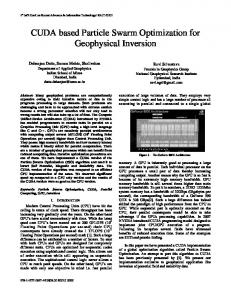
Similar to what happens in CSO, in the tracing mode of BCSO, cats are moving towards the best target. The main difference between CSO and BCSO is in the definition of velocity. In CSO velocity defines the difference between the current and previous position of a cat, but in BCSO the velocity vector changes its meaning to the probability of mutation in each dimension of a cat. The velocity vector which is now changes its meaning to probability of change is updated as follows. Two velocity vector one for each cats are defined as 1 and V 0 . V 0 is the probability of the bits of the particle to Vkd kd kd 1 is the probability that bits of particle change to zero while Vkd change to one. Since in update equation of these velocities, which will be introduced later, the inertia term is used, these 1 and velocities are not complement. The update process of Vkd

(5)

1 and d 0 are updated as in (6). in which dkd kd 1 0 i f Xgbest,d = 1 T hen dkd = r1 c1 and dkd = −r1 c1 1 0 i f Xgbest,d = 0 T hen dkd = −r1 c1 and dkd = r1 c1

(6)

in which r1 has a random values in the interval of [0, 1], w is the inertia weight and c1 is a constant which is defined by the user. According to current position catk , the velocity of catk is calculated as: { 1 Vkd i f Xkd = 0 ′ Vkd (7) = 0 Vkd i f Xkd = 1 The probability of mutation in each dimension is defined by the parameter t which is calculated using the following equation. ′ tkd = sig(Vkd )=

1 ′

1 + e−Vkd

(8)

In which tkd takes a value in the interval of [0, 1]. Based on the value of tkd the new position of each dimension of cat is updated as follows. { xkd =

B. Tracing Mode

d = 1, ..., M

Xgbest,d xkd

i f rand < tkd d = 1, ..., M i f tkd < rand

(9)

′ It should be noted that the maximum velocity vector of Vkd ′ should be bounded to a value Vmax . If the value of Vkd becomes larger than Vmax , Vmax should be selected for velocity in the corresponding dimension. Fig. 3 depicts the flowchart of BCSO.

IV.

E XPERIMENTAL R ESULTS

The BCSO algorithm is simulated on a zero-one knapsack problem and a number of benchmark functions. All calculations are done using MatLab R2010a running on an Intel Corei5 with 4GB memory. The results obtained using BCSO are compared with that of Genetic Algorithm [14], and two versions of PSO [12], [13] are compared. The parameter of BCSO are selected as SMP = 3, CDC = 0.2, SPC = True

Fig. 3.

Flowchart of binary cat swarm optimization algorithm.

and PMO = 0.2. In order to have a better comparison, the simulations are performed in 10 independent runs. The average, standard deviations, best and worst results found in the simulations are reported.

f1 (x)

=

n

∑ xi2

(10)

i=1

A. test functions In this section we investigate our proposed method on the minimization of test functions set which are used commonly in the literature. The test functions used here are: Sphere, Rastrigin, Ackley and Rosenbrock which are represented in equation (10)-(13). The global minimum of all of these functions is zero. The expression of these test functions are as follows.

f2 (x) f3 (x)

n

= 10n + ∑ xi2 − 10cos(2π xi ) (11) i=1 √ 1 n 2 1 n = −20exp(−0.2 x ) − exp( ∑ i ∑ cos(2π xi )) n i=1 n i=1 + 20 + exp(1)

f4 (x)

=

(12)

n−1

∑ [100(xi+1 − xi2 )2 + (xi − 1)2 ]

i=1

(13)

In this experiments 20 bits are used to represent binary values for the real numbers. Population size is 100, the number of iteration is 500, Dimension of the input space is 20 and Range of the particles are set to [-50, 50]. The results of solving the test functions are shown in Table I. Table I. summarizes the results of applying four different optimization methods to benchmark problems in terms of mean value, standard deviation, the best result found and the worst results. As can be seen from the table, the proposed method outperforms BPSO, NBPSO and GA considerably. In addition the convergence trend of the proposed method is compared with that of BPSO, NBPSO and GA on Rastrigin function, Rosenbrock function and Sphere function and are presented in Fig. 5, Fig. 6 and Fig. 7 respectively. These figures show that the proposed BCSO converges much faster than above mentioned algorithms. B. Zero-one knapsack problem

n

max f (x) = ∑ bi xi

(14)

i=1

n

∑ ri xi ≤ α

i = 1, 2, ..., n

i=1

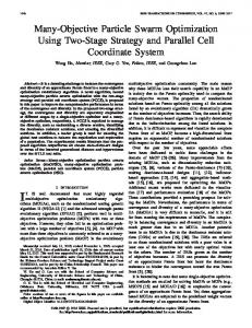
Let there be n items, x1 to xn where xi have a value bi and weight ri . The maximum weight that we can carry in the bag is α . It is common to assume that all values and weights are nonnegative. In this simulation we used random integers of the interval of [1, 15] as the weights and values of each item. The results of solving the knapsack problem are shown in Table II in terms of mean value, standard deviation, best value and worst value in 10 times of run of the simulation with different starting points. As can be seen from the table BCSO outperforms BPSO, NBSPO and GA. Figure 4 shows the trends of different optimization algorithms for solving the knapsack problem with 400 items and 1500 Iteration. As can be seen from the figure, BCSO converges much faster than other mentioned optimization algorithms. V.

T HE RESULTS OF APPLYING DIFFERENT OPTIMIZATION ALGORITHMS TO THE MINIMIZATION OF BENCHMARK FUNCTIONS

function sphere

rastrigin

ackley

rosenbrock

Result mean std best worst mean std best worst mean std best worst mean std best worst

Binary cat 9.559E-06 1.832E-05 4.547E-08 4.767E-05 62.926 14.477 39.247 85.536 0.520 0.076 0.396 0.622 978.645 906.829 53.078 2535.926

BPSO [12] 4069.325 521.741 3450.172 4985.068 4427.068 344.204 3949.418 5108.891 2.278 0.016 2.247 2.298 183591333.6 52644778.07 82596214.35 261891281

BPSO [13] 253.726 78.870 125.292 411.183 405.578 61.063 290.560 482.262 2.440 0.006 2.432 2.448 974594.660 791245.182 176676.042 2643866.996

Ga [14] 226.251 120.151 72.408 404.530 426.687 158.943 230.027 688.226 1.341 0.102 1.211 1.479 936010.460 645696.927 440545.444 2684943.349

R EFERENCES

The knapsack problem is a problem in combinatorial optimization. In this problem it is assumed that there are multiple items on hand each with a specific value and weight. The goal of this problem is to maximize the total value while the total weight is less than or equal to a given limit [15], [16]. The Zero-one knapsack problem can be mathematically formulated as follows.

sub ject to

TABLE I.

C ONCLUSION

In this paper, a new binary discrete optimization algorithm based on behavior of group of cats is presented. In binary discrete optimization problems the position vector are binary zero and one values. This causes significant change in BCSO with respect to CSO. In fact in BCSO in the seeking mode the slight change in the position takes place by introducing the mutation operation. The interpretation of velocity vector in tracing mode also changes to probability of change in each dimension of position of the cats. The proposed BCSO is implemented and tested on zero-one knapsack problem and a number of different benchmark problems. The obtained results are compared with that of BPSO, NBPSO and GA. The simulation results shows the proposed method greatly outperforms the above mentioned algorithms in terms of accuracy of the obtained results and speed of convergence.

[1] S. Sra, S. Nowozin, and S. J. Wright, Optimization for Machine Learning. Mit Pr, 2012. [2] K. Deb, “An introduction to genetic algorithms,” Sadhana, vol. 24, no. 4-5, pp. 293–315, 1999. [3] R. Eberhart and J. Kennedy, “A new optimizer using particle swarm theory,” in Micro Machine and Human Science, 1995. MHS’95., Proceedings of the Sixth International Symposium on. IEEE, 1995, pp. 39–43. [4] J. Kennedy and R. Eberhart, “Particle swarm optimization,” in Neural Networks, 1995. Proceedings., IEEE International Conference on, vol. 4. IEEE, 1995, pp. 1942–1948. [5] S.-C. Chu, P.-W. Tsai, and J.-S. Pan, “Cat swarm optimization,” in PRICAI 2006: Trends in Artificial Intelligence. Springer, 2006, pp. 854–858. [6] M. Khanesar, M. Shoorehdeli, and M. Teshnehlab, “Hybrid training of recurrent fuzzy neural network model,” in Mechatronics and Automation, 2007. ICMA 2007. International Conference on. IEEE, 2007, pp. 2598–2603. [7] M. A. Khanesar, M. Teshnehlab, E. Kayacan et al., “A novel type2 fuzzy membership function: Application to the prediction of noisy data,” in Computational Intelligence for Measurement Systems and Applications (CIMSA), 2010 IEEE International Conference on. IEEE, 2010, pp. 128–133. [8] D. Van der Merwe and A. Engelbrecht, “Data clustering using particle swarm optimization,” in Evolutionary Computation, 2003. CEC’03. The 2003 Congress on, vol. 1. IEEE, 2003, pp. 215–220. [9] J.-B. Park, Y.-M. Park, J.-R. Won, and K. Y. Lee, “An improved genetic algorithm for generation expansion planning,” Power Systems, IEEE Transactions on, vol. 15, no. 3, pp. 916–922, 2000. [10] S.-C. Chu and P.-W. Tsai, “Computational intelligence based on the behavior of cats,” International Journal of Innovative Computing, Information and Control, vol. 3, no. 1, pp. 163–173, 2007. [11] A. P. Engelbrecht, Fundamentals of computational swarm intelligence. Wiley Chichester, 2005, vol. 1. [12] J. Kennedy and R. C. Eberhart, “A discrete binary version of the particle swarm algorithm,” in Systems, Man, and Cybernetics, 1997. Computational Cybernetics and Simulation., 1997 IEEE International Conference on, vol. 5. IEEE, 1997, pp. 4104–4108. [13] M. A. Khanesar, M. Teshnehlab, and M. A. Shoorehdeli, “A novel binary particle swarm optimization,” in Control & Automation, 2007. MED’07. Mediterranean Conference on. IEEE, 2007, pp. 1–6. [14] J. Sadri and C. Y. Suen, “A genetic binary particle swarm optimization model,” in Evolutionary Computation, 2006. CEC 2006. IEEE Congress on. IEEE, 2006, pp. 656–663. [15] S. Martello and P. Toth, Knapsack problems: algorithms and computer implementations. John Wiley & Sons, Inc., 1990. [16] D. Pisinger, “Where are the hard knapsack problems?” Computers & Operations Research, vol. 32, no. 9, pp. 2271–2284, 2005.

TABLE II.

T HE RESULTS OF APPLYING FOUR DIFFERENT OPTIMIZATION ALGORITHMS TO THE MAXIMIZATION OF ZERO - ONE KNAPSACK PROBLEM Population size

Number of item

Maximum Weight backpack

Maximum iteration

30

75

50

1000

30

100

85

1000

40

200

170

1000

50

400

160

1500

Result

BCSO

BPSO [12]

BPSO [13]

Ga [14]

mean std best worst mean std best worst mean std best worst mean std best worst

163.200 2.683 167.000 161.000 232.800 3.899 238.000 229.000 356.600 10.854 368.000 344.000 585.000 21.703 599.000 560.000

2.348 0.264 2.634 2.022 2.240 0.105 2.360 2.123 1.657 0.029 1.691 1.621 1.371 0.021 1.393 1.351

158.200 3.421 162.000 153.000 218.000 8.426 227.000 207.000 167.223 144.766 312.000 6.667 2.537 0.033 2.559 2.499

152.800 4.147 157.000 147.000 210.200 4.919 216.000 203.000 73.273 141.877 327.000 7.250 2.321 0.206 2.516 2.106

3

9

10

10

8

10 binary CSO binary PSO [12] binary PSO [13] binary GA [14]

7

10

6

10 Cost

Value Backpack

2

10

5

10

binary CSO binary PSO [12] binary PSO [13] binary GA [14]

1

10

4

10

3

10 0

10

2

0

500

1000

10

1500

0

200

400

Iteration

600

800

1000

Iteration

Fig. 4. The convergence trend of four different optimization algorithms when they are applied to maximization of zero-one knapsack problem

Fig. 6. The convergence trend of four different optimization algorithms when they are applied to minimization of Rosenbrock function

4

4

10

10

2

10 3

10

0

Cost

Cost

10

−2

10 2

10

binary CSO binary PSO [12] binary PSO [13] binary GA [14] 1

10

0

binary CSO binary PSO [12] binary PSO [13] binary GA [14]

−4

10

−6

200

400

600

800

1000

Iteration

Fig. 5. The convergence trend of four different optimization algorithms when they are applied to minimization of Rastrigin function

10

0

200

400

600

800

1000

Iteration

Fig. 7. The convergence trend of four different optimization algorithms when they are applied to minimization of sphere function