Hagen [29] .... Similarly, to minimize with respect to the control input k ...... system critic network converges to the solution of the ARE, and the actor network.
DISCRETE-TIME CONTROL ALGORITHMS AND ADAPTIVE INTELLIGENT SYSTEMS DESIGNS
by
ASMA AZMI AL-TAMIMI
Presented to the Faculty of the Graduate School of The University of Texas at Arlington in Partial Fulfillment of the Requirements for the Degree of
DOCTOR OF PHILOSOPHY
THE UNIVERSITY OF TEXAS AT ARLINGTON May 2007
Copyright © by Asma Al-Tamimi 2007 All Rights Reserved
ACKNOWLEDGEMENTS
I would like to express my sincere thanks to my supervisor Professor Frank L. Lewis for his supervision and guidance during my doctoral research work. I also extend my thanks to Dr. Murad Abu-Khalaf for his close instrumental supervision during my research work at ARRI. My thanks also go to my defense committee: Kai-Shing Yeung, Wei-Jen Lee, Dan Popa, and Kamesh Subbarao for their time, suggestions, and remarks to improve this work. Moreover, I like to thank my colleagues in the ACS group and every one else who helped me during my studies in the USA. I would like to acknowledge the financial support of the Hashemite University. I also acknowledge the financial support by the Electrical Engineering Department, and the Automation Robotics Research Institute. The research in this dissertation was funded by the National Science Foundation ECS-0501451 and the Army Research Office W91NF-05-1-0314. I am very indebted to my parents for their infinite support, care and attention without which I would have not been at this stage in my life. I have been greatly inspired by them and I dedicate this dissertation to my mother Khawla and father Azmi. March 30, 2007 iii
ABSTRACT
DISCRETE-TIME CONTROL ALGORITHMS AND ADAPTIVE INTELLIGENT SYSTEMS DESIGNS Publication No. ______
Asma Azmi Al-Tamimi, PhD.
The University of Texas at Arlington, 2007
Supervising Professor: Frank L. Lewis In this work, approximate dynamic programming (ADP) designs based on adaptive critic structures are developed to solve the discrete-time H 2 / H ∞ optimal control problems in which the state and action spaces are continuous. This work considers linear discrete-time systems as well as nonlinear discrete-time systems that are affine in the input. This research resulted in forward-in-time reinforcement learning algorithms that converge to the solution of the Generalized Algebraic Riccati Equation (GARE) for linear systems. For the nonlinear case, a forward-in-time reinforcement learning algorithm is presented that converges to the solution of the associated Hamilton-Jacobi Bellman equation (HJB).
iv
The results in the linear case can be thought of as a way to solve the GARE of the well-known discrete-time H ∞ optimal control problem forward in time. Four design algorithms are developed: Heuristic Dynamic programming (HDP), Dual Heuristic dynamic programming (DHP), Action dependent Heuristic Dynamic programming (ADHDP) and Action dependent Dual Heuristic dynamic programming (ADDHP). The significance of these algorithms is that for some of them, particularly the ADHDP algorithm, a priori knowledge of the plant model is not required to solve the dynamic programming problem. Another major outcome of this work is that we introduce a convergent policy iteration scheme based on the HDP algorithm that allows the use of neural networks to arbitrarily approximate for the value function of the discrete-time HJB equation. This online algorithm may be implemented in a way that requires only partial knowledge of the model of the nonlinear dynamical system. The dissertation includes detailed proofs of convergence for the proposed algorithms, HDP, DHP, ADHDP, ADDHP and the nonlinear HDP. Practical numerical examples are provided to show the effectiveness of the developed optimization algorithms. For nonlinear systems, a comparison with methods based on the StateDependent Riccati Equation (SDRE) is also presented. In all the provided examples, parametric structures like neural networks have been used to find compact representations of the value function and optimal policies for the corresponding optimal control problems.
v
TABLE OF CONTENTS
ACKNOWLEDGEMENTS.......................................................................................
iii
ABSTRACT ..............................................................................................................
iv
LIST OF ILLUSTRATIONS.....................................................................................
ix
Chapter 1. INTRODUCTION.........................................................................................
1
2. DISCRETE-TIME H-INFINITY STATE FEEDBACK CONTROL FOR ZERO-SUM GAMES .......................................................
5
3. HEURISTIC DYNAMIC PROGRAMMING H-INFINTY CONTROL DESIGN.....................................................................................
14
3.1. Heuristic Dynamic Programming (HDP) ...............................................
14
3.1.1. Derivation of HDP for zero-sum game....................................
15
3.1.2. Online Implementation of the HDP Algorithm .......................
17
3.1.3. Convergence of the HDP Algorithm .......................................
20
3.2. Dual Heuristic Dynamic Programming (DHP).......................................
22
3.2.1. Derivation of DHP for Zero-Sum Games ...............................
23
3.2.2. Online Implementation of the DHP Algorithm .......................
26
3.2.3. Convergence of the DHP Algorithm .......................................
29
3.3. Online ADP H ∞ Autopilot Controller Design for an F-16 aircraft .......
31
3.3.1. H ∞ Solution Based on the Riccati Equation.........................
32
vi
3.3.2. HDP based H ∞ Autopilot Controller Design .........................
33
3.3.3. DHP based H ∞ Autopilot Controller Design .........................
38
3.4. Conclusion ..............................................................................................
43
4. ACTION DEPENDENT HEURISTIC DYNAMIC PROGRAMMING H-INFINTY CONTROL DESIGN................................................................
44
4.1 Q-Function Setup for Discrete-Time Linear Quadratic Zero-sum Games.......................................................................................
44
4.2. Action Dependent Heuristic Dynamic Programming (ADHDP) ...........
50
4.2.1. Derivation of the ADHDP for the Zero-Sum Games ..............
51
4.2.2. Online Implementation of the ADHDP algorithm...................
55
4.2.3. Convergence of the ADHDP Algorithm..................................
58
4.3. Action Dependent Dual Heuristic Dynamic Programming (ADDHP)...
61
4.3.1. Derivation of the ADDHP Algorithm......................................
62
4.3.2. Online Implementation for the ADDHP algorithm .................
67
4.3.3. Convergence of the ADDHP Algorithm..................................
70
4.4. Online ADP H ∞ Autopilot Controller Design for an F-16 Aircraft ......
74
4.4.1. H ∞ Solution Based on the Riccati Equation..........................
75
4.4.2. ADHDP based H ∞ Autopilot Controller Design ....................
76
4.4.3. ADDHP based H ∞ Autopilot Controller Design ....................
81
4.5. Conclusion ..............................................................................................
84
5. APPLICATION OF THE ADHDP FOR THE POWER SYSTEM AND SYTEM IDENTIFICATION ..............................................
87
5.1. Power System Model Plant.....................................................................
87
vii
5.2. H-Infinity Control Design Using ADHDP Algorithm............................
89
5.3. System Identification ..............................................................................
94
5.4. Conclusion ..............................................................................................
97
6. NONLINEAR HEURISTIC DYNAMIC PROGRAMMING OPTIMAL CONTROL DESIGN ..................................................................
98
6.1. The Discrete-Time HJB Equation ..........................................................
98
6.2. The Nonlinear HDP Algorithm .............................................................. 100 6.3. Convergence of the HDP Algorithm ...................................................... 101 6.4. Neural Network Approximation ............................................................. 104 6.5. Discrete-time Nonlinear System Example.............................................. 108 6.5.1. Linear system example ............................................................ 108 6.5.2. Nonlinear System Example ..................................................... 111 6.5. Conclusion .............................................................................................. 115 7. CONCLUSION AND FUTURE WORK...................................................... 116 REFERENCES .......................................................................................................... 119 BIOGRAPHICAL INFORMATION......................................................................... 123
viii
LIST OF ILLUSTRATIONS Figure
Page
3.1
The HDP Algorithm ........................................................................................ 20
3.2
The DHP Algorithm ........................................................................................ 28
3.3
The convergence of Pi by iterating on the Riccati equation........................... 32
3.4
State trajectories with re-initialization for the HDP algorithm ....................... 34
3.5
The control and the disturbance in the HDP ................................................... 35
3.6
Convergence of the critic network parameters in the HDP............................. 36
3.7
Convergence of the disturbance action network parameters in the HDP........ 37
3.8
Convergence of the control action network parameters in the HDP............... 37
3.9
State trajectories with re-initialization for the DHP algorithm ....................... 39
3.10
The control and the disturbance in the DHP ................................................... 39
3.11
Convergence of the critic network parameters in the DHP............................. 40
3.12
Convergence of the disturbance action network parameters in the DHP........ 41
3.13
Convergence of the control action network parameters in the DHP............... 41
4.1
The ADHDP algorithm ................................................................................... 57
4.2
The ADDHP algorithm ................................................................................... 69
4.3
The convergence of Pi by iterating on the Riccati equation........................... 75
4.4
State trajectories in the ADHDP algorithm..................................................... 77
4.5
The control and disturbance in the ADHDP ................................................... 78 ix
4.6
Convergence of Pi in the ADHDP.................................................................. 79
4.7
Convergence of the disturbance action network parameters in the ADHDP.. 80
4.8
Convergence of the control action network parameters in the ADHDP ......... 80
4.9
State trajectories in the ADDHP ..................................................................... 81
4.10
The control and the disturbance in the ADDHP ............................................. 82
4.11
Convergence in the Pi in the ADDHP ............................................................ 83
4.12
Convergence of the disturbance action network parameters in the ADDHP.. 83
4.13
Convergence of the control action network parameters in the ADDHP ......... 84
5.1
The Convergence of Pi → P .......................................................................... 90
5.2
The Convergence of the control policy........................................................... 91
5.3
The states trajectories for the system with the H ∞ controller ........................ 92
5.4
The states trajectories for the system with the controller designed in [33] .... 93
5.5
The states trajectories for the system with the H ∞ controller ....................... 93
5.6
The states trajectories for the system with the controller designed in [33]..... 94
6.1
The nonlinear HDP algorithm......................................................................... 107
6.2
The state trajectories ( x1 ) for both methods ................................................... 113
6.3
The state trajectories ( x2 ) for both methods ................................................... 113
6.4
The cost function for both methods ................................................................ 114
6.5
The control input for both methods................................................................. 114
x
CHAPTER 1 INTRODUCTION
In this dissertation, adaptive critic designs that are based on the dynamic programming principle are developed to solve H 2 / H ∞ optimal control problems for discrete-time dynamical systems. In the case of H ∞ optimal control, the zero-sum game for discrete-time linear systems is solved by creating and developing adaptive critic structures that learn to co-exist. In the H 2 optimal control case, the dynamical programming problem associated with nonlinear discrete-time dynamical systems is solved, i.e. solving for the value function of the corresponding HJB equation. Approximate dynamic programming, also known as Neuro Dynamic Programming, was first proposed by Werbos [27], Barto et. al. [1], Widrow et. al. [5], Howard [28], Watkins [8], Bertsekas and Tsitsiklis [11], and others to solve optimal control problems forward-in-time. The optimal control law, i.e. the action network, and the value function, i.e. the critic network, are modeled as parametric structures, i.e. neural networks. This is combined with incremental optimization such as reinforcement learning to tune and improve both networks forward-in-time and hence can be implemented in actual control systems. This overcomes computational complexity associated with dynamic programming, which is an offline technique that requires a backward-in-time solution procedure [15]. Moreover, as will be discussed in the 1
dissertation, some of the presented adaptive critic designs do not require the plant model for tuning the action network, the critic network, or both of them. Several approximate dynamic programming schemes appear in literature. Howard [28] proposed iterations in the policy space in the framework of stochastic decision theory. In [30], Bradtke et al. implemented a Q-learning policy iteration method for the discrete-time linear quadratic optimal control problem. Hagen [29] discussed the relation between the Q-learning policy iteration method and model-based adaptive control with system identification. Werbos [25] classified approximate dynamic programming approaches into four main schemes: Heuristic Dynamic Programming (HDP), Dual Heuristic Dynamic Programming (DHP), Action Dependent Heuristic Dynamic Programming (ADHDP), also known as Q-learning [8], and Action Dependent Dual Heuristic Dynamic Programming (ADDHP). In [9], Prokhorov and Wunsch developed new approximate dynamic programming schemes known as Globalized Dual Heuristic Dynamic Programming (GDHP) and Action Dependent Globalized Dual Heuristic Dynamic Programming (ADGDHP). Landelius [31] applied HDP, DHP, ADHDP and ADDHP techniques to the discrete-time linear quadratic optimal control problem and discussed their convergence showing that they are equal to iterating on the underlying Riccati equation. The current status of work on approximate dynamic programming is given in [20]. See also [11]. Reinforcement learning methods to solve game theory problems have recently appeared in [24] and [18] in the framework of Markov games where multiagent Qlearning methods are proposed and shown to converge to the Nash equilibrium under 2
specific conditions. Unlike the work in this dissertation, these are lookup-table-based methods concerned with discrete state and action spaces. In this dissertation, adaptive critic designs, namely HDP, DHP, ADHDP and ADDHP, are derived to solve dynamic programming problems online for discrete-time dynamical systems with continuous state and action spaces. Offline solutions of these optimal control problems based on the dynamic programming principle appear in [7], [6], [15]. An off-line neural net policy iterations solution based on the dynamic programming principle appears in [23] for the continuous-time case. The importance of this dissertation stems from the fact adaptive critics algorithms are used to design H 2 / H ∞ controller without knowing the dynamics of linear systems, e.g. ADHDP algorithm, and partial knowledge of the dynamics of nonlinear systems, e.g. HDP algorithm. Therefore, these algorithms may be thought of as being direct adaptive optimal control architectures. The organization of this dissertation is as follows. In Chapter 2, zero-sum games for discrete-time linear systems with quadratic infinite horizon cost are revisited. Dynamic programming is used to derive the optimal policies for both the control and the disturbance inputs along with the associated Riccati equation. Although equivalent to those found in literature [6], the derived policies are different in structure and appear in a form required for the design of adaptive critics. In Chapter 3, Heuristic Dynamic Programming (HDP) and Dual Heuristic Dynamic Programming (DHP) algorithms are proposed to solve the zero-sum game for linear systems forward-in-time. Chapter 4 extends the results of Chapter 3 to Action Dependent Heuristic Dynamic Programming 3
(ADHDP) and Action Dependent Dual Heuristic Dynamic Programming (ADDHP). In Chapter 5, an application of the ADHDP algorithm to the design of load frequency control systems is demonstrated. In Chapter 6 the nonlinear HDP algorithm is derived, with proofs of convergence, to solve for the HJB equation. It is also shown that the optimal controller derived through the DT HJB outperforms that using the State Dependent Riccati Equation (SDRE).
4
CHAPTER 2 DISCRETE-TIME H-INFINITY STATE FEEDBACK CONTROL FOR ZERO-SUM GAMES
In this chapter, the solution of the zero-sum game of a linear discrete-time system with quadratic cost derived under state feedback information structure. The policies for each of the two players, control and disturbance, are derived with the associated Riccati equation. Specific forms for both the Riccati equation and the control and disturbance policies are derived that are required for applications in ADP these forms are not same as standard forms in the existing literature. The relation between the derived policies and the associated Riccati equation with those existing in literature is discussed Consider the following discrete-time linear system xk +1 = Axk + Buk + Ewk yk = xk ,
.
(2.1)
where x ∈ R n , y ∈ R p , uk ∈ R m1 is the control input and wk ∈ R m2 is the disturbance input. Consider the infinite-horizon cost function. For any stabilizing sequence of policies uk and wk , one can write the infinite-horizon cost-to-go as V ( xk ) = ∑ i = k xiT Qxi + uiT ui − γ 2 wiT wi ∞
= xkT Qxk + ukT uk − γ 2 wkT wk + ∑ i = k +1 xiT Qxi + uiT ui − γ 2 wiT wi ∞
= xkT Qxk + ukT uk − γ 2 wkT wk + V ( xk +1 ) = r ( xk , uk , wk ) + V ( xk +1 ).
5
(2.2)
It is desired to find the optimal control uk∗ and the worst case disturbance wk∗ , in which the infinite-horizon cost is to be minimized by player 1, uk , and maximized by player 2, wk . Here the class of strictly feedback stabilizing policies is considered [6]. V ∗ ( xk ) = min max ∑ i = k xiT Qxi + uiT ui − γ 2 wiT wi ∞
u
w
(2.3)
Using the dynamic programming principle, the optimization problem in equation (2.3) and (2.2) can be written as
V ∗ ( x) = min max(r ( xk , uk , wk ) + V ∗ ( xk + )) u
w
= max min(r ( xk , uk , wk ) + V ∗ ( xk + )). w
(2.4)
u
If we assume that there exists a solution to the GARE that is strictly feedback stabilizing, then it can be shown, see[10], that the policies are in saddle-point equilibrium, i.e. minimax is equal to maximin, in the restricted class of feedback stabilizing policies under which xk → 0 as k → ∞ for all x0 ∈ R n . See [6], p. 340), and ( [7], p. 138) and [13][10]. It is known that the optimal cost is quadratic in the state, and it is given as V ∗ ( xk ) = xkT Pxk
(2.5)
where P ≥ 0 . Assuming that the game has a value and is solvable, then in order to have a unique feedback saddle-point in the class of strictly feedback stabilizing policies, the inequalities in (2.6) and (2.7) should be satisfied, [7], I − γ −2 E T PE > 0
6
(2.6)
I + BT PB > 0 .
(2.7)
Applying the Bellman optimality principle, one has V ∗ ( xk ) = minmax(r ( xk , uk , wk ) + V ∗ ( xk +1 )) u
w
= minmax( xkT Qxk + ukT uk − γ ^ 2 wkT wk + xkT+1 Pxk +1 ). u
(2.8)
w
Substituting (2.5) in equation(2.8) one has xkT Pxk = minmax( xkT Qxk + ukT uk − γ ^ 2 wkT wk u
w
+ ( Axk + Buk + Ewk )T P ( Axk + Bu k + Ewk ).
(2.9)
To maximize with respect to the disturbance wk , one needs to apply the first order necessary condition ∂Vk =0 ∂wk
(2.10) 2
T
= −2γ wk + 2 E P ( A + Buk + Ewk ).
Therefore, the disturbance can be written as wk = (γ 2 I − E T PE ) −1 ( E T PAxk + E T PBuk ) .
(2.11)
Similarly, to minimize with respect to the control input uk one has ∂Vk =0 ∂uk
(2.12)
= 2uk + 2 BT P ( A + Buk + Ewk ).
Hence, the controller can be written as uk = −( I + BT PB ) −1 ( BT PAxk + BT PEwk ) .
(2.13)
Note that applying the 2nd order sufficiency conditions for both players, one obtains (2.6) and (2.7). Substituting equation (2.11) in (2.12) 7
uk∗ = ( I + BT PB − BT PE ( E T PE − γ 2 I ) −1 E T PB) −1 ×
,
(2.14)
.
(2.15)
( BT PE ( E T PE − γ 2 I ) −1 E T PA − BT PA) xk so the optimal control is a state feedback with gain
L = ( I + BT PB − BT PE ( E T PE − γ 2 I ) −1 E T PB) −1 × ( BT PE ( E T PE − γ 2 I ) −1 E T PA − BT PA).
Substituting the equation (2.13) in (2.10) one can find the optimal policy to the disturbance
wk∗ = ( E T PE − γ 2 I − E T PB ( I + BT PB)−1 BT PE ) −1 × ( BT PE ( I + BT PB) −1 BPA − E T PA) xk
,
(2.16)
so the optimal disturbance is a state feedback with gain
K = ( E T PE − γ 2 I − E T PB( I + BT PB) −1 BT PE )−1 × ( E T PB( I + BT PB) −1 BPA − E T PA).
(2.17)
Note that the inversion matrices in (2.14) and (2.16) exists due to (2.6) and (2.7) It is now going to be shown that the policies obtained in equations (2.15) and (2.17) are equivalent to those known in the literature [7]. The following Lemma is required.
Lemma 2.1: If ( I − γ −2 E T PE ) is invertible, then ( I − γ −2 EE T P ) is also invertible. Proof: Since ( I − γ −2 E T PE ) is invertible then the following expression is valid I + γ −2 E ( I − γ −2 E T PE ) −1 E T P .
Applying the matrix inversion lemma, [15], it can be shown that I + γ −2 E ( I − γ −2 E T PE ) −1 E T P = ( I − γ −2 EE T P ) −1
Hence, I − γ −2 EE T P is invertible and I − γ −2 EE T P > 0 .
8
□
Lemma 2.2: The optimal policies for control L , and disturbance K , in equation (2.15) and (2.17) respectively are equivalent to the ones that appear in [7], namely
L = − BT P( I − BBT P − γ 2 EE T P)−1 ) A K = −γ −2 E T P( I − BBT P − γ 2 EE T P)−1 ) A. Proof: To show the control policy part, L , one can rewrite (2.15) as follows
L = ( I + BT P( I − E ( E T PE − γ 2 I ) −1 E T P) B) −1 × BT P( E ( E T PE − γ 2 I ) −1 E T P − I ) A.
(2.18)
Applying the well known matrix inversion lemma, [15], on the (2.18), one has L = −( I + BT P ( I − γ 2 EE T P ) −1 B ) −1 BT P ( I − γ −2 EE T P ) −1 A .
(2.19)
Note that ( I − γ 2 EE T P ) is invertible due to lemma 2.1. Applying the matrix inversion lemma on (2.19), one has L = −( I − BT P ( BBT P + I − γ 2 EE T P ) −1 B ) BT P ( I − γ −2 EE T P )−1 A.
(2.20)
One can rewrite equation (2.20) as follows L = − BT P ( I − ( BBT P + I − γ 2 EE T P ) −1 BBT P ) × ( I − γ −2 EE T P ) −1 A .
(2.21)
Applying the matrix inversion lemma on (2.21), one has L = − BT P ( I + BBT P − γ 2 EE T P )−1 ) A .
(2.22)
Note that since I − γ −2 EE T P > 0 , then I + BBT P − γ 2 EE T P > 0 and concludes that equation (2.22) is equivalent to the control policy that appears on [7]. To show the control policy part, K , one can rewrite (2.17) as follows K = (−γ 2 I + E T P ( E − B ( I + BT PB ) −1 BT P ) E )−1 × E T P ( B ( I + BT PB ) −1 BP − I ) A .(2.23)
Applying the matrix inversion Lemma on (2.23), on has
9
K = −(−γ 2 I + E T P ( I + BBT P ) −1 E )−1 E T P ( I + BBT P ) A .
(2.24)
Applying the matrix inversion lemma on equation (2.24), one has K = γ −2 ( I + γ −2 E T P ( BBT P + I − γ 2 EE T P ) −1 E ) E T P × ( I + BBT P )−1 A .
(2.25)
One can rewrite (2.25) as follows K = γ −2 E T P ( I + ( BBT P + I − γ 2 EE T P ) −1 γ −2 EE T P ) × ( I + BBT P ) −1 A .
(2.26)
Applying the matrix inversion lemma on equation (2.26), one obtains K = γ −2 E T P ( I + BBT P − γ 2 EE T P ) −1 ) A .
(2.27)
Note that since I − γ −2 EE T P > 0 , then I + BBT P − γ 2 EE T P > 0 and concludes that equation (2.27) is equivalent to the disturbance policy that appears in [7].
Next it is shown that the value function of the game V ∗ ( xk ) = xkT Pxk satisfies a Riccati equation. The form of the Riccati equation derived in this chapter, under state feedback information structure in order to perform ADP. It is similar to the one appearing in [3] which was derived under full information structure. Moreover, it will be shown that the Riccati equation derived in this chapter is equivalent to the work in [7] derived under the same state feedback information structure. Note that (2.9) can be rewritten as follows xkT Pxk = ( xkT Qxk + u ∗Tk u ∗k − γ 2 w∗Tk w∗k + ( Axk + Bu ∗k + Ew∗k )T P ( Axk + Bu ∗ k + Ew∗ k )) .(2.28)
This is equivalent
P = Q + LT L − γ 2 K T K + ( A + BL + EK )T P( A + BL + EK )) = Q + LT L − γ 2 K T K + Acl T PAcl . where Acl = A + BL + EK . Equation (2.29) is the closed-loop Riccati equation.
10
(2.29)
Next it is shown upon substituting (2.15) and (2.17) in (2.29), one obtains the desired Riccati equation upon which the adaptive critic designs are based.
Lemma 2.3: Substituting the policies, (2.15) and (2.17), in (2.29) one can obtain the Riccati equation that appears in [3][34], and given by −1
T
I + BT PB BT PE BT PA A PE ] T T . T 2 E PB E PE − γ I E PA
T
T
P = A PA + Q − [ A PB
Proof: The control policy and the disturbance policy can be written as follows L = D11−1 ( A12 A22−1 E T PA − BT PA) ,
(2.30)
K = D22−1 ( A21 A11−1 BT PA − E T PA),
(2.31)
where
D11−1 = ( I + BT PB − BT PE ( E T PE − γ 2 I ) −1 E T PB ) −1 A12 = BT PE A21 = E T PB A11 = I + BT PB A22 = E T PE − γ 2 I D22−1 = ( E T PE − γ 2 I − E T PB ( I + BT PB ) −1 BT PE ) −1. From (2.6) and (2.7), one concludes that D11−1 and D22−1 are invertible. Equations (2.30) and (2.31) can be written as follows
D11−1 L K = − −1 −1 D22 A21 A22
− D11−1 A12 A22−1 BT PA T . D22−1 E PA
It is known that, [15], A11 A 21
−1
A12 D11−1 = −1 −1 A22 D22 A21 A22 11
− D11−1 A12 A22−1 . D22−1
(2.32)
Therefore one can rewrite (2.32) as follows
A11 L = − A K 21
−1
−1
A12 BT PA I + BT PB BT PE BT PA = − T . A22 E T PA E T PE − γ 2 I E T PA E PB
(2.33)
Equation (2.29) can be written as follows P = ( A + BL + EK )T P ( A + BL + EK ) + LT L − γ 2 K T K + Q = AT PA + AT PBL + AT PEK + LT BT PA + K T E T PA + LT
BT PB K T T E PB
BT PE L T + L E T PE K
(2.34)
0 L I K T + Q. 2 0 −γ I K
Substituting (2.33) in (2.34), one has P = AT PA + AT PBL + AT PEK + LT BT PA + K T E T PA I + BT PB BT PE I + BT PB − L K T E T PE − γ 2 I E T PB E PB = AT PA + AT PBL + AT PEK + Q. T
T
−1
BT PA + Q .(2.35) E T PE − γ 2 I E T PA BT PE
Equation (2.35) can be written as P = AT PA + AT PB
L AT PE + Q. K
(2.36)
Substituting (2.32) in (2.36), one has the desired Riccati equation −1
T
T
P = A PA + Q − [ A PB
I + BT PB BT PE BT PA A PE ] T E T PE − γ 2 I E T PA E PB T
It can be seen that (2.37) is the Riccati equation that appears in [3][34][32].
(2.37)
It is shown in [3] that (2.37) is equivalent to the Riccati equation that appears in [7] and [6], which is given as P = Q + AT P ( I + ( BBT − γ −2 EE T ) P ) −1 A . It is important to note that the H 2 problem is a special case of the H ∞ where in the system equation, (2.1) , E = 0 or in the value function,(2.2) , γ → ∞ , i.e. P will be
12
the solution of the discrete-time algebraic Riccati equation DARE. One form of the DARE is P = AT PA + Q − AT PB ( I + BT PB ) −1 BT PA
13
CHAPTER 3 HUERISTC DYNAMIC PROGRAMING H-INFINTY COTROL DESIGN
In this chapter, adaptive critic approximate dynamic programming designs are derived to solve the discrete-time zero-sum game in which the state and action spaces are continuous. This results in a forward-in-time reinforcement learning algorithm that converges to the Nash equilibrium of the corresponding zero-sum game. The results in this chapter can be thought of as a way to solve the Riccati equation of the well-known discrete-time H ∞ optimal control problem forward in time. Two schemes are presented, a Heuristic Dynamic Programming (HDP) and a Dual Heuristic Dynamic Programming (DHP) to solve for the value function and the co-state of the game respectively. An H ∞ autopilot design for an F-16 aircraft is presented to illustrate the results 3.1 Heuristic Dynamic Programming (HDP) In this section, an HDP algorithm is developed to solve the discrete-time linear system zero-sum game described in chapter 2. The HDP algorithm was originally proposed in [25] to solve optimal control problems. The HDP algorithm has been applied earlier to solve the discrete-time Linear Quadratic Regulator (LQR) in optimal control theory [31]. In the HDP approach, a parametric structure is used to approximate the cost-to-go function of the current control policy. Then the certainty equivalence principle is used to improve the policy of the action network. 14
In this section, we extend the HDP approach to linear quadratic discrete-time zero-sum games appearing in [7], and prove the convergence of the presented algorithm. 3.1.1 Derivation of HDP for Zero-Sum Games Consider the system xk +1 = Axk + Buk + Ewk yk = xk ,
(3.1)
and the cost-to-go function as V ( xk ) = min max ∑ i = k xiT Qxi + uiT ui − γ 2 wiT wi ∞
u
w
(3.2)
The HDP is developed to solve the zero-sum game described in chapter 2, one starts with an initial cost-to-go V0 ( x) ≥ 0 that is not necessarily optimal, and then finds V1 ( x) by solving equation (3.3) with i = 0 according to Vi +1 ( xk ) = min max { xkT Qxk + ukT uk − γ 2 wkT wk + Vi ( xk +1 )} . uk
wk
(3.3)
Equation (3.3) is a recurrence relation that is used to solve for the optimal cost-to-go, the game value function, forward in time. Note that since Vi ( x) is not initially optimal, optimal policies found using Vi ( x) in (3.3) use the certainty equivalence principle and are denoted as ui ( xk ) and wi ( xk ) . Then, Vi +1 ( x) is given by Vi +1 ( xk ) = xkT Qxk + uiT ( xk )ui ( xk ) − γ 2 wiT ( xk ) wi ( xk ) + Vi ( xk +1 ) .
15
(3.4)
Once Vi +1 ( x) is found, one then repeats the same process for i = 0,1,2,… . In this chapter, it is shown that Vi +1 ( xk ) → V ∗ ( xk ) as i → ∞ , where V * ( xk ) is the optimal value function for the game based on the solution to the GARE (2.37). In the HDP approach, the cost-to-go function, Vi ( x) , is generally difficult to obtain in closed-form except in special cases. Therefore, in general a parametric structure Vˆ ( x, pi ) , is used to approximate the actual Vi ( x) . Similarly, parametric structures are used to obtain approximate closed-form representations of the two action networks uˆ( x, L) and wˆ ( x, K ) . Since in this chapter the zero-sum game considered is linear and quadratic, it is well-known that the cost-to-go function is quadratic in the state, i.e. V ( x) = xT Px , and the two action networks are linear in the state. Therefore a natural choice of these parameter structures is given as
Vˆ ( x, pi ) = piT x ,
(3.5)
uˆ ( x, Li ) = LTi x ,
(3.6)
wˆ ( x, K i ) = K iT x ,
(3.7)
where x = ( x12 ,… , x1 xn , x22 , x2 x3 ,… , xn −1 xn , xn2 ) , is the Kronecker product quadratic polynomial basis vector [21], and p = v( P ) , where v(⋅) is a vector function that acts on
n × n matrices and outputs a
n ( n+1) 2
× 1 column vector. The output vector of v(⋅) is
constructed by stacking the columns of the squared matrix into a one-column vector with the off-diagonal elements summed as Pij + Pji , [21]. The parameter structures (3.5) (3.6) and (3.7) give an exact closed-form representation of the functions in (3.4). 16
It can be shown that the parameters of the action networks, Li and K i of (3.6) and (3.7), are found as T −1 Li = ( I + BT PB − BT PE − γ 2 I )−1 E T PB i i ( E PE i i ) × T ( BT PE − γ 2 I ) −1 E T Pi A − BT Pi A), i ( E PE i T −1 T −1 K i = ( E T PE − γ 2 I − E T PB i i ( I + B PB i ) B PE i ) × T −1 T T ( E T PB i ( I + B PB i ) B Pi A − E Pi A).
(3.8)
(3.9)
These are greedy policy iterations that are based on the certainty equivalence principle when compared to (2.15) and (2.17), since they depend on Pi which does not necessarily solve (2.37). Note that to update the action networks, it is necessary to know the plant model A and B matrices. After determining (3.8) and (3.9) substituting them in (3.4), one then has d ( xk , pi ) = xkT Qxk + ( Li xk )T ( Li xk ) − γ 2 ( K i xk )T ( K i xk ) + piT xk +1
(3.10)
which can be thought of as the desired target function to which one needs to fit
Vˆ ( x, pi +1 ) in least-squares sense to find pi +1 such that piT+1 xk = d ( xk , pi )
(3.11)
The parameter vector pi +1 is found by minimizing the error between the target value function (3.10) and (3.11) in a least-squares sense over a compact set, Ω ,
pi +1 = arg min{∫ | piT+1 x − d ( x, pi ) |2 dx} . pi +1
(3.12)
Ω
3.1.2 Online Implementation of the HDP Algorithm The least-squares problem in (3.12) can be solved in real-time by collecting enough data points generated from d ( xk , pi ) in (3.10). This requires one to have 17
knowledge of the state information xk , xk +1 as the dynamics evolve in time, and also of the reward function r ( xk , uk , wk ) . This can be determined by simulation, or, in realtime applications, by observing the states on-line. Therefore, in the HDP algorithm, the model of the system is not needed to update the critic network, though it is needed to update the actions. To satisfy the excitation condition of the least-squares problem, one needs to have the number of collected points N at least N ≥ n(n + 1) / 2 , where n is the number of states. Therefore, after several time steps that are enough to guarantee the excitation condition, one has the following least-squares problem pi +1 = ( XX T ) −1 XY ,
(3.13)
where X = [x
xk − N −1
x
� x
xk − N − 2
xk-1
]
Y = [d ( xk − N −1 , pi ) d ( xk − N − 2 , pi ) � d ( xk-1 , pi )]T . One can solve (3.13) recursively using the well-known recursive least-squares technique. In that case, the excitation condition is replaced by the persistency of excitation condition
ε0I ≤
1
α
∑x α
T k −t k −t
x
≤ ε1 I
m =1
for all k > α 0 , α > α 0 , with ε 0 ≤ ε1 , ε 0 and ε 1 positive integers and ε 0 ≤ ε1 . The recursive least-squares algorithm is given as
18
ei (t ) = d ( xk , pi ) − xkT pi +1 (t − 1) pi +1 (t ) = pi +1 (t − 1) + Γi (t ) = Γi (t − 1) −
Γi (t − 1) xk ei (t ) 1 + xkT Γi (t − 1) xk
Γi (t − 1) xk xkT Γi (t − 1) 1 + xkT Γi (t − 1) xk
where i is the policy update index, t is the index of the recursions of the recursive least-squares, and k is the discrete time. Γ is the covariance matrix of the recursion and e(t ) is the estimation error of the recursive least-squares. Note that Γi (0) is a large number and Γi +1 (0) = Γi . The on-line HDP algorithm developed in this chapter is summarized in the flowchart shown in Figure 3.1. The HDP algorithm for zero-sum games follows by iterating between (3.8) (3.9) and (3.13). As will be shown show next, this will cause Pi to converge to the optimal P , when it exists, that solves the GARE associated with the discrete time zero-sum game given in (2.37). Note that the model of the system is needed in the HDP algorithm to update the actions networks only.
19
Start of the Zero-Sum HDP
Initialization p0 = v ( P0 ) ≥ 0 : P0 ≥ 0 i=0
Policy iteration Li = ( I + BT Pi B − BT Pi E ( E T Pi E − γ 2 I ) −1 E T Pi B ) −1 × ( BT Pi E ( E T Pi E − γ 2 I ) −1 E T Pi A − BT Pi A), K i = ( E T Pi E − γ 2 I − E T Pi B ( I + BT Pi B ) −1 BT Pi E ) −1 × ( E T Pi B ( I + BT Pi B ) −1 BT Pi A − E T Pi A).
Solving the least-squares X = [x
x k − N −1
x
xk − N −2
� x
x k -1
]
Y = [d ( xk − N −1, pi ) d ( xk − N − 2 , pi ) � d ( xk -1, pi )]T . pi +1 = ( XX T ) −1 XY
i → i +1
pi +1 − pi
No
F
α 0 , α > α 0 , with ε 0 ≤ ε1 , ε 0 and ε 1 are positive integers and ε 0 ≤ ε1 . The recursive least-squares algorithm is given as ∂xkT ei (t ) = d x ( xk , pi ) − pi +1 (t − 1) ∂x ∂x pi +1 (t ) = pi +1 (t − 1) + Γi (t − 1) k ∂x ∂x Γi (t ) = Γi (t − 1) − Γi (t − 1) k ∂x
−1
∂xkT ∂x I + Γi (t − 1) k ei (t ) ∂x ∂x −1
∂xkT ∂xk ∂xkT I + Γ ( t − 1) Γi (t − 1) i ∂x ∂x ∂x
where i is the policy update index, t is the index of the recursions of the recursive least-squares, and k is the discrete time. Γ is the covariance matrix of the recursion and e(t ) is the estimation error of the recursive least-squares. Note that Γi (0) is a large number, and Γi +1 (0) = Γi . The developed DHP algorithm is summarized in the flowchart shown in figure 3.2.
27
Start of the Zero-Sum DHP
Initialization p0 = v( P0 ) ≥ 0 : P0 ≥ 0 i=0
Policy iteration Li = ( I + BT Pi B − BT Pi E ( E T Pi E − γ 2 I ) −1 E T Pi B ) −1 × ( BT Pi E ( E T Pi E − γ 2 I ) −1 E T Pi A − BT Pi A), K i = ( E T Pi E − γ 2 I − E T Pi B( I + BT Pi B) −1 BT Pi E ) −1 × ( E T Pi B( I + BT Pi B ) −1 BT Pi A − E T Pi A).
∂x X =[ ∂x x k − N −1
Solving the least-squares ∂x ∂x � ] ∂x x ∂x x k − N −2
k -1
Y = [d T ( x k − N −1 , p i ) d T ( x k − N −2 , pi ) � d T ( x k -1 , p i )]T . p i +1 = ( XX T ) −1 XY
i → i +1
No
pi +1 − pi
F
0 ,
(4.6)
I + BT PB > 0
(4.7)
Q-functions have been applied to zero-sum games in the context of Markov Decision Problems [24]. In this chapter, we extend the concept of Q-functions to zerosum games that are continuous in the state and action space as in (4.3). The optimal Qfunction, Q∗ , of the zero-sum game is then defined to be
Q∗ ( xk , uk , wk ) = r ( xk , uk , wk ) + V ∗ ( xk +1 ) = xkT
ukT
wkT H xkT
ukT
wkT
T
,
where H is the matrix associated with the solution of the GARE P , and is given as
46
(4.8)
T
xk xk u H u = r(x , u , w ) + V ∗ (x ) k k k k +1 k k wk wk = xkT Rxk + ukT uk − γ 2 wkT wk + xkT+1 Pxk +1 xk = uk wk
T
0 xk xk R 0 0 I 0 uk + uk 0 0 −γ 2 I wk wk
T
AT AT T T B P B ET ET
T
xk u k wk
where u ( xk ) = Lxk , and w( xk ) = Kxk so H can be written as
H xx H ux H wx
H xu H uu H wu
T
A H xw B H uw = G + LA LB KA KB H ww AT = G + BT I ET AT PA + R = BT PA E T PA
A E B LE H LA LB KA KB KE LT
T A BT E T
I T K H L K
E LE KE T
(4.9)
B PE E T PE − γ 2 I
AT PB
AT PE
T
T
B PB + I E T PB
where
0 R 0 G = 0 I 0 , 0 0 −γ 2 I and
P = I
I K H L K
T
T
L
with L , K are the optimal strategies
47
(4.10)
The optimal Q-function Q∗ ( xk , uk , wk ) is equal to the value function V ∗ ( xk ) when the policies uk , wk are equal to the optimal policies, this can be written as
V ∗ ( xk ) = min max Q∗ ( xk , uk , wk ) uk
wk
= min max xkT uk
wk
ukT
wkT H xkT
ukT
wkT
T
.
(4.11)
Combining (4.11) with (4.8), one obtains the following recurrence relation
{ = max min {r ( x , u , w ) + max min Q ( x
} )} (4.12)
min max Q∗ ( xk , uk , wk ) = min max r ( xk , uk , wk ) + min max Q∗ ( xk +1 , uk +1 , wk +1 ) uk
wk
uk
wk
wk
uk
uk +1
wk +1
wk +1
uk +1
∗
k
k
k
k +1
, uk +1 , wk +1
= max min Q∗ ( xk , uk , wk ). wk
uk
To maximize with respect to the disturbance wk , one needs to apply the first order necessary condition
0=
∂Qk∗ ∂w k
(4.13)
0 = 2 H wx xk + 2 H wu uk + 2 H ww wk Therefore, the disturbance can be written as −1 wk = − H ww ( H wx x + H wu u ) .
(4.14)
Similarly, to minimize with respect to the control input uk one has
0=
∂Qk∗ ∂u k
(4.15)
0 = 2 H ux xk + 2 H uw wk + 2 H uu uk Hence, the controller can be written as uk = − H uu−1 ( H ux xk + H uw wk ) .
48
(4.16)
Note that applying the second order sufficiency conditions for both players one obtains H uu > 0 H ww < 0 which implies (4.6) and (4.7). Substituting equation (4.14) in (4.15) one has −1 −1 uk∗ = ( H uu − H uw H ww H wu )−1 ( H uw H ww H wx − H ux ) xk ,
(4.17)
so the optimal control is a state feedback with gain −1 −1 L = ( H uu − H uw H ww H wu )−1 ( H uw H ww H wx − H ux ) .
(4.18)
Substituting the equation (4.16) in (4.13) one can find the optimal policy to the disturbance wk∗ = ( H ww − H wu H uu−1 H uw ) −1 ( H wu H uu−1 H ux − H wx ) xk ,
(4.19)
so the optimal disturbance is a state feedback with gain K = ( H ww − H wu H uu−1 H uw ) −1 ( H wu H uu−1 H ux − H wx ) .
(4.20)
Equation (4.18) and (4.20) depend only on the H matrix, and they are the main equations needed in the algorithm to be proposed to find the control and disturbance gains. The system model is not needed. In the convergence proof, different expressions for L and K are required. One can use (4.9) to obtain the gains (4.18) and (4.20) in terms of the P matrix
L = ( I + BT PB − BT PE ( E T PE − γ 2 I ) −1 E T PB) −1 × ( BT PE ( E T PE − γ 2 I ) −1 E T PA − BT PA) K = ( E T PE − γ 2 I − E T PB( I + BT PB) −1 BT PE )−1 × ( E T PB( I + BT PB) −1 BT PA − E T PA). 49
(4.21)
(4.22)
Note that the inverse matrices in (4.21) and (4.22) exist due to (4.6) and (4.7). The policies (4.21) and (4.22) can be derived directly from (4.3) and requires the knowledge of the system model matrices, A , B and E unlike the policies derived in (4.18) and (4.20) which depends on H only. Hence, as will be seen in the next section, this will allow the development of a model-free online tuning algorithm. Now, it will be shown how to develop the ADHDP and ADDHP algorithm using these constructions. 4.2 Action dependent Heuristic Dynamic programming (ADHDP) In this section, an Q-Learning algorithm ADHDP to solve the discrete-time linear quadratic zero-sum game described in chapter 2 is developed. The Q-Learning algorithm was originally proposed in [8][25] to solve optimal control problems. The QLearning algorithm has been applied earlier to solve the discrete-time Linear Quadratic Regulator (LQR) in optimal control theory [31]. In the Q-Learning approach, a parametric structure is used to approximate the Q-function of the current control policy. Then the certainty equivalence principle is used to improve the policy of the action network. It can be thought of as a Q-learning algorithm in continuous state and action spaces. In this section, the Q-Learning approach is extended to discrete-time linear quadratic zero-sum games appearing in [7], an the convergence proof of the presented algorithm is provided. This can be thought of as a Q-learning for zero-sum games that have continuous state and action spaces.
50
4.2.1 Derivation of the ADHDP for zero-sum games In the Q-Learning, one starts with an initial Q-function Q0 ( x, u , w) ≥ 0 that is not necessarily optimal, and then finds Q1 ( x, u , w) by solving equation (4.23) with i = 0 as Qi +1 ( xk , uk , wk ) =
{x Rx + u u − γ w w + min max Q ( x T k
k
T k
2
k
T k
k
uk +1
wk +1
i
k +1
}
, uk +1 , wk +1 ) , (4.23)
= { xkT Rxk + ukT uk − γ 2 wkT wk + Vi ( xk +1 )} = { xkT Rxk + ukT uk − γ 2 wkT wk + Vi ( Axk + Buk + Ewk )} then applying the following incremental optimization on the Q function as min max Qi +1 ( xk , uk , wk ) = min max xkT uk
wk
uk
wk
ukT
wkT H i +1 xkT
ukT
wkT
T
According to(4.18) and (4.20) the corresponding state feedback policy updates are given by i i −1 i i i −1 i Li = ( H uui − H uw H ww H wu )−1 ( H uw H ww H wx − H uxi ), i i i i i K i = ( H ww − H wu H uui −1 H uw ) −1 ( H wu H uui −1 H uxi − H wx ).
(4.24)
with ui ( xk ) = Li xk wi ( xk ) = K i xk
(4.25)
Note that since Qi ( x, u , w) is not initially optimal, the improved policies ui ( xk ) and wi ( xk ) use the certainty equivalence principle. Note that to update the action networks, the plant model A , B and E matrices are not needed. This is a greedy policy iteration method that is based on the Q -function. In chapter 3, a greedy policy updates on V is shown and this can now be recovered from (4.23) as 51
min max Qi +1 ( xk , uk , wk ) = Vi +1 ( xk ) uk
wk
= min max { xkT Rxk + ukT uk − γ 2 wkT wk + Vi ( Axk + Buk + Ewk )} . uk
wk
Note that in equation (4.23), the Q -function is given for any policy u and w . To develop solutions to (4.23) forward in time, one can substitute (4.25) in (4.23) to obtain the following recurrence relation on Qi +1 ( xk , ui ( xk ), wi ( xk )) = xkT Rxk + uiT ( xk )ui ( xk ) − γ 2 wiT ( xk ) wi ( xk ) +
xkT+1 uiT ( xk +1 ) wiT ( xk +1 ) H i xkT+1 uiT ( xk +1 ) uiT ( xk +1 )
(4.26)
that is used to solve for the optimal Q -function forward in time. The idea to solve for Qi +1 , then once determined, one repeats the same process for i = 0,1,2,… . In this chapter, it is shown that Qi +1 ( xk , ui ( xk ), wi ( xk ) → Q∗ ( xk , uk , wk ) as i → ∞ , which means H i → H , Li → L and K i → L . In the ADHDP approach, the Q-function is generally difficult to obtain in closed-form except in special cases like the linear system (4.1) . Therefore, in general, a parametric structure is used to approximate the actual Qi ( x, u , w) . Similarly, parametric structures are used to obtain approximate closed-form representations of the two action networks uˆ( x, L) and wˆ ( x, K ) . Since in this chapter linear quadratic zero-sum games are considered, the Q-function is quadratic in the state and the policies, i.e. (4.8). Moreover, the two action networks are linear in the state, i.e. (4.17) and (4.19). A natural choice of these parameter structures is given as uˆi ( x) = Li x ,
(4.27)
wˆ i ( x) = K i x ,
(4.28)
52
Qˆ ( z , hi ) = z T H i z = hiT z where z = xT
uT
wT
T
,
(4.29)
z ∈ R n + m1 + m2 = q , z = ( z12 ,… , z1 zq , z22 , z2 z3 ,… , zq −1 zq , zq2 ) is the
Kronecker product quadratic polynomial basis vector [21], and h = v( H ) with v(⋅) a vector function that acts on q × q matrices and gives a
q ( q +1) 2
× 1 column vector. The
output of v(⋅) is constructed by stacking the columns of the squared matrix into a onecolumn vector with the off-diagonal elements summed as H ij + H ji , [21]. In the linear case, the parametric structures (4.27) (4.28) and (4.29) give an exact closed-form representation of the functions in (4.26). Note that (4.27) and (4.28) are updated using (4.23). To solve for Qi +1 in (4.26), the right hand side of (4.26) is written as
d ( zk ( xk ), H i ) = xkT Rxk + uˆi ( xk )T uˆi ( xk ) − γ 2 wˆ i ( xk )T wˆ i ( xk ) + Qi ( xk +1 , uˆi ( xk +1 ), wˆ i ( xk +1 )
(4.30)
which can be thought of as the desired target function to which one needs to fit
Qˆ ( z , hi +1 ) in least-squares sense to find hi +1 such that hiT+1 z ( xk ) = d ( z ( xk ), hi ) .
(4.31)
The parameter vector hi +1 is found by minimizing the error between the target value function (4.30) and (4.29) in a least-squares sense over a compact set Ω ,
hi +1 = arg min{∫ | hiT+1 z ( xk ) − d ( z ( xk ), hi ) |2 dxk } . hi+1
Ω
Solving the least-squares problem one obtains
53
(4.32)
hi +1 = ∫ z ( xk ) z ( xk )T dz Ω
−1
∫ z ( x )d ( z ( x ), h )dx k
k
i
(4.33)
Ω
Note however that z ( xk ) is
z ( xk ) = xkT = xkT
T
T
( uˆi ( xk ) )
( wˆ i ( xk ) )
T
T
( Li xk )
(
= xkT I
( Ki xk ) K iT
LiT
T
T
,
(4.34)
T T
)
from (4.34) one can note that uˆi and wˆ i are linearly dependent on xk , see (4.27) and (4.28), therefore
∫ z (x )z (x )
T
k
k
dxk
Ω
is never invertible, which means that the least-squares problem (4.32), (4.33) will never be solvable. To overcome this problem one, exploration noise is added to both inputs in (4.25) to obtain uˆei ( xk ) = Li xk + n1k , wˆ ei ( xk ) = K i xk + n2 k
(4.35)
where n1 (0, σ 1 ) and n2 (0, σ 2 ) are zero-mean exploration noise with variances σ 12 and
σ 22 respectively, therefore z ( xk ) in (4.34) becomes xk xk xk 0 z ( xk ) = uˆei ( xk ) = Li xk + n1k = Li xk + n1k . wˆ ei ( xk ) K i xk + n2 k K i xk n2 k Evaluating (4.31) at several points p1, p 2, p3,… ∈ Ω , one has hi +1 = ( ZZ T ) −1 ZY with 54
(4.36)
Z = [ z ( p1) z ( p 2) � z ( pN )] Y = [d ( z ( p1), hi ) d ( z ( p 2), hi ) � d ( z ( pN ), hi )]T . It is not enough to add the noise to the control and disturbance inputs, In order the algorithm to converge to optimal solution, the target in equation (4.30) is modified to become
d ( zk ( xk ), H i ) = xkT Rxk + uˆei ( xk )T uˆei ( xk ) − γ 2 wˆ ei ( xk )T wˆ ei ( xk ) + Qi ( xk +1 , uˆi ( xk +1 ), wˆ i ( xk +1 )
(4.37)
with uˆi and wˆ i used for Qi instead of uˆei and wˆ ei . The invertiblity of the matrix in (4.36) is therefore guaranteed by the excitation condition. This can be written as
d ( zk ( xk ), H i ) = xkT Rxk + uˆei ( xk )T uˆei ( xk ) − γ 2 wˆ ei ( xk )T wˆ ei ( xk ) + xkT+1 ( Li xk +1 )T
( K i xk +1 )T H i xkT+1 ( Li xk +1 )T
( K i xk +1 )T
T
where xk +1 = Axk + Buˆei ( xk ) + Ewˆ ei 4.2.2 Online implementation of the ADHDP Algorithm The least-squares problem in (4.36) can be solved in real-time by collecting enough data points generated from d ( zk , hi ) in (4.37). This requires one to have knowledge of the state information xk , xk +1 as the dynamics evolve in time, and also of the reward function r ( zk ) = xkT Rxk + uˆei ( xk )T uˆei ( xk ) − γ 2 wˆ ei ( xk )T wˆ ei ( xk ) and Qi . This can be determined by simulation, or in real-time applications, by observing the states on-line. Therefore, in the Q-Learning algorithm, the model of the system is not needed to update the critic network and the action network. This results in a model-free tuning algorithm suitable for adaptive control application. 55
To satisfy the excitation condition of the least-squares problem, one needs to have the number of collected points N at least N ≥ q (q + 1) / 2 ,where q = n + m1 + m2 is the number of states and both policies, control and disturbance. In online implementation of the least-squares problem, Y and Z matrices are obtained in realtime as Z = [ z ( xk − N −1 ) z ( xk − N − 2 ) � z ( xk −1 ) ] T
Y = [ d ( z ( xk − N −1 ), hi ) d ( z ( xk − 2 ), hi ) � d ( z ( xk −1 ), hi ) ] .
(4.38)
One can also solve (4.38) recursively using the well-known recursive leastsquares technique. In that case, the excitation condition is replaced by the persistency of excitation condition
ε0I ≤
1
α
∑z α
T k − t k −t
z
≤ ε1 I
m =1
for all k > α 0 , α > α 0 , with ε 0 ≤ ε1 , ε 0 and ε 1 positive integers and ε 0 ≤ ε1 . The recursive least-squares algorithm is given as ei (t ) = d ( zk , hi ) − zkT hi +1 (t − 1) hi +1 (t ) = hi +1 (t − 1) + Γi (t ) = Γi (t − 1) −
Γi (t − 1) zk ei (t ) 1 + zkT Γi (t − 1) zk
Γi (t − 1) zk zkT Γi (t − 1) 1 + zkT Γi (t − 1) zk
where i is the policy update index, t is the index of the recursions of the recursive least-squares, and k is the discrete time. Γ is the covariance matrix of the recursion and e(t ) is the estimation error of the recursive least-squares. Note that Γi (0) is a large
56
number and Γi +1 (0) = Γi . The on-line Q-Learning algorithm (ADHDP) developed in this chapter is summarized in the flowchart shown in Figure 4.1. Start of the Zero-Sum Q-Learning Initialization
h0 = v( H 0 ) = 0 : P0 = 0 i = 0, L0 = 0, K 0 = 0.
Solving the least-squares
Z = [z ( xk − N −1 ) z ( xk − N − 2 ) � z ( xk −1 )] Y = [d ( z ( xk − N −1 ), hi ) d ( z ( xk − 2 ), hi ) � d ( z ( xk −1 ), hi )]T hi +1 = ( ZZ T ) −1 ZY H i +1 = f (hi +1 )
Policy iteration −1
−1
−1
−1
i +1 i +1 i +1 i +1 −1 i +1 i +1 i +1 i +1 Li +1 = ( H uu − H uw H ww H wu ) ( H uw H ww H wx − H ux ), i +1 i +1 i +1 i +1 −1 i +1 i +1 i +1 i +1 K i +1 = ( H ww − H wu H uu H uw ) ( H wu H uu H ux − H wx )
i → i +1
No
hi +1 − hi
F
α 0 , α > α 0 , with ε 0 ≤ ε1 , ε 0 and ε 1 are positive integers and ε 0 ≤ ε1 . The recursive least-squares algorithm is given as
ei (t ) = d x ( xk , pi ) −
∂zkT pi +1 (t − 1) ∂z −1
∂zk ∂xkT ∂x pi +1 (t ) = pi +1 (t − 1) + Γi (t − 1) Γi (t − 1) k ei (t ) I + ∂z ∂x ∂x −1
∂zk ∂zkT ∂zk ∂zkT Γi (t ) = Γi (t − 1) − Γi (t − 1) Γi (t − 1) Γi (t − 1) I + ∂z ∂z ∂z ∂z where i is the policy update index, t is the index of the recursions of the recursive least-squares, and k is the discrete time. Γ is the covariance matrix of the recursion and e(t ) is the estimation error of the recursive least-squares. Note that Γi (0) is a large number, and Γi +1 (0) = Γi . The developed ADDHP algorithm is summarized in the flowchart shown in Figure 4.2.
68
Start of the Zero-Sum AD HDP
Initialization h0 = v ( H 0 ) = 0 : P0 = 0 i = 0 , L0 = 0, K 0 = 0.
Solving the least-squares ∂z
∂z
∂z
Z = [
]
� ∂z
Y = [d
z k − N −1
∂z
∂z
z k − N −2
T
z k-1
T
T
( z k − N −1 , hi ) d
hi +1 = ( ZZ
( z k − N − 2 , hi ) � d
T ( z k -1 , hi ) ] .
T −1 ) ZY
Policy iteration −1
−1
−1
−1
i +1 i +1 i +1 i +1 −1 i +1 i +1 i +1 i +1 Li+1 = ( H uu − H uw H ww H wu ) ( H uw H ww H wx − H ux ), i +1 i +1 i +1 i +1 −1 i +1 i +1 i +1 i +1 K i +1 = ( H ww − H wu H uu H uw ) ( H wu H uu H ux − H wx )
i → i +1
No
hi +1 − hi
F