Discrete-Time Inverse Optimal Control for Block ...

WAC 2012 1569524051

Discrete-Time Inverse Optimal Control for Block Control Form Nonlinear Systems Fernando Ornelas-Tellez Division de Estudios de Posgrado Facultad de Ingenieria Electrica - UMSNH F. J. Mujica SN, Morelia 58030, Mexico Email: [email protected]

Edgar N. Sanchez and Alexander G. Loukianov Centro de Investigacion y de Estudios Avanzados del LP.N. CINV ESTAV, Unidad Guadalajara Zapopan, Jalisco 45019, Mexico Email: [sanchez.louk]@gdl.cinvestav.mx

is used as stabilizing control law. In this paper, we directly propose a CLF to establish the stabilizing control law and to minimize a cost functional. Although stability margins do not guarantee robustness, they do characterize basic robustness properties that well designed feedback systems must posses. Optimality is thus a discriminating measure by which to select from among the entire set of stabilizing control laws those with desirable properties [12]. Systematic techniques for finding CLFs do not exist for general nonlinear systems; however, this approach has been applied successfully to classes of systems for which CLFs can be found such as: feedback linearizable, strict feedback and feed-forward systems, etc. [13], [14]. Moreover, by using a CLF, it is not required the system to be stable for zero input (Uk = 0). The applicability of the proposed approach is illustrated via simulations by trajectory tracking of an unstable system with the block controllable form.

Abstract-This paper presents an inverse optimal control approach for trajectory tracking of block control form discrete­ time nonlinear systems, avoiding the need to solve the associated Hamilton-Jacobi-Bellman

(HJB)

equation, and minimizing a

meaningful cost function. The stabilizing inverse optimal con­ troller is based on a discrete-time control Lyapunov function. Simulation results illustrate the applicability of the proposed control scheme by trajectory tracking of an unstable system with the block controllable form.

Index Terms-Inverse optimal control, block control form systems, control Lyapunov function, nonlinear systems.

I.

INTRODUCTION

In optimal nonlinear control, we deal with the problem of finding a stabilizing control law for a given system such that a criterion, which is a function of the state variables and the control inputs, is minimized; the major drawback is the requirement to solve the associated HJB equation [1], [2]. Actually, the HJB equation has so far rarely proved useful except for linear regulator problem, to which it seems particularly well suited [3]. In this paper, the inverse optimal control approach proposed initially by Kalman [4] for linear systems and quadratic cost functions, it is treated for the discrete-time nonlinear systems case. The aim of the inverse optimal control is to avoid the solution of the HJB equation [5]. In the inverse approach, a stabilizing feedback control law, based on a priory knowledge of a control Lyapunov function (CLF), is designed first, and then it is established that this control law optimizes a mean­ ingful cost functional. Finally, the proposed inverse optimal controller is applied to nonlinear systems with the block controllable form, which after an coordinate transformation, the trajectory tracking problem is solved as a stabilization problem for the referred transformed system. The main characteristic of the inverse problem is that the meaningful cost function is a posteriori determined for the stabilizing feedback control law. For continuous-time inverse optimal control applicability, we refer to the results presented in [2], [3], [5], [6], [7], [8], [9]. To the best of our knowledge, there are few results on discrete-time nonlinear inverse optimal control [10]. In [11], an inverse optimal control scheme is proposed based on passivity approach, where a storage function is used as Lyapunov function and the output feedback

II. A.

MATHEMATICAL PRELIMINARIES

Optimal Control

Although the main goal of the paper is to design of an inverse optimal discrete-time control, this section is devoted to briefly discuss the optimal control methodology and their limitations. Consider the nonlinear discrete-time affine system

Xo

=

x(O)

(1)

with the associated meaningful cost functional 00

V(Xk)

=

L l(xn) + U� R(xn) Un

(2)

n=k n where Xk E lR is the state of the system at time kEN. N denotes the set of nonnegative integers. U E lRm is the control input, f : lRn ----+ lRn and 9 : lRn ----+ lRnxm are smooth mappings; f(O) = 0 and 9(Xk) i- 0 for all Xk i- 0; V : lRn ----+ lR+; l : lRn ----+ lR+ is a positive semidefinite I function and R : lRn ----+ lRmxm is a real symmetric positive 1 A function l(z) is positive semidefinite (or nonnegative definite) function if for aU vectors z, l(z) 2: O. In other words, there are some vectors z for which l(z) = 0, and for all others z, l(z) > 0 [15].

1

definite2 weighting matrix. Meaningful cost functional (2) is a performance measure [15]. The entries of can be functions of the system state in order to vary the weighting on control effort according to the state value [15]. Considering the state feedback control design problem, we assume that the full state is available. Equation (2) can be rewritten as

R

Xk

00

L l( xn) + ; R( xn) Un n=k+l l( xk) + IR(Xk) Uk + V(Xk+d 0 the boundary condition V(O) u

+

(3)

u

which can be rewritten as

VT(Xk l( xk) + V(Xk+l) -V(Xk) + 4l o 0 +d9(Xk) Xk+l V(xk R-1(Xk)9T(Xk)o '"Xk +d 0. U +l

= so that where we require becomes a Lyapunov function. From Bellman's optimality principle ([16], [17]), it is known that, for the infinite horizon optimization case, the value func­ tion becomes time invariant and satisfies the discrete­ time Hamilton-Iacobi-Bellman (DT HJB) equation [17], [18], [19]

V(Xk)

=

V(Xk)

V( xk+d

Uk

Xk

V(Xk)

B.

Xk+l

Lyapunov Stability

Due to the fact that the inverse optimal control is based on a Lyapunov function, we establish the following definitions. A function satisfying the condition -+ 00 as -+ 00 is said to be radially unbounded [21].

V(Xk)

H Il xkll

=

l( xk)

+

u

IR(Xk) Uk + V(Xk+d - V(Xk)'

1. [22] Let V(Xk) be a radially unbounded, positive definite function, with V(Xk) > 0, 'V Xk i= 0 and V(O) = O. If for any Xk E lRn, there exist real values Uk such that

A necessary condition the optimal control law should satisfy is BBH = 0 [15], which is equivalent to calculate the gradient Uk of (4) right-hand side with respect to then

where the Lyapunov dife f rence �V(Xk, Uk) is defined as V (Xk+d - V(Xk) V ( f(Xk) +9(Xk) Uk) - V(Xk). Then V(-) is said to be a "discrete-time control Lyapunov function"

�

o

=

(eLF) for system (1).

(6)

Theorem 1. (Exponential stability [23]) Suppose that there exists a positive definite function V : lRn -+ lR and constants Cl, C2, C3 > 0 and p > 1 such that

Therefore, the optimal control law is formulated as

V(Xk+1) l R-1(Xk)9T(Xk)o--::-'--'--'--2 O Xk+l with the boundary condition V(O) O. Moreover, H has a quadratic form in Uk and R(Xk) Uk

=

(lO) Cl Il xIIP ::; V(Xk) ::; C2 Il xIIP �V(Xk, Uk) ::; -C3 Il xIIP , 'Vk ?: 0, 'V x ElRn. Then Xk 0 is an exponentially stable equilibrium of system

(7)

=

>

then

0,

=

(1). III.

H

[15].

real symmetric matrix R is positive definite if zT Rz

>

0 for all z

INVERSE OPTIMAL CONTROL

For the inverse approach, a stabilizing feedback control law is first developed, and then it is established that this control law optimizes a meaningful cost functional. When we want to emphasize that is optimal, we use u k ' We establish the following assumptions and definitions which allow the inverse optimal control solution.

holds as a sufficient condition such that optimal control law (7) (globally [15]) minimizes and the performance index (2) [16]. 2A

V(Xk)

Definition

(5)

Uk, 2R(Xk) Uk + OV Xk+l) Uk +d . 2R(Xk) Uk +9T(Xk)o V(Xk 0 Xk+l

(9)

Nevertheless, solving the partial differential equation (9) is not simple. Thus, to solve the above HIB equation for constitutes an important disadvantage in discrete-time optimal control for nonlinear systems.

where depends on both by means of and in (1). Note that the DT HJB equation is solved backward in time [18]. In order to establish the conditions which optimal control must satisfy, we define the discrete-time (DT) Hamiltonian ([20], pages 830--832) as

H(Xk, Uk)

X

-

Uk

i= 0

2

In the next definition, we establish the discrete-time inverse optimal control problem Definition 2.

Theorem 2. Consider the affine discrete-time nonlinear sys­ tem (1). If there exists a matrix P = pT > 0 such that the following inequality holds:

The control law *

=

uk

1

- -2R-

I(Xk)9T(Xk) 8V(Xk+d 8Xk+I

�

Vj(Xk) - P[(Xk) (R(Xk) + P2(Xk))-1 PI(Xk) ::; 2 (17) -(Q II xkl 1 where Vj(Xk) � [V(J(Xk)) -V(Xk)], with V(J(Xk)) Tf (Xk) P f(Xk) and (Q > 0; PI(Xk) and P2(Xk) as defined in (16); then, the equilibrium point Xk 0 of system (1) is

(11)

is inverse optimal (globally) stabilizing if

x

=

V(Xk) V

V(xk+d -V(Xk) + u i? R(Xk) uk ::; 0 When we select l(Xk) -V, then V(Xk)

:=

globally exponentially stabilized by the control law (16), with the CLF (13). Moreover, with (13) as a CLF, this control law is inverse optimal in the sense that it minimizes the meaningful functional given by

(12)

:= is fulfill. is a solution for (9). As established in Definition 2, inverse optimal control problem is based on the knowledge of thus, we propose a CLF such that (i) and (ii) can be guaranteed. For the control law (11), let us consider a twice differen­ tiable positive definite function

J

V(Xk);

V(Xk)

=

=

(i) it achieves (global) asymptotic stability of = 0 for system (1); (ii) is (radially unbounded) positive definite function such that inequality

=

00

L (t(Xk) + ur R(Xk) Uk) k=O

(18)

with

(19)

(C2)

Proof First, we analyze stability. Global stability for the equilibrium point = 0 of system (1) with (16) as input, is achieved if function in (12), is satisfied. Thus, results in

(13)

P

E lRnxn is assumed to be positive definite as a CLF, where > 0) and symmetric = matrix. Considering one step ahead for (13) and evaluating (11), we obtain

(P

(P

pT)

Xk V V V(xk+d -V(Xk) + aT(xk) R(Xk) a(xk) Tf (Xk) P f(Xk) + 2 Tf (Xk) P g(Xk) a(xk) 2 aT(Xk) gT(Xk) P g(Xk) a(Xk) - xr P Xk + + 2 aT(Xk) R(Xk) a(Xk) Vj(Xk) - P[(Xk) (R(Xk) + P2(Xk))-1 PI(Xk) + pr(Xk) (R(Xk) + P2(Xk))-1 PI(Xk)

V

V( xk+d 1 --2R-I(Xk)9T(Xk) 8 Xk+I 8 l I -2R- (Xk) gT(Xk)(P Xk+I) _ R-I(Xk) gT(Xk)(P (f xk) + P g(Xk) U k)'

�

�

�

Thus,

(1 �

+ R-I(Xk)gT(Xk)P9(Xk) uk

)

=

1 -2R-1(Xk)9T(Xk) P f( xk).

Multiplying by

Vj(Xk) - 41PIT(Xk) (R(Xk) + P2(Xk))-1 PI(Xk). (20) Selecting P such that V ::; 0, stability of Xk 0 is guaranteed. Furthermore, by means of P, we can achieve a

(14)

=

R(Xk), (14) becomes

(R(Xk) + �gT(Xk)P9(Xk) ) uk - � gT(Xk) P =

desired negativity amount [14] for the closed-loop function in (20). This negativity amount can be bounded using a positive definite matrix Q as follows:

f(Xk)

V

(15) which results in the following state feedback control law:

uk

=

a(Xk)

=

-�

PI(Xk) � gT(Xk) P g(Xk)' Note that P2(Xk) is where

(R(Xk) + P2(Xk))-1 PI(Xk) gT(Xk) P f(Xk)

and

�

V

(16)


where the desired dynamics r( Zk) + Br( Zk) j3( Zk) is imposed with

_ � (R( Zk) + �gT( Zk)

(30)

X

is calculated as

(Bl (xD ) -\X�,k+l - jl (xD + jl (z!) (31) + Bl (Z!) Z� ) .

X�,k

jr-l (z k1> z k2>" ., zrk-l) (40) 2 l + Br-1 (Zk1> Zk>... , Zrk- ) Zrk Zk+l r (Zk) + Br (Zk) j3( Zk)' As the equilibrium point Xk 0 for system (27) with control zrk-+ll

=

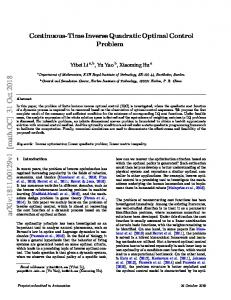
law of the form given in (16), is globally asymptotically stable, then the equilibrium point = 0 (tracking error) for system (40) with control law (37) is globally asymptotically stable for the transformed system along the desired trajectory The minimization of a meaningful cost functional is estab­ lished similarly as in Theorem 2, and hence it is omitted. Fig. 1 displays the proposed transformation and optimality scheme.

(32)

Zk

These steps are taken iteratively. At the last step, the known desired variable is and the last new variable is defined as

xS,k'

Xo, k.

As usually, taking one step ahead yields

Z

r (Xk) + Br (Xk) a( xk) - XS,k+l

(38)

jl (Z!) + Bl (Z!) Z�

Zk1+l

The desired dynamics for this block is imposed as

=

L (l( Zk) + j3T( Zk) R( Zk) j3( Zk)) k=O

Proof The closed-loop dynamics of system (34) and control law (36) results in

=

kZ +l

=

(39)

x� k

j 2 (xLx%) + B 2 (xLx%) x� - X�, k+l jl (Z!) + B 2 (L z D z �z

(37)

with

2 ' Zk2 X2k - xo,k Taking one step ahead in � z yields 2Zk+l 2 2 Xk+l - Xo,k+l j 2 (xLx%) + B 2 (xLx%) x� - X�,k+l' Z�+1

gT( Zk) P j( Zk).

00

J

x�

x%

)-1

Moreover, control law (37) is inverse optimal in the sense that it minimizes the meaningful cost functional:

Note that the calculated value of state kin (31) is not the real value of such state; instead of, it represents the desired behavior for Hence, to avoid confusions this desired value of is referred as in (31). Proceeding in the s�e way as for the first block, a second variable in the new coordinates is defined as

x%.

9(Xk)

p

•

(33) A.

Then, system (27) can be presented in the new variables = of the form

[ Z IT z 2T ... z rTJ !z +l jl (Z!) + Bl (Z!) z�

Example

In this section, we illustrate the applicability of the obtained results by means of an unstable example for solving the trajectory tracking problem. By illustration easily and space limitation, we synthesize an trajectory tracking inverse optimal control law for a discrete-time second order system (unstable for = 0) of the form (1) with:

Uk

(34)

j(Xk)

5

=

[

Xl, k + X2,k Xl, k + 2X2,k

1 .5

(41)

Block Control Form System

Xk+l

=

ACKNOWLEDGMENT

The authors thanks to CONACyT, Mexico, for support on projects 131678 and 46069.

!(Xk) + g(xk) a(xk)

�

REFERENCES

Control Law

a(xk)

[1] R. Sepulchre, M. Jankovic, and P. V Kokotovic, Constructive Nonlinear Control. London, New York, USA: Springer-Verlag, 1997. [2] M. Krstic and H. Deng, Stabilization of Nonlinear Uncertain Systems. Secaucus, NJ, USA: Springer-Verlag New York, Inc., 1998. [3] B. D. O. Anderson and J. B. Moore, Optimal Control: Linear Quadratic Methods. Englewood Cliffs, New Jersey, USA: Prentice-Hall, 1990. [4] R. E. Kalman, "When is a linear control system optimal?" Transactions of the ASM E, lournal of Basic Engineering, Series D, vol. 86, pp. 81-90, 1964. [5] R. A. Freeman and P. V Kokotovic, "Optimal nonlinear controllers for feedback linearizable systems," in Proceedings of the 14th American Control Coriference, 1995, vol. 4, Seattle, WA, USA, June 1995, pp. 2722-2726. [6] P. J. Moylan and B. D. O. Anderson, "Nonlinear regulator theory and an inverse optimal control problem," IEEE Transactions on Automatic Control, vol. 18, no. 5, pp. 460-465, 1973. [7] J. L. Willems and H. V D. Voorde, "Inverse optimal control problem for linear discrete-time systems," Electronics Letters, vol. 13, p. 493, Aug 1977. [8] L. Magni and R. Sepulchre, "Stability margins of nonlinear receding horizon control via inverse optimality," Systems and Control Letters, vol. 32, no. 4, pp. 241-245, 1997. [Online]. Available: http://www.montefiore.ulg.ac.be/services/stochastic/pubsl19971MS97 [9] R. A. Freeman and P. V Kokotovic, Robust nonlinear control de­ sign: state-space and Lyapunov techniques. Cambridge, MA, USA: Birkhauser Boston Inc., 1996. [10] T. Ahmed-Ali, F. Mazenc, and F. Lamnabhi-Lagarrigue, "Disturbance attenuation for discrete-time feedforward nonlinear systems," Lecture notes in control and iriformation sciences, vol. 246, pp. 1-17, March 1999. [II] F. Ornelas, E. N. Sanchez, and A. G. Loukianov, "Discrete-time inverse optimal control for nonlinear systems trajectory tracking," in Proceed­ ings of the 49th IEEE Conference on Decision and Control, Atlanta, Georgia, USA, Dec 2010, pp. 4813-4818. [12] R. A. Freeman and P. V Kokotovic, "Inverse optimality in robust stabilization," SIAM lournal on Control and Optimization, vol. 34, no. 4, pp. 1365-1391, 1996. [13] J. A. Primbs, V Nevistic, and J. C. Doyle, "Nonlinear optimal control: A control Lyapunov function and receding horizon perspective," Asian lournal of Control, vol. I, pp. 14-24, 1999. [14] R. A. Freeman and 1. A. Primbs, "Control Lyapunov functions: New ideas from an old source," in Proceedings of the 35th IEEE Conference on Decision and Control, Kobe, Japan, 1996, pp. 3926-3931. [15] D. E. Kirk, Optimal Control Theory: An Introduction. Prentice-Hall, NJ, USA, 1970. [16] F. L. Lewis and V L. Syrmos, Optimal control. John Wiley & Sons, New York, USA, 1995. [17] T. Basar and G. J. Olsder, Dynamic noncooperative game theory, 2nd ed. Academic Press, New York, 1995. [18] A. Al-Tamimi and F. L. Lewis, "Discrete-time nonlinear HJB solution using approximate dynamic programming: Convergence proof," IEEE Transactions on Systems, Man, Cybernetics-Part B, vol. 38, no. 4, pp. 943-949, August 2008. [19] T. Ohsawa, A. M. Bloch, and M. Leok, "Discrete Hamilton-Jacobi theory," 2009. [Online]. Available: http://www.citebase.org/abstract?id= oai:arXiv.org:09I1.2258 [20] W. M. Haddad, V-So Chellaboina, J. L. Fausz, and C. Abdallah, "Optimal discrete-time control for non-linear cascade systems," lournal of The Franklin Institute, vol. 335, no. 5, pp. 827-839, 1998. [21] H. K. Khalil, Nonlinear Systems. New Jersey: Prentice Hall, 1996. [22] G. L. Amicucci, S. Monaco, and D. Normand-Cyrot, "Control Lyapunov stabilization of affine discrete-time systems," vol. I, San Diego, CA, USA, Dec. 1997, pp. 923-924. [23] M. Vidyasagar, Nonlinear systems analysis, 2nd ed. Prentice Hall, 1993. [24] A. G. Loukianov, "Nonlinear block control with sliding modes," Au­ tomation and Remote Control, vol. 57, no. 7, pp. 916-933, 1998.

(XS,k+1 - !(xk) + !(Zk) + B(Zk) !3(Zk) B(xk)

=

-I

�

Transformed System

Zk+l

=

!(Zk) + g(Zk) /3(Zk)

�

Meaningful Cost Functional 00

:J

=

2)I(zk) + (3T(Zk) R(Zk) (3(Zk» k�O

Fig. 1. Transformation scheme and inverse optimal control for transformed system.

0

��

20

40

:1 •

-20

20

40

Time(k)

Time(k)

60

80

•

60

80

100

•

100

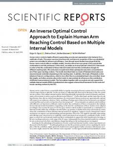
Fig. 2. Tracking performance of Xk. Solid line (X8,k) is the reference signal and dashed line is the evolution of XI,k. Control signal is also displayed.

and

(42) In accordance with Section IV , control law (36) becomes

X�,k+2 +5.25

with

for

a( z k)' Fig.

Xl, k 1 .5 X2,k Zl, k + 3.5 Z2,k + 2a( z k)'

-

3.25

-

(43)

p= [ 100 100]

2 presents the trajectory tracking for Xl, k. V.

CONCLUSIONS

This paper has presented a discrete-time inverse optimal control, which achieve trajectory tracking and is inverse opti­ mal in the sense that it, a posteriori, minimizes a meaningful cost functional. Simulation results illustrate that the required goal is achieved, i.e., the designed controller maintains stabil­ ity on reference for the system.

6