From Inverse Kinematics to Optimal Control

From Inverse Kinematics to Optimal Control Perle Geoffroy†,∗ , Nicolas Mansard∗ , Maxime Raison† , Sofiane Achiche† , Yuval Tassa4 , and Emo Todorov4

Abstract Numerical optimal control (the approximation of an optimal trajectory using numerical iterative algorithms) is a promising approach to compute the control of complex dynamical systems whose instantaneous linearization is not meaningful. Aside from the problems of computation cost, these methods raise several conceptual problems, like stability, robustness, or simply understanding of the nature of the obtained solution. In this paper, we propose a rewriting of the Differential Dynamic Programing solver. Our variant is more efficient and numerically more interesting. Furthermore, it draws some interesting comparisons with the classical inverse formulation: in particular, we show that inverse kinematics can be seen as singular case of it, when the preview horizon collapses. Key words: optimal control,inverse kinematics, differential dynamic programming

1 Introduction Both inverse geometry [11] and inverse kinematics1 [21] can be viewed as the resolution of an optimization problem: non-linear from the configuration space to the special Euclidean group SE(3) for the first one [3], quadratic in the tangent space to the configuration space for the second [5]. This is only one view of the problem, but it helps to formulate efficient solvers and to understand their convergence properties, by using some powerful results of numerical optimization [14]. For controlling a robot, inverse kinematics is nowadays a standard technique, due to its simplic† Ecole Polytechnique de Montr´eal, Montr´eal, Canada. LAAS-CNRS, Univ. Toulouse, Toulouse, France. 4 Univ. Washington, Seattle, USA. ∗

1

The problem we name inverse geometry is sometimes referred as inverse kinematics, the second being referred as differential (or closed-loop) inverse kinematics. We use ‘geometry’ when only static postures are implied and keep the word ‘kinematics’ when a motion is explicitly implied.

1

2

Perle Geoffroy, Nicolas Mansard et al.

ity and the limited computation cost (e.g. 1ms is enough to invert the kinematics of a 40DOF humanoid robot [5]). Moreover, the structure of the problem is well understood and problems are easy to diagnose. On the other hand, model predictive control (MPC) is an advanced technique to control a given system by optimizing its predicted evolution [1]. It relies on the systematic evaluation of the control of the system with respect to a reference cost function, while only the first few steps of the optimal trajectory are executed before its complete re-evaluation. The main interest of MPC is the ability of dealing with non-linear systems whose instantaneous linearization is not meaningful. Like for inverse kinematics, MPC can be formulated as the resolution at each control cycle of a numerical optimization problem depending on the estimated state. However, the typical size of the problem generally makes it difficult to obtain realtime performance [12]. Moreover, this kind of formulation is difficult to interpret. It is typically difficult to quantify the robustness of such controllers [1], or even to explain the reasons that have led to the chosen trajectory. In this paper, we consider an optimal-control solver named Differential Dynamic Programming [8]. This numerical scheme provides a simple yet efficient solver of direct implicit (shooting) optimal-control problems, that makes it possible to control complex systems, like humanoid robots [18], despite the inherent complexity of this class of problems. We propose a reformulation that provides numerical advantages and, more importantly, gives a better understanding of the structure of the optimal trajectory. In particular, when only the robot kinematics are considered, we show that every iteration of the algorithm amounts to a sequence of Jacobian pseudoinversions along the trajectory. Classical pseudoinverse-based inverse kinematics is then equivalent to the optimization of a single-step trajectory. Consequently, once the ratio between the size of the system and the CPU load are sufficiently low, any inverse-kinematics should be considered with several steps ahead rather than with only a single one. The same observation seems valid for inverse dynamics [9].

2 Model predictive control 2.1 Principles and model Consider generic dynamical system, with state x and control u: xt+1 = f (xt , ut ,t)

(1)

f is the evolution function and the time variable t is discrete. x is typically a finite sequence of derivatives of the configuration q, e.g. x = (q, q). ˙ Optimal control computes the control and state trajectories that minimize a given cost function: T −1

min X,U

∑ lt (xt , ut ) + lT (xT )

t=0

From Inverse Kinematics to Optimal Control

3

subject to the constraint (1), where T is the preview-interval length (fixed here), U = (u0 ...uT −1 ) and X = (x0 , ..., xT ) are the control and state trajectories and lt and lT are the running and terminal cost functions. Linear dynamics and quadratic cost lead to the linear-quadratic regulator, given by Riccati equations. In practice, the information contained in X and U is somehow redundant. The problem is reformulated as a problem only on X or only U (the other variable being deduced from the dynamic equation). The formulation is said explicit when computing X [13] (designated also by collocation [16]) and implicit when computing U [17] (designated also by shooting [10]). Both formulations have pros and cons [2]. We consider in the following the implicit formulation, cheaper to solve in practice, without the drawback that it might involve more local minima. For each formulation, the solution to the numerical problem is then approximated using any optimization solver, typically using Newton or quasi-Newton [6] descent.

2.2 Differential dynamic programming Differential Dynamic Programming (DDP) is an iterative algorithm to solve a nonlinear optimal control problem using implicit formulation [17]. It is nearly equivalent to the application of a Newton descent algorithm [15]. As in the Newton descent, it approaches a local optimum by iteratively modifying a candidate solution. It starts with initial state and control trajectories (e.g. obtained by integration of the zero control) and then iterates in two stages. It first computes a quadratic model of the variation of current candidate trajectory and computes the corresponding linearquadratic regulator (LQR – backward loop). The candidate is then modified following the LQR (forward loop). Quadratic model: We denote vt the cost-to-go function defined by: T −1

vt (Xt ,Ut ) =

∑ lk (xk , uk ) + lT (xT ) k=t

where Xt = (xt ..xT ) and Ut = (ut ..uT −1 ) are the trajectory tails. To simplify, we drop the t variable and denote the next quantity at t + 1 by a prime: v0 ≡ vt+1 . DDP relies on the Bellman principle. It proceeds recursively backward in time using the following equation:
v∗ (X,U) = min l(x, u) + v0∗ (X 0 ,U 0 ) 0 0 x,u,X ,U

building a quadratic model of v from the quadratic models of l and v0∗ : 1 v(x + ∆ x,u + ∆ u) = v(x, u) + vx ∆ x + vu ∆ u + ∆ xT vxx ∆ x + ∆ uT vux ∆ x 2 1 + ∆ uT vuu ∆ u + o(||∆ x||2 + ||∆ u||2 ) 2

4

Perle Geoffroy, Nicolas Mansard et al.

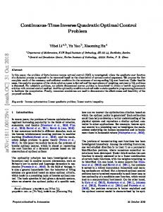
Fig. 1 Snapshots of a whole-body grasping movement on a 25-DOF humanoid robot. The control is computed in real-time. Courtesy from [19].

The quadratic model is defined by the quadratic coefficients vx , vu , vxx , vux and vuu , functions of the derivatives of l, f and v0 (see [17] for details). Backward pass: The optimum ∆ u can be computed for any ∆ x. It is obtained at the zero of the derivative of the quadratic model: ∆ u∗ = λ + Λ ∆ x

(2)

−1 where λ = v−1 uu vx and Λ = vuu vux are the open-loop and close-loop gains. From the optimal change ∆ u∗ , the quadratic model of v∗ can be computed:

v∗x = vx − Λ T vuu λ

(3)

v∗xx = vxx − Λ T vuuΛ

(4)

The backward pass starts from the quadratic model of lT and then recursively computes the optimal gains of all the control cycles from T − 1 down to 0. Forward pass: The forward pass then computes the new candidate trajectory and control schedule. For each control cycle, a new control schedule u˜ is established using (2). For each new u, ˜ the changes is x are obtained by integrating (1) from x0 and then propagated through the closed-loop gains of the next time: ∆ x0 = x0 − f (x, u), ˜

u˜ = u + λ + Λ ∆ x

Performance: The interest of DDP is that its simple formulation can be easily implemented in an efficient way, taking into account the inherent sparsity of a numerical optimal control problem. For example, in [18], a dedicated solver was demonstrated to animate a humanoid virtual avatar in real-time in interaction with a user through a haptic device. It was used to control a simulated 25-DOF HRP2 robot in real-time [19]. In that case, the preview horizon was 0.5s. The preview control was computed in 50ms and then interpolated using the underlying LQR at 5ms, enabling effective real-time control (see Fig. 1).

From Inverse Kinematics to Optimal Control

5

3 Square-root Differential Dynamic Programming In this section we present our proposed modification the the DDP algorithm. The key idea is to propagate the Value Hessian in square-root form. Reminiscent of the square-root Kalman Filter, this formulation ensures positive definiteness and confers numerical stability.

3.1 Algorithm derivation The Gauss-Newton approximation: Very often in practice, both the running and terminal costs have sum-of-square form, with the residuals r(x, u) : l(x, u) = r(x, u)T r(x, u) This specific shape is interesting in practice as it leads to a cheap approximation of the second-order derivatives of l in neglecting the second order derivative of r. This is referred as the Gauss-Newton approximation. lxx = rxT rx ,

lux = ruT rx ,

luu = ruT ru

where rx and ru are respectively the derivatives of r by respect x and u. The approximation converges to the real Hessian when the residuals r converge to 0, which in general ensures a good convergence. On the other hand, the approximated Hessian is always positive, which prevents the algorithm from violently diverging, as happens when the true Hessian is non-positive. Moreover, the particular shape of the approximated Hessian can be taken into account when inverting it, since we have: −1 T lxx lx = rxT rx


−1

rxT = rx+

where rx+ denotes the Moore-Penrose pseudoinverse of rx and can be efficiently computed without explicitly computing the matrix product rxT rx , using for example the SVD or other orthogonal decompositions [7]. In the literature, the Gauss-Newton approximation of the DDP algorithm is referred as the iterative LQR (iLQR) algorithm [20]. In this section, we take advantage of the square shape of the cost and derivatives to propose a more efficient formulation of this algorithm. This shape will also be used to make some correlations with the classical inverse kinematics. Square-root shape of v∗ : In the DDP backward loop, we have to invert the derivatives of v. Being a sum of squares, the cost-to-go v can be expressed as the square T of some vector v∗ = s∗ s∗ . However, DDP does not explicitly compute sx but rather directly propagates the derivatives v∗xx from v0∗ xx . In the following, we formulate the same propagation while keeping the square shape, by searching the vector sˆ∗ and matrix sˆ∗x such that

6

Perle Geoffroy, Nicolas Mansard et al. T

T

v∗xx = sˆ∗x sˆ∗x

v∗x = sˆ∗x sˆ∗ ,

At the beginning of the backward pass, the square shape is trivially given by s(T ) = r(T ) and sx (T ) = rx (T ). During the backward pass, the previous square-root shapes are written s0 and s0x . The derivative v∗xx is given by the recurrence (3), (4). The square shape of (4) is not trivial since it appears as a difference, that we can prove to be positive. We denote by s, sx and su the square root of v, vxx and vuu :       sx ru r s = 0 , sx = ∗0 , su = ∗0 s sx fx sx f u 0

0

0

It is easy to show that v0xx = sxT s0x , v0xu = sxT s0u and v0uu = suT s0u . In that case, the gains are given by the pseudoinverse of su : λ = s+ us,

Λ = s+ u sx

Thanks to the Moore-Penrose conditions, we can reduce sˆ∗ and sˆ∗x to: sˆ∗ = s ,

sˆ∗x = (I − su s+ u )sx

3.2 Advantages and discussion Keeping the square shape of vxx avoids some numerical trouble. In particular, decomposing sx instead of vuu offers much better numerical behavior. Moreover, it avoids the complexity of a big matrix multiplication. This is formalized below. Comparison of the costs: To evaluate the complexity of this algorithm, sizes of x, u and r are supposed all equal to n. The cost for one iteration of the loops is 8n3 , against 11n3 for the classical DDP. Moreover, most operations are due to the QR decompositions and could be performed when computing the derivatives, that leads to a total cost of roughly 3n3 . Pseudo inverse and projection: The gains and propagation closed forms also provide a better understanding of the nature of the inversion. As in the derivation, we consider only the current time of the backward loop. The Jacobian su is the derivative of the cost-to-go. The open-loop gain s+ u s only tries to find the current control that minimizes the cost-to-go evolution. In most of cases, su has more rows than columns. The pseudoinverse will only provide the control that has the maximum efficiency in the least-square sense. What remains is a part of the cost that can be nullified. This is given by the orthogonal part to the image of su , i.e. the kernel of sTu , whose projector can be computed by Pu = I − su s+ u. The backward loop then propagates backward the part of the cost that was not accomplished, and that is selected using the projector. The trajectory optimization then corresponds to a sequence of virtual configurations, each of them being moved to optimize its own cost r and to help the configurations ahead in the trajectory by 0 optimizing their residual cost s∗ .

From Inverse Kinematics to Optimal Control

7

4 Kinematic simulation Three-rotations planar (3R) Robot: Due to a lack of space, we only present some analytical results in simulation with a 3R kinematic model. The dynamic evolution function is reduced to a trivial integration scheme f (x, u) = x + ∆tu, with x = q and u = q. ˙ The robot task is to reach a position pre f with the robot end effector p(q) while minimizing the velocities:   w p (p(q) − pre f ) rt = wu u with w p and wu the weights of the two cost components. In this case, the derivative rx is the robot Jacobian Jq while ru = wu I is a regularization term. At the first step T − 1 of the backward loop, the pseudoinverse is: 

wu I su (T − 1) = w p ∆tJq +

+ =

1 †η J w p ∆t q

u where J † denotes the damped inverse [4] with damping η = wwp ∆t . The last term of the trajectory indeed moves following an inverse-kinematics scheme. The same interpretation can be done on the other samples, with a similar regularization and a task that makes a trade-off between going to the target and helping the next sample in the trajectory to accomplish its residual.

Results: The Square Root algorithm on the simulated 3R Robot was implemented in C++. The control sampling frequency is 1 kHz and the cycle of the robot lasted 0.1s (100 timesteps). We chose wu = 0.01 and w p = 1. The control reaches easily the target with a proper smoothing of the control, as expecting with such a simple system. With this setting, the robot needs 0.1s to reach the target i.e. 100 control cycles. We mainly focus the discussion on the comparison with inverse kinematics. As explained above, inverse kinematics is obtained when the horizon T is reduced to 1. On the opposite extreme, the optimum of the infinite-horizon problem is approximately obtained for a preview horizon of 0.1s (which is the time to the goal). We consider the performance in both the obtained cost and the computation load for T varying from 1 to 100. A summary of the results is given by Fig. 2. On the left figure, we consider the total cost for the overall executed trajectory. This cost is computed a posteriori, after the execution by the robot. The cost is minimal when T is maximal and vice-versa. Most of the cost increase when T is small is due to the increase of the control term (with an artificial apparent minimum for some T = 10 that is due to the ratio over a changing total quantity). On the other hand, the computation load (right figure) increases linearly with the horizon length (as expected). After a certain threshold on the horizon length, the obtained trajectories are the same, with same costs. As always with MPC, the horizon length has to be carefully adjusted: not to small, to find the best trajectory and not to big to limit computation times.

8

Perle Geoffroy, Nicolas Mansard et al. 8

2

Cost (%)

1.5

1

0.5

7 Computation Time (%)

Total Cost Control Cost

6 5 4 3 2 Computation Time

1

0

0

20

40 60 Preview Horizon Length

80

100

0

0

20

40 60 Preview Horizon Length

80

100

Fig. 2 Performance and computation ratio with respect to the preview length. (left) Evolution of the cost when increasing the preview horizon: the total cost is plotted as a ratio with respect to the infinite-horizon optimum. Indicatively, the percentage of the control term of the cost (integral of the velocity norm) is also given. (right) Computation load, plotted as a ratio of the load needed to compute the trajectory with a single-step horizon (i.e. cost of an inverse kinematics). The cost increases linearly with the size of the horizon.

Inverse kinematics is obtained for T = 1. The cost is the lowest, but a poor resulting cost. For only a small expense, (e.g. T = 4), better trajectories are obtained.

5 Conclusion In this paper, we described a square-root formulation of the DDP algorithm. The formulation is numerically more efficient, improving both the computation load and the numerical conditioning. It also makes apparent the relation between MPC and other optimization-based robot algorithms. In particular, it makes use of a sequence of pseudo-inverses of the cost Jacobian along the trajectory. In the particular case where the time evolution function is reduced to the robot kinematics, this sequence is equal to the pseudo-inverse of the cost Jacobian, with the first term of the trajectory following exactly an inverse-kinematics scheme for the final cost. This study reveals that inverse kinematics is nothing but an MPC scheme with a singular horizon, and that the robot behavior might be very much improved by simply considering a few samples ahead of the current robot position when computing an inverse-kinematics scheme. The same principle should apply with more complex time-evolution function. For example, when considering the robot dynamics (the state being the configuration and velocity, and the control being joint torques), MPC should meet the operationalspace inverse dynamics when the preview horizon collapses.

From Inverse Kinematics to Optimal Control

9

References 1. Alamir, M.: Stabilization of Nonlinear Systems Using Receding-Horizon Control Schemes. Lecture Notes in Control and Information Sciences. Springer (2006) 2. Biegler, L.: Nonlinear programming: concepts, algorithms, and applications to chemical processes. SIAM (2010) 3. Das, H., Slotine, J.J., Sheridan, T.: Inverse kinematic algorithms for redundant systems. In: IEEE Int. Conf. on Robotics and Automation (ICRA’88), pp. 43–48. Philadelphia, USA (1988) 4. Deo, A., Walker, I.: Robot subtask performance with singularity robustness using optimal damped least squares. In: IEEE ICRA, pp. 434–441. Nice, France (1992) 5. Escande, A., Mansard, N., Wieber, P.B.: Hierarchical quadratic programming. Int. Journal of Robotics Research (2012). [in press] 6. Goldfarb, D.: A family of variable-metric methods derived by variational means. Mathematics of computation 24(109), 23–26 (1970) 7. Golub, G., Van Loan, C.: Matrix computations, 3rd edn. John Hopkins University Press (1996) 8. Jacobson, D.H., Mayne, D.Q.: Differential Dynamic Programming. Elsevier (1970) 9. Khatib, O.: A unified approach for motion and force control of robot manipulators: The operational space formulation. International Journal of Robotics Research 3(1), 43–53 (1987) 10. Leineweber, D.B., Sch¨afer, A., Bock, H.G., Schl¨oder, J.P.: An efficient multiple shooting based reduced sqp strategy for large-scale dynamic process optimization: Part ii: Software aspects and applications. Computers & chemical engineering 27(2), 167–174 (2003) 11. McCarthy, J.: Introduction to Theoretical Kinematics. MIT Press (1990) 12. Mombaur, K.: Using optimization to create self-stable human-like running. Robotica 27(03), 321 (2008). DOI 10.1017/S0263574708004724 13. Mordatch, I., Todorov, E., Popovi´c, Z.: Discovery of complex behaviors through contactinvariant optimization. In: ACM SIGGRAPH’12. Los Angeles, USA (2012) 14. Nocedal, J., Wright, S.J.: Numerical Optimization, 2nd edn. Springer, New York (2006) 15. Pantoja, D.O.: Differential dynamic programming and newton’s method. International Journal of Control 47(5), 1539–1553 (1988). DOI 10.1080/00207178808906114. URL http://www.tandfonline.com/doi/abs/10.1080/00207178808906114 16. Schulman, J., Lee, A., Awwal, I., Bradlow, H., Abbeel, P.: Finding locally optimal, collisionfree trajectories with sequential convex optimization. Robotics: Science and Systems (2013) 17. Tassa, Y., Erez, T., Todorov, E.: Synthesis and stabilization of complex behaviors through online trajectory optimization. In: (IROS’12). Portugal 18. Tassa, Y., Erez, T., Todorov, E.: Synthesis and stabilization of complex behaviors through online trajectory optimization. In: IEEE/RSJ International Conference on Intelligent Robots and Systems (IROS’12), pp. 4906–4913 (2012). DOI 10.1109/IROS.2012.6386025 19. Tassa, Y., Mansard, N., Todorov, E.: Control-limited differential dynamic programming. Under Review 20. Todorov, E., Li, W.: A generalized iterative LQG method for locally-optimal feedback control of constrained nonlinear stochastic systems. In: Proceedings of the American Control Conference (ACC’05), pp. 300–306. Portland, OR, USA (2005). DOI 10.1109/ACC.2005.1469949 21. Whitney, D.: Resolved motion rate control of manipulators and human prostheses. IEEE Transactions on Man-Machine Systems 10(2), 47–53 (1969)