from control theory is presented, from which the solutions of output estimation, ... The discrete-time system operates on the input signal wk â Rm ...... [15] K. Ogata, Discrete-time Control Systems, Prentice-Hall, Inc., Englewood Cliffs, New.
Discrete-Time Minimum-Variance Prediction and Filtering
75
4 Discrete-Time Minimum-Variance Prediction and Filtering 4.1 Introduction Kalman filters are employed wherever it is desired to recover data from the noise in an optimal way, such as satellite orbit estimation, aircraft guidance, radar, communication systems, navigation, medical diagnosis and finance. Continuous-time problems that possess differential equations may be easier to describe in a state-space framework, however, the filters have higher implementation costs because an additional integration step and higher sampling rates are required. Conversely, although discrete-time state-space models may be less intuitive, the ensuing filter difference equations can be realised immediately. The discrete-time Kalman filter calculates predicted states via the linear recursion xˆ k 1/ k Ak xˆ k 1/ k K k ( zk C k xˆ k 1/ k ) ,
where the predictor gain, Kk, is a function of the noise statistics and the model parameters. The above formula was reported by Rudolf E. Kalman in the 1960s [1], [2]. He has since received many awards and prizes, including the National Medal of Science, which was presented to him by President Barack Obama in 2009. The Kalman filter calculations are simple and well-established. A possibly troublesome obstacle is expressing problems at hand within a state-space framework. This chapter derives the main discrete-time results to provide familiarity with state-space techniques and filter application. The continuous-time and discrete-time minimum-square-error Wiener filters were derived using a completing-the-square approach in Chapters 1 and 2, respectively. Similarly for time-varying continuous-time signal models, the derivation of the minimum-variance Kalman filter, presented in Chapter 3, relied on a least-mean-square (or conditional-mean) formula. This formula is used again in the solution of the discrete-time prediction and filtering problems. Predictions can be used when the measurements are irregularly spaced or missing at the cost of increased mean-square-error. This chapter develops the prediction and filtering results for the case where the problem is nonstationary or time-varying. It is routinely assumed that the process and measurement noises are zero mean and uncorrelated. Nonzero mean cases can be accommodated by including deterministic inputs within the state prediction and filter output updates. Correlated noises can be handled by adding a term within the predictor gain and the underlying Riccati equation. The same approach is employed when the signal model “Man will occasionally stumble over the truth, but most of the time he will pick himself up and continue on.” Winston Leonard Spencer-Churchill
Smoothing, Filtering and Prediction: Estimating the Past, Present and Future
76
possesses a direct-feedthrough term. A simplification of the generalised regulator problem from control theory is presented, from which the solutions of output estimation, input estimation (or equalisation), state estimation and mixed filtering problems follow immediately. wk
∑
Bk
xk+1
z-1
xk
Ck
∑
yk
Ak Dk
Figure 1. The discrete-time system operates on the input signal wk m and produces the output yk p . 4.2 The Time-varying Signal Model A discrete-time time-varying system : m → p is assumed to have the state-space representation x k 1 Ak xk Bk wk ,
(1)
y k C k x k Dk wk ,
(2)
where Ak n n , Bk n m , Ck p n and Dk p p over a finite interval k [0, N]. The wk is a stochastic white process with E{wk } = 0, E{w j wTk } = Qk jk ,
(3)
1 if j k in which jk is the Kronecker delta function. This system is depicted in Fig. 1, 0 if j k in which z-1 is the unit delay operator. It is interesting to note that, at time k the current state
xk = Ak-1xk-1 + Bk-1wk-1,
(4)
does not involve wk. That is, unlike continuous-time systems, here there is a one-step delay between the input and output sequences. The simpler case of Dk = 0, namely,
yk = Ckxk,
(5)
is again considered prior to the inclusion of a nonzero Dk.
“Rudy Kalman applied the state-space model to the filtering problem, basically the same problem discussed by Wiener. The results were astonishing. The solution was recursive, and the fact that the estimates could use only the past of the observations posed no difficulties.” Jan. C. Willems
Discrete-Time Minimum-Variance Prediction and Filtering
77
4.3 The State Prediction Problem Suppose that observations of (5) are available, that is,
zk = yk + vk,
(6)
where vk is a white measurement noise process with
E{vk} = 0, E{v j vTk } = Rkδjk and E{w j vTk } =0.
wk
vk
yk
(7)
zk
∑
yˆ k / k 1
∑
ek / k 1 y k yˆ k / k 1
Figure 2. The state prediction problem. The objective is to design a predictor which operates on the measurements and produces state estimates such that the variance of the error residual ek/k-1 is minimised. It is noted above for the state recursion (4), there is a one-step delay between the current state and the input process. Similarly, it is expected that there will be one-step delay between the current state estimate and the input measurement. Consequently, it is customary to denote xˆ k / k 1 as the state estimate at time k, given measurements at time k – 1. The xˆ k / k 1 is also known as the one-step-ahead state prediction. The objective here is to design a predictor that operates on the measurements zk and produces an estimate, yˆ k / k 1 = C k xˆ k / k 1 , of yk = Ckyk, so that the covariance, E{ek / k 1eTk / k 1} , of the error residual, ek/k-1 = yk – yˆ k / k 1 , is minimised. This problem is depicted in Fig. 2 4.4 The Discrete-time Conditional Mean Estimate The predictor derivation that follows relies on the discrete-time version of the conditionalmean or least-mean-square estimate derived in Chapter 3, which is set out as follows. Consider a stochastic vector [ kT
T
kT ] having means and covariances E k k
“Prediction is very difficult, especially if it’s about the future.” Niels Henrik David Bohr
(8)
Smoothing, Filtering and Prediction: Estimating the Past, Present and Future
78
and E k kT k
k k
k k
kT
k k . k k
(9)
respectively, where k k T k k . An estimate of k given k , denoted by E{ k | k } , which
minimises E( k − E{ k | k })( k − E{ k | k })T , is given by E{ k | k } k k 1k k ( k ) .
(10)
The above formula is developed in [3] and established for Gaussian distributions in [4]. A derivation is requested in the problems. If αk and βk are scalars then (10) degenerates to the linear regression formula as is demonstrated below. Example 1 (Linear regression [5]). The least-squares estimate ˆ k = a k + b of k given data
αk, βk over [1, N], can be found by minimising the performance objective J =
ˆ ) 2 =
1 N
N
( k 1
k
– a k – b) 2 . Setting
1 N
N
( k 1
k
–
dJ dJ = 0 yields b = a . Setting = 0, substituting da db
for b and using the definitions (8) – (9), results in a = k k 1k k . 4.5 Minimum-Variance Prediction It follows from (1), (6), together with the assumptions E{wk} = 0, E{vk} = 0, that E{xk+1} = E{Akxk} and E{zk} = E{Ckxk}. It is assumed that similar results hold in the case of predicted state estimates, that is, xˆ A xˆ E k 1 k k / k 1 . ˆ z C x k k k / k 1
(11)
Substituting (11) into (10) and denoting xˆ k 1/ k = E{xˆ k 1 | zk } yields the predicted state xˆ k 1/ k Ak xˆ k / k 1 K k ( zk C k xˆ k / k 1 ) ,
where Kk
(12)
E{xˆ k 1zTk }E{zk zTk }1 is known as the predictor gain, which is designed in the next
section. Thus, the optimal one-step-ahead predictor follows immediately from the leastmean-square (or conditional mean) formula. A more detailed derivation appears in [4]. The structure of the optimal predictor is shown in Fig. 3. It can be seen from the figure that produces estimates yˆ k / k 1 = C k xˆ k / k 1 from the measurements zk.
“I admired Bohr very much. We had long talks together, long talks in which Bohr did practically all the talking.” Paul Adrien Maurice Dirac
Discrete-Time Minimum-Variance Prediction and Filtering
zk
zk Ck xˆ k / k 1 Σ
Kk
─
79
xˆ k 1/ k
z-1
Σ
yˆ k / k 1 Ck xˆ k / k 1
Ak
Ck xˆ k / k 1
Figure 3. The optimal one-step-ahead predictor which produces estimates xˆ k 1/ k of xk+1 given measurements zk. Let x k / k 1 = xk – xˆ k / k 1 denote the state prediction error. It is shown below that the expectation of the prediction error is zero, that is, the predicted state estimate is unbiased. Lemma 1: Suppose that xˆ 0 / 0 = x0, then E{x k 1/ k } = 0
(13)
for all k [0, N]. Proof: The condition xˆ 0 / 0 = x0 is equivalent to x 0 / 0 = 0, which is the initialisation step for an induction argument. Subtracting (12) from (1) gives x k 1/ k ( Ak K kC k )x k / k 1 Bk wk K k vk
(14)
E{x k 1/ k } ( Ak K kC k )E{x k / k 1} Bk E{wk } K k E{vk } .
(15)
and therefore
From assumptions (3) and (7), the last two terms of the right-hand-side of (15) are zero. Thus, (13) follows by induction. � 4.6 Design of the Predictor Gain It is shown below that the optimum predictor gain is that which minimises the prediction error covariance E{x k / k 1x Tk / k 1} . Lemma 2: In respect of the estimation problem defined by (1), (3), (5) - (7), suppose there exist solutions Pk / k 1 = PkT/ k 1 ≥ 0 to the Riccati difference equation Pk 1/ k Ak Pk / k 1 ATk BkQk BTk Ak Pk / k 1C Tk (C k Pk / k 1C Tk Rk ) 1C k Pk / k 1 ATk ,
(16)
over [0, N], then the predictor gain K k Ak Pk / k 1C Tk (C k Pk / k 1C Tk Rk ) 1 ,
(17)
within (12) minimises Pk / k 1 = E{x k / k 1x Tk / k 1} .
“When it comes to the future, there are three kinds of people: those who let it happen, those who make it happen, and those who wondered what happened.” John M. Richardson Jr.
Smoothing, Filtering and Prediction: Estimating the Past, Present and Future
80
Proof: Constructing Pk 1/ k E{x k 1/ k x Tk 1 / k } using (3), (7), (14), E{x k / k 1wTk } = 0 and E{x k / k 1vTk } = 0 yields Pk 1/ k ( Ak K k Ck ) Pk / k 1 ( Ak K k Ck )T Bk Qk BkT K k Rk K kT ,
(18)
which can be rearranged to give Pk 1/ k Ak Pk / k 1 ATk Ak Pk / k 1C Tk (C k Pk / k 1C Tk Rk ) 1C k Pk / k 1 ATk BkQk BTk (K k Ak Pk / k 1C Tk (C k Pk / k 1C Tk Rk ) 1 )(C k Pk / k 1C Tk Rk )
(19)
(K k Ak Pk / k 1C Tk (C k Pk / k 1C Tk Rk ) 1 )T ,
By inspection of (19), the predictor gain (17) minimises Pk 1/ k .
�
4.7 Minimum-Variance Filtering It can be seen from (12) that the predicted state estimate xˆ k / k 1 is calculated using the previous measurement zk-1 as opposed to the current data zk. A state estimate, given the data at time k, which is known as the filtered state, can similarly be obtained using the linear least squares or conditional-mean formula. In Lemma 1 it was shown that the predicted state estimate is unbiased. Therefore, it is assumed that the expected value of the filtered state equals the expected value of the predicted state, namely, xˆ xˆ E k / k k / k 1 . ˆ z C x k k k / k 1
(20)
Substituting (20) into (10) and denoting xˆ k / k = E{xˆ k | zk } yields the filtered estimate xˆ k / k xˆ k / k 1 Lk ( zk C k xˆ k / k 1 ) ,
(21)
where Lk = E{xˆ k zTk }E{zk zTk }1 is known as the filter gain, which is designed subsequently. Let x k / k = xk – xˆ k / k denote the filtered state error. It is shown below that the expectation of the
filtered error is zero, that is, the filtered state estimate is unbiased. Lemma 3: Suppose that xˆ 0 / 0 = x0, then E{x k / k } = 0
(22)
for all k [0, N].
“To be creative you have to contribute something different from what you've done before. Your results need not be original to the world; few results truly meet that criterion. In fact, most results are built on the work of others.” Lynne C. Levesque
Discrete-Time Minimum-Variance Prediction and Filtering
81
Proof: Following the approach of [6], combining (4) - (6) results in zk = CkAk-1xk-1 + CkBk-1wk-1 + vk, which together with (21) yields x k / k ( I LkC k ) Ak 1x k 1/ k 1 ( I LkC k )Bk 1wk 1 Lk vk . (23)
From (23) and the assumptions (3), (7), it follows that E{x k / k } ( I LkC k ) Ak 1E{x k 1/ k 1}
( I LkC k ) Ak 1 ( I L1C1 ) A0E{x 0 / 0 } .
Hence, with the initial condition xˆ 0 / 0 = x0, E{x k / k } = 0.
(24) �
4.8 Design of the Filter Gain It is shown below that the optimum filter gain is that which minimises the covariance E{x k / k x Tk / k } , where x k / k = xk – xˆ k / k is the filter error. Lemma 4: In respect of the estimation problem defined by (1), (3), (5) - (7), suppose there exists a solution Pk / k = PkT/ k ≥ 0 to the Riccati difference equation Pk / k Pk / k 1 Pk / k 1C Tk (C k Pk / k 1C Tk Rk ) 1C k Pk / k 1 ,
(25)
over [0, N], then the filter gain Lk Pk / k 1C Tk (C k Pk / k 1C Tk Rk ) 1 ,
(26)
within (21) minimises Pk / k E{x k / k x Tk / k } . Proof: Subtracting xˆ k / k from xk yields x k / k = xk – xˆ k / k = xk − xˆ k / k 1 − Lk (Cx k + vk − Cxˆ k / k 1 ) , that is, x k / k ( I LkC k ) x k / k 1 Lk vk
(27)
Pk / k ( I LkC k ) Pk / k 1 ( I LkC k )T Lk Rk LTk ,
(28)
and which can be rearranged as7 Pk / k Pk / k 1 Pk / k 1C Tk (C k Pk / k 1C Tk Rk ) 1C k Pk / k 1 (Lk Pk / k 1C Tk (C k Pk / k 1C Tk Rk ) 1 )(C k Pk / k 1C Tk Rk )(Lk Pk / k 1C Tk (C k Pk / k 1C Tk Rk ) 1 )T
By inspection of (29), the filter gain (26) minimises Pk / k .
(29) �
Example 2 (Data Fusion). Consider a filtering problem in which there are two measurements of 1 the same state variable (possibly from different sensors), namely Ak, Bk, Qk , Ck = and Rk 1 0 R1, k = , with R1,k, R2,k . Let Pk/k-1 denote the solution of the Riccati difference equation 0 R 2, k (25). By applying Cramer’s rule within (26) it can be found that the filter gain is given by “A professor is one who can speak on any subject - for precisely fifty minutes.” Norbert Wiener
Smoothing, Filtering and Prediction: Estimating the Past, Present and Future
82
R2, k Pk / k 1 Lk R P 2, k k / k 1 R1, k Pk / k 1 R1, k R2, k
from which it follows that
lim
R1, k 0 R2, k 0
R1, k Pk / k 1 , R2, k Pk / k 1 R1, k Pk / k 1 R1, k R2, k
Lk 1 0 and
lim
R2 , k 0 R1, k 0
Lk 0 1 . That is, when the
first measurement is noise free, the filter ignores the second measurement and vice versa. Thus, the Kalman filter weights the data according to the prevailing measurement qualities. 4.9 The Predictor-Corrector Form The Kalman filter may be written in the following predictor-corrector form. The corrected (or filtered) error covariances and states are respectively given by Pk / k Pk / k 1 Pk / k 1C kT (C k Pk / k 1C kT Rk ) 1C k Pk / k 1 T k
(30)
1 T k k
Pk / k 1 Lk (C k Pk / k 1C R ) L ( I LkC k ) Pk / k 1 ,
xˆ k / k xˆ k / k 1 Lk ( zk C k xˆ k / k 1 ) ( I LkC k )xˆ k / k 1 Lk zk ,
(31)
where Lk = Pk / k 1C Tk (C k Pk / k 1C Tk + Rk)-1. Equation (31) is also known as the measurement update. The predicted state and error covariances are respectively given by xˆ k 1/ k Ak xˆ k / k
(32)
( Ak K kC k ) xˆ k / k 1 K k zk , Pk 1/ k Ak Pk / k AkT BkQk BTk ,
(33)
where Kk = Ak Pk / k 1C Tk (C k Pk / k 1C kT + Rk)-1. It can be seen from (31) that the corrected estimate, xˆ k / k , is obtained using measurements up to time k. This contrasts with the prediction at time
k + 1 in (32), which is based on all previous measurements. The output estimate is given by yˆ k / k C k xˆ k / k C k xˆ k / k 1 C k Lk ( zk C k xˆ k / k 1 )
(34)
C k ( I LkC k )xˆ k / k 1 C k Lk zk .
“Before the advent of the Kalman filter, most mathematical work was based on Norbert Wiener's ideas, but the 'Wiener filtering' had proved difficult to apply. Kalman's approach, based on the use of state space techniques and a recursive least-squares algorithm, opened up many new theoretical and practical possibilities. The impact of Kalman filtering on all areas of applied mathematics, engineering, and sciences has been tremendous.” Eduardo Daniel Sontag
Discrete-Time Minimum-Variance Prediction and Filtering
83
4.10 The A Posteriori Filter The above predictor-corrector form is used in the construction of extended Kalman filters for nonlinear estimation problems (see Chapter 10). When state predictions are not explicitly required, the following one-line recursion for the filtered state can be employed. Substituting xˆ k / k 1 = Ak 1xˆ k 1/ k 1 into xˆ k / k = ( I LkC k )xˆ k / k 1 + Lkzk yields xˆ k / k = (I – LkC k ) Ak 1xˆ k 1/ k 1 + Lkzk. Hence, the output estimator may be written as
xˆ k / k ( I LkC k ) Ak 1 Lk xˆ k 1/ k 1 ˆ , Ck zk yk / k
(35)
This form is called the a posteriori filter within [7], [8] and [9]. The absence of a direct feedthrough matrix above reduces the complexity of the robust filter designs described in [7], [8] and [9]. 4.11 The Information Form Algebraically equivalent recursions of the Kalman filter can be obtained by propagating a so-called corrected information state xˆ k / k Pk/1k xˆ k / k ,
(36)
xˆ k 1/ k Pk11/ k xˆ k 1/ k .
(37)
( A BCD) 1 A1 A1B(C 1 DA1B) 1 DA1 ,
(38)
and a predicted information state
The expression
which is variously known as the Matrix Inversion Lemma, the Sherman-Morrison formula and Woodbury’s identity, is used to derive the information filter, see [3], [4], [11], [14] and [15]. To confirm the above identity, premultiply both sides of (38) by ( A BD1C ) to obtain I I BCDA1 B(C 1 DA1B) 1 DA1 BCDA1B(C 1 DA1B) 1 DA1 I BCDA 1 B( I CDA1B) 1 (C 1 DA 1B) 1 DA1 I BCDA1 BC (C 1 DA1B) 1 (C 1 DA 1B) 1 DA1 ,
“I have been aware from the outset that the deep analysis of something which is now called Kalman filtering was of major importance. But even with this immodesty I did not quite anticipate all the reactions to this work.” Rudolf Emil Kalman
Smoothing, Filtering and Prediction: Estimating the Past, Present and Future
84
from which the result follows. From the above Matrix Inversion Lemma and (30) it follows that Pk/1k ( Pk / k 1 Pk / k 1C Tk (C k Pk / k 1C Tk Rk ) 1C k Pk / k 1 ) 1 Pk/1k 1 C Tk Rk1C k ,
(39)
assuming that Pk/1k 1 and Rk1 exist. An expression for Pk11/ k can be obtained from the Matrix Inversion Lemma and (33), namely, Pk11/ k ( Ak Pk / k AkT BkQk BkT ) 1 (Fk1 BkQk BkT ) 1 ,
(40)
where Fk = ( Ak Pk / k ATk ) 1 = AkT Pk/1k Ak1 , which gives Pk11/ k ( I Fk Bk (BkT Fk Bk Qk1 ) 1 BTk )Fk .
(41)
Another useful identity is ( A BCD) 1 BC A1 ( I BCDA1 ) 1 BC A1B( I CDA1B) 1C
(42)
A1B(C 1 DA1B) 1 .
From (42) and (39), the filter gain can be expressed as Lk Pk / k 1C Tk (C k Pk / k 1C Tk Rk ) 1 ( Pk/1k 1 C kT Rk1C k ) 1C kT Rk1
(43)
Pk / kC Tk Rk1 .
Premultiplying (39) by Pk / k and rearranging gives I LkC k Pk / k Pk/1k 1 .
(44)
It follows from (31), (36) and (44) that the corrected information state is given by xˆ k / k Pk/1k xˆ k / k Pk/1k ( I LkC k )xˆ k / k 1 Pk/1k Lk zk
(45)
xˆ k / k 1 C Tk Rk1zk .
“Information is the oxygen of the modern age. It seeps through the walls topped by barbed wire, it wafts across the electrified borders.” Ronald Wilson Reagan
Discrete-Time Minimum-Variance Prediction and Filtering
85
The predicted information state follows from (37), (41) and the definition of Fk, namely, xˆ k 1/ k Pk11/ k xˆ k 1/ k Pk11/ k Ak xˆ k / k ( I Fk Bk (BTk Fk Bk Qk1 ) 1 BTk )Fk Ak xˆ k / k
(46)
( I Fk Bk (BkT Fk Bk Qk1 ) 1 BTk ) AkT xˆ k / k .
Recall from Lemma 1 and Lemma 3 that E{x k xˆ k 1/ k } = 0 and E{x k xˆ k / k } = 0, provided
xˆ 0 / 0 = x0. Similarly, with xˆ 0 / 0 = P0/10 x0 , it follows that E{x k Pk 1/ k xˆ k 1/ k } = 0 and
E{x k Pk / k xˆ k / k } = 0. That is, the information states (scaled by the appropriate covariances) will be unbiased, provided that the filter is suitably initialised. The calculation cost and potential for numerical instability can influence decisions on whether to implement the predictor-corrector form (30) - (33) or the information form (39) - (46) of the Kalman filter. The filters have similar complexity, both require a p × p matrix inverse in the measurement updates (31) and (45). However, inverting the measurement covariance matrix for the information filter may be troublesome when the measurement noise is negligible. 4.12 Comparison with Recursive Least Squares The recursive least squares (RLS) algorithm is equivalent to the Kalman filter designed with the simplifications Ak = I and Bk = 0; see the derivations within [10], [11]. For convenience, consider a more general RLS algorithm that retains the correct Ak but relies on the simplifying assumption Bk = 0. Under these conditions, denote the RLS algorithm’s predictor gain by K k Ak Pk / k 1C kT (C k Pk / k 1C Tk Rk ) 1 ,
(47)
where Pk / k 1 is obtained from the Riccati difference equation Pk 1/ k Ak Pk / k 1 ATk Ak Pk / k 1C Tk (C k Pk / k 1C Tk Rk ) 1C k Pk / k 1 ATk .
(48)
It is argued below that the cost of the above model simplification is an increase in meansquare-error. Lemma 5: Let Pk 1/ k denote the predicted error covariance within (33) for the optimal filter. Under
the above conditions, the predicted error covariance, Pk / k 1 , exhibited by the RLS algorithm satisfies Pk / k 1 Pk / k 1 .
(49)
“All of the books in the world contain no more information than is broadcast as video in a single large American city in a single year. Not all bits have equal value.” Carl Edward Sagan
Smoothing, Filtering and Prediction: Estimating the Past, Present and Future
86
Proof: From the approach of Lemma 2, the RLS algorithm’s predicted error covariance is given by Pk 1/ k Ak Pk / k 1 ATk Ak Pk / k 1C Tk (C k Pk / k 1C Tk Rk ) 1C k Pk / k 1 ATk BkQk BTk (K k Ak Pk / k 1C kT (C k Pk / k 1C kT Rk ) 1 )(C k Pk / k 1C Tk Rk )
(50)
(K k Ak Pk / k 1C Tk (C k Pk / k 1C Tk Rk ) 1 )T .
The last term on the right-hand-side of (50) is nonzero since the above RLS algorithm relies on the � erroneous assumption BkQk BkT = 0. Therefore (49) follows. 4.13 Repeated Predictions When there are gaps in the data record, or the data is irregularly spaced, state predictions can be calculated an arbitrary number of steps ahead. The one-step-ahead prediction is given by (32). The two, three and j-step-ahead predictions, given data at time k, are calculated as xˆ k 2 / k Ak 1xˆ k 1/ k
(51)
xˆ k 3 / k Ak 2 xˆ k 2 / k
(52)
xˆ k j / k Ak j 1xˆ k j 1/ k ,
(53)
see also [4], [12]. The corresponding predicted error covariances are given by Pk 2 / k Ak 1Pk 1/ k AkT1 Bk 1Qk 1BkT1
(54)
Pk 3 / k Ak 2 Pk 2 / k AkT 2 Bk 2Qk 2 BkT 2
(55)
T k j 1
Pk j / k Ak j 1Pk j 1/ k A
Bk j 1Qk j 1BTk j 1 .
(56)
Another way to handle missing measurements at time i is to set Ci = 0, which leads to the same predicted states and error covariances. However, the cost of relying on repeated predictions is an increased mean-square-error which is demonstrated below. Lemma 6: (i) (ii)
Pk / k ≤ Pk / k 1 . Suppose that Ak ATk BkQk BkT I
(57)
for all k [0, N], then Pk j / k ≥ Pk j 1/ k for all (j+k) [0, N] .
“Where a calculator on the ENIAC is equipped with 18,000 vacuum tubes and weighs 30 tones, computers in the future may have only 1,000 vacuum tubes and perhaps weigh 1.5 tons.” Popular Mechanics, 1949
Discrete-Time Minimum-Variance Prediction and Filtering
87
Proof:
(i)
The claim follows by inspection of (30) since Lk 1 (C k 1Pk 1/ k 2C Tk 1 Rk 1 )LTk 1 ≥ 0. Thus, the filter outperforms the one-step-ahead predictor. For Pk j 1/ k ≥ 0, condition (57) yields Ak j 1Pk j 1/ k ATk j 1 + Bk j 1Qk j 1BTk j 1 ≥
(ii)
Pk j 1/ k which together with (56) results in Pk j / k ≥ Pk j 1/ k .
�
Example 3. Consider a filtering problem where A = 0.9 and B = C = Q = R = 1, for which AAT + BQBT = 1.81 > 1. The predicted error covariances, Pk j / k , j = 1 … 10, are plotted in Fig. 4. The monotonically increasing sequence of error variances shown in the figure demonstrates that degraded performance occurs during repeated predictions. Fig. 5 shows some sample trajectories of the model output (dotted line), filter output (crosses) and predictions (circles) assuming that z3 … z8 are unavailable. It can be seen from the figure that the prediction error increases with time k, which illustrates Lemma 6.
5
yk , yˆk/k , yˆk+j/k
6
Pk+j/k
4 3 2 1 0
5 j
2 0 0
10
Figure 4. Predicted error variances for Example 3.
4
5 k
10
Figure 5. Sample trajectories for Example 3: yk
(dotted line), yˆ k / k (crosses) and yˆ k j / k (circles).
4.14 Accommodating Deterministic Inputs Suppose that the signal model is described by x k 1 Ak x k Bk wk k ,
(58)
y k C k xk k ,
(59)
where µk and πk are deterministic inputs (such as known non-zero means). The modifications to the Kalman recursions can be found by assuming xˆ k 1/ k = Ak xˆ k / k + μk and yˆ k / k 1 = C k xˆ k / k 1 + πk. The filtered and predicted states are then given by xˆ k / k xˆ k / k 1 Lk ( zk C k xˆ k / k 1 k )
“I think there is a world market for maybe five computers.” Thomas John Watson
(60)
Smoothing, Filtering and Prediction: Estimating the Past, Present and Future
88
and xˆ k 1/ k Ak xˆ k / k k
(61)
Ak xˆ k / k 1 K k ( zk C k xˆ k / k 1 k ) k ,
(62)
respectively. Subtracting (62) from (58) gives x k 1/ k Ak x k / k 1 K k (C k x k / k 1 k vk k ) Bk wk k k ( Ak K kC k ) x k / k 1 Bk wk K k vk ,
(63)
where x k / k 1 = xk – xˆ k / k 1 . Therefore, the predicted error covariance, Pk 1/ k ( Ak K kC k ) Pk / k 1 ( Ak K kC k )T BkQk BTk K k Rk K Tk Ak Pk / k 1 AkT K k (C k Pk / k 1C Tk Rk )K Tk BkQk BTk ,
(64)
is unchanged. The filtered output is given by
yˆ k / k C k xˆ k / k k .
(65)
z2,k , x ˆ2,k/k
2 1 0 −1 −2 −2
0 z1,k , x ˆ1,k/k
2
Figure 6. Measurements (dotted line) and filtered states (solid line) for Example 4. Example 4. Consider a filtering problem where A = diag(0.1, 0.1), B = C = diag(1, 1), Q = R = sin(2 k ) diag(0.001, 0.001), with µk = . The filtered states calculated from (60) are shown in cos(3k ) Fig. 6. The resulting Lissajous figure illustrates that states having nonzero means can be modelled using deterministic inputs.
“There is no reason anyone would want a computer in their home.” Kenneth Harry Olson
Discrete-Time Minimum-Variance Prediction and Filtering
89
4.15 Correlated Process and Measurement Noises Consider the case where the process and measurement noises are correlated w j E wTk v j
Q vTk Tk S k
Sk . Rk jk
(66)
The generalisation of the optimal filter that takes the above into account was published by Kalman in 1963 [2]. The expressions for the state prediction xˆ k 1/ k Ak xˆ k / k 1 K k ( zk C k xˆ k / k 1 )
(67)
and the state prediction error x k 1/ k ( Ak K kC k ) x k / k 1 Bk wk K k vk
(68)
remain the same. It follows from (68) that E{x k 1/ k } ( Ak K kC k )E{x k / k 1} Bk
E{wk } K k . E{vk }
(69)
As before, the optimum predictor gain is that which minimises the prediction error covariance E{x k / k 1x Tk / k 1} . Lemma 7: In respect of the estimation problem defined by (1), (5), (6) with noise covariance (66), suppose there exist solutions Pk / k 1 = PkT/ k 1 ≥ 0 to the Riccati difference equation Pk 1/ k Ak Pk / k 1 ATk BkQk BTk ( Ak Pk / k 1C Tk BkSk )(C k Pk / k 1C Tk Rk ) 1 ( Ak Pk / k 1C Tk Bk Sk )T
(70)
over [0, N], then the state prediction (67) with the gain K k ( Ak Pk / k 1C Tk Bk Sk )(C k Pk / k 1C Tk Rk ) 1 ,
(71)
minimises Pk / k 1 = E{x k / k 1x Tk / k 1} . Proof: It follows from (69) that E{x k 1/ k x Tk 1/ k } ( Ak K kC k )E{x k / k 1x Tk / k 1}( Ak K kC k )T
Bk
Q K k Tk Sk
Sk BTk Rk K Tk
( Ak K kC k )E{x k / k 1x Tk / k 1}( Ak K kC k )T BkQk BTk K k Rk K Tk Bk Sk K Tk K k Sk BTk .
“640K ought to be enough for anybody.” William Henry (Bill) Gates III
(72)
Smoothing, Filtering and Prediction: Estimating the Past, Present and Future
90
Expanding (72) and denoting Pk / k 1 = E{x k / k 1x Tk / k 1} gives Pk 1/ k Ak Pk / k 1 AkT BkQk BTk ( Ak Pk / k 1C Tk BkSk )(C k Pk / k 1C Tk Rk ) 1 ( Ak Pk / k 1C Tk Bk Sk )T
K k ( Ak Pk / k 1C Tk Bk Sk )(C k Pk / k 1C Tk Rk ) 1 C k Pk / k 1C kT Rk K k ( Ak Pk / k 1C Tk Bk Sk )(C k Pk / k 1C kT Rk ) 1
T
.
(73)
By inspection of (73), the predictor gain (71) minimises Pk 1/ k .
�
Thus, the predictor gain is calculated differently when wk and vk are correlated. The calculation of the filtered state and filtered error covariance are unchanged, viz. xˆ k / k ( I LkC k )xˆ k / k 1 Lk zk ,
(74)
Pk / k ( I LkC k ) Pk / k 1 ( I LkC k ) Lk R L ,
(75)
Lk Pk / k 1C Tk (C k Pk / k 1C Tk Rk ) 1 .
(76)
T
T k k
where
However, Pk / k 1 is now obtained from the Riccati difference equation (70). 4.16 Including a Direct-Feedthrough Matrix Suppose now that the signal model possesses a direct-feedthrough matrix, Dk, namely x k 1 Ak x k Bk wk ,
(77)
y k C k x k Dk wk .
(78)
Let the observations be denoted by z k C k x k vk ,
(79)
where vk Dk wk vk , under the assumptions (3) and (7). It follows that w j E wTk v j
Q vkT k DQ k k
Qk DTk jk . T DkQk Dk Rk
(80)
The approach of the previous section may be used to obtain the minimum-variance predictor for the above system. Using (80) within Lemma 7 yields the predictor gain K k ( Ak Pk / k 1C kT BkQk DkT ) k 1 ,
“Everything that can be invented has been invented.” Charles Holland Duell
(81)
Discrete-Time Minimum-Variance Prediction and Filtering
91
where k C k Pk / k 1C kT DkQk DkT Rk
(82)
and Pk / k 1 is the solution of the Riccati difference equation Pk 1/ k Ak Pk / k 1 AkT K k k K kT BkQk BkT .
(83)
The filtered states can be calculated from (74) , (82), (83) and Lk = Pk / k 1C kT k 1 . 4.17 Solution of the General Filtering Problem The general filtering problem is shown in Fig. 7, in which it is desired to develop a filter that operates on noisy measurements of and estimates the output of . Frequency
domain solutions for time-invariant systems were developed in Chapters 1 and 2. Here, for the time-varying case, it is assumed that the system has the state-space realisation
wk
(84)
y 2, k C 2, k x k D2, k wk .
(85)
vk
y2,k
zk
∑
x k 1 Ak xk Bk wk ,
y1,k
yˆ 1, k / k
∑
ek / k y1, k yˆ1, k / k
Figure 7. The general filtering problem. The objective is to estimate the output of from noisy measurements of .
Suppose that the system has the realisation (84) and
y1, k C1, k x k D1, k wk .
(86)
The objective is to produce estimates yˆ1, k / k of y1, k from the measurements
zk C 2, k xk vk ,
(87)
“He was a multimillionaire. Wanna know how he made all of his money? He designed the little diagrams that tell which way to put batteries on.” Stephen Wright
Smoothing, Filtering and Prediction: Estimating the Past, Present and Future
92
where vk D2, k wk vk , so that the variance of the estimation error,
ek / k y1, k yˆ 1, k / k ,
(88)
is minimised. The predicted state follows immediately from the results of the previous sections, namely, xˆ k 1/ k Ak xˆ k / k 1 K k ( zk C 2, k xˆ k / k 1 ) ( Ak K kC 2, k )xˆ k / k 1 K k zk
(89)
where K k ( Ak Pk / k 1C 2,T k BkQk D2,T k ) k 1
(90)
k C 2, k Pk / k 1C 2,T k D2, kQk D2,T k Rk ,
(91)
and
in which Pk / k 1 evolves from Pk 1/ k Ak Pk / k 1 AkT K k k K kT Bk Qk BkT .
(92)
In view of the structure (89), an output estimate of the form yˆ1, k / k C1, k xˆ k / k 1 Lk ( zk C 2, k xˆ k / k 1 ) (C1, k LkC 2, k ) xˆ k / k 1 Lk zk ,
(93)
is sought, where Lk is a filter gain to be designed. Subtracting (93) from (86) gives ek / k y1, k yˆ1, k / k (C1, k LkC 2, k )x k / k 1 D1, k
w Lk k . vk
(94)
It is shown below that an optimum filter gain can be found by minimising the output error covariance E{ek / k eTk / k } . Lemma 8: In respect of the estimation problem defined by (84) - (88), the output estimate yˆ 1, k / k with
the filter gain Lk (C1, k Pk / k 1C 2,T k D1, kQk D2,T k ) k 1
minimises E{e
T k/k k/k
e
(95)
}.
“This ‘telephone’ has too many shortcomings to be seriously considered as a means of communication. The device is inherently of no value to us.” Western Union memo, 1876
Discrete-Time Minimum-Variance Prediction and Filtering
93
Proof: It follows from (94) that E{ek / k eTk / k } (C1, k LkC 2, k ) Pk / k 1 (C1,T k C 2,T k LTk ) Qk Lk T D2, kQk
D1, k
D1,T k Qk D2,T k T D2, kQk D2, k Rk LTk
(96)
C1, k Pk / k 1C1Tk C 2, k Lk k LTk C 2,T k ,
which can be expanded to give E{ek / k eTk / k } C1, k Pk / k 1C1,T k D2, kQk D2,T k (C1, k Pk / k 1C 2,Tk D1, kQk D2,T k ) k 1 (C1, k Pk / k 1C 2,T k D1, kQk D2,T k )T (C1, k Pk / k 1C 2,Tk D1, kQk D2,T k ) k 1 (C1, k Pk / k 1C 2,T k D1, kQk D2,T k )T (Lk (C1, k Pk / k 1C 2,T k D1, kQk D2,T k ) k 1 ) k (Lk (C1, k Pk / k 1C 2,T k D1, kQk D2,T k ) k 1 )T .
(97)
By inspection of (97), the filter gain (95) minimises E{ek / k eTk / k } .
�
The filter gain (95) has been generalised to include arbitrary C1,k, D1,k, and D2,k. For state estimation, C2 = I and D2 = 0, in which case (95) reverts to the simpler form (26). The problem (84) – (88) can be written compactly in the following generalised regulator framework from control theory [13]. x k 1 Ak ek / k C1,1, k zk C 2,1, k
where
B1,1, k 0 Bk ,
B1,1, k D1,1, k D2,1, k
C1,1, k C1, k ,
xk 0 v D1,2, k k , w 0 k yˆ1, k / k
C 2,1, k C 2, k
D1,1, k 0 D1, k ,
(98)
D1,2,k I
and
D2,1, k I D2, k . With the above definitions, the minimum-variance solution can be written as xˆ k 1/ k Ak xˆ k / k 1 K k ( zk C 2,1, k xˆ k / k 1 ) ,
(99)
yˆ1, k / k C1,1, k xˆ k / k 1 Lk ( zk C 2,1, k xˆ k / k 1 ) ,
(100)
“The wireless music box has no imaginable commercial value. Who would pay for a message sent to nobody in particular?” David Sarnoff
Smoothing, Filtering and Prediction: Estimating the Past, Present and Future
94
where Rk T K k Ak Pk / k 1C 2,1, k B1,1, k 0
0 T Rk T D C 2,1, k Pk / k 1C 2,1, k D2,1, k Qk 2,1, k 0
Rk T Lk C1,1, k Pk / k 1C 2,1, k D1,1, k 0
0 T Rk T C 2,1, k Pk / k 1C 2,1, k D2,1, k D Qk 2,1, k 0
1
0 T D , Qk 2,1, k
(101)
1
0 T D , Qk 2,1, k
(102)
in which Pk / k 1 is the solution of the Riccati difference equation Rk T Pk 1/ k Ak Pk / k 1 ATk K k (C 2,1, k Pk / k 1C 2,1, k D2,1, k 0
0 T Rk T D )K B1,1, k Qk 2,1, k k 0
0 T B . Qk 1,1, k
(103)
The application of the solution (99) – (100) to output estimation, input estimation (or equalisation), state estimation and mixed filtering problems is demonstrated in the example below.
wk
y1,k
yk
vk
∑
zk
yˆ 1, k / k
ek / k
∑
Figure 8. The mixed filtering and equalisation problem considered in Example 5. The objective is to estimate the output of the plant which has been corrupted by the channel
and the measurement noise vk.
Example 5. (i) (ii) (iii) (iv)
For output estimation problems, where C1,k = C2,k and D1,k = D2,k, the predictor gain (101) and filter gain (102) are identical to the previously derived (90) and (95), respectively. For state estimation problems, set C1,k = I and D1,k = 0. For equalisation problems, set C1,k = 0 and D1,k = I. Consider a mixed filtering and equalisation problem depicted in Fig. 8, where the output of the plant has been corrupted by the channel . Assume
x1, k 1 A1, k that has the realisation y1, k C1, k
B1, k x1, k . Noting the realisation of D1, k wk
“Video won't be able to hold on to any market it captures after the first six months. People will soon get tired of staring at a plywood box every night.” Daryl Francis Zanuck
Discrete-Time Minimum-Variance Prediction and Filtering
95
the cascaded system (see Problem 7), the minimum-variance solution A2, k can be found by setting Ak = 0
C1,1,k = C1, k
0 , C2,1,k = C 2, k
B2, kC1, k 0 B2, k D1, k 0 , B1,1k = , B1,2,k = , A1, k 0 B 1, k 0
D2, kC1, k , D1,1,k = 0 D1, k and D2,1,k =
I D2, k D1, k . 4.18 Hybrid Continuous-Discrete Filtering Often a system’s dynamics evolve continuously but measurements can only be observed in discrete time increments. This problem is modelled in [20] as x (t ) A(t )x (t ) B(t ) w(t ) ,
(104)
zk C k x k vk ,
(105)
where E{w(t)} = 0, E{w(t)wT(τ)} = Q(t)δ(t – τ), E{vk} = 0, E{v j vTk } = Rkδjk and xk = x(kTs), in which Ts is the sampling interval. Following the approach of [20], state estimates can be obtained from a hybrid of continuous-time and discrete-time filtering equations. The predicted states and error covariances are obtained from xˆ (t ) A(t )xˆ (t ) ,
(106)
P (t ) A(t ) P (t ) P (t ) AT (t ) B(t )Q(t ) BT (t ) .
(107)
Define xˆ k / k 1 = xˆ (t ) and Pk/k-1 = P(t) at t = kTs. The corrected states and error covariances are given by xˆ k / k xˆ k / k 1 Lk ( zk C k xˆ k / k 1 ) ,
(108)
Pk / k ( I LkC k ) Pk / k 1 ,
(109)
where Lk = Pk / k 1C Tk (C k Pk / k 1C Tk Rk ) 1 . The above filter is a linear system having jumps at the discrete observation times. The states evolve according to the continuous-time dynamics (106) in-between the sampling instants. This filter is applied in [20] for recovery of cardiac dynamics from medical image sequences. 4.19 Conclusion A linear, time-varying system is assumed to have the realisation xk+1 = Akxk + Bkwk and
y2,k = C2,kxk + D2,kwk. In the general filtering problem, it is desired to estimate the output of a second reference system which is modelled as y1,k = C1,kxk + D1,kwk. The Kalman filter which estimates y1,k from the measurements zk = y2,k + vk at time k is listed in Table 1.
“Louis Pasteur’s theory of germs is ridiculous fiction.” Pierre Pachet, Professor of Physiology at Toulouse, 1872
Smoothing, Filtering and Prediction: Estimating the Past, Present and Future
96
If the state-space parameters are known exactly then this filter minimises the predicted and corrected error covariances E{(x k − xˆk / k 1 )( xk − xˆ k / k 1 )T } and E{(x k − xˆ k / k )(x k − xˆ k / k )T } ,
ASSUMPTIONS
MAIN RESULTS
E{wk} = E{vk} = 0. E{wk wTk } =
xk+1 = Akxk + Bkwk
T k
y2,k = C2,kxk + D2,kwk
known. Ak, Bk, C1,k, C2,k, D1,k, D2,k are known.
zk = y2,k + vk
Qk and E{vk v } = Rk are
Filtered state and output factorisation
Signals and system
respectively. When there are gaps in the data record, or the data is irregularly spaced, state predictions can be calculated an arbitrary number of steps ahead, at the cost of increased mean-square-error.
xˆ k 1/ k ( Ak K kC 2, k )xˆ k / k 1 K k zk yˆ1, k / k (C1, k LkC 2, k )xˆ k / k 1 Lk zk Qk > 0, Rk > 0. C 2, k Pk / k 1C 2,T k +
Predictor gain, filter gain and Riccati difference equation
y1,k = C1,kxk + D1,kwk
K k ( Ak Pk / k 1C 2,T k BkQk D2,T k )
D2, kQk D2,T k + Rk > 0.
(C 2, k Pk / k 1C 2,T k D2, kQk D2,T k Rk ) 1 Lk (C1, k Pk / k 1C 2,T k D1, kQk D2,T k ) (C 2, k Pk / k 1C 2,T k D2, kQk D2,T k Rk ) 1 Pk 1/ k Ak Pk / k 1 ATk BkQk BTk
K k (C2, k Pk / k 1C2,T k D2, k Qk D2,T k Rk ) K kT
Table 1.1. Main results for the general filtering problem. The filtering solution is specialised to output estimation with C1,k = C2,k and D1,k = D2,k.
ˆ k/k = In the case of input estimation (or equalisation), C1,k = 0 and D1,k = I, which results in w LkC 2, k xˆ k / k 1 + Lkzk, where the filter gain is instead calculated as Lk = Qk D2,T k (C 2, k Pk / k 1C 2,T k + D2, kQk D2,T k Rk ) 1 .
For problems where C1,k = I (state estimation) and D1,k = D2,k = 0, the filtered state calculation simplifies to xˆ k / k = (I – LkC 2, k )xˆ k / k 1 + Lkzk, where xˆ k / k 1 = Ak xˆ k 1/ k 1 and Lk =
“Heavier-than-air flying machines are impossible. ” Baron William Thomson Kelvin
Discrete-Time Minimum-Variance Prediction and Filtering
97
Pk / k 1C 2,T k (C 2, k Pk / k 1C 2,T k + Rk ) 1 . This predictor-corrector form is used to obtain robust, hybrid
and extended Kalman filters. When the predicted states are not explicitly required, the state corrections can be calculated from the one-line recursion xˆ k / k = (I – Lk C2, k ) Ak 1 xˆk 1/ k 1 + Lkzk. If the simplifications Bk = D2,k = 0 are assumed and the pair (Ak, C2,k) is retained, the Kalman filter degenerates to the RLS algorithm. However, the cost of this model simplification is an increase in mean-square-error. 4.20 Problems Problem 1. Suppose that E k and E k kT k k
k k
k k
kT =
k k . Show that k k
an estimate of k given k , which minimises E( k − E{ k | k })( k − E{ k | k })T , is given by E{ k | k } = k k k k ( k ) . 1
Problem 2. Derive the predicted error covariance Pk 1/ k = Ak Pk / k 1 ATk -
Ak Pk / k 1C Tk (C k Pk / k 1C Tk Rk ) 1C k Pk / k 1 ATk + BkQk BTk from the state
prediction xˆ k 1/ k = Ak xˆ k / k 1 + K k ( zk C k xˆ k / k 1 ) , the model xk+1 = Akxk + Bkwk, yk = Ckxk and the measurements zk = yk + vk. Problem 3. Assuming the state correction xˆ k / k = xˆ k / k 1 + Lk ( zk − C k xˆ k / k 1 ) , show that the corrected error covariance is given by Pk / k = Pk / k 1 − Lk (C k Pk / k 1C Tk + Rk )LTk . Problem 4 [11], [14], [17], [18], [19]. Consider the standard discrete-time filter equations xˆ k / k 1 = Ak xˆ k 1/ k 1 , xˆ k / k = xˆ k / k 1 + Lk ( zk − C k xˆ k / k 1 ) , Pk / k 1 = Ak Pk 1/ k 1 ATk + BkQk BTk , Pk / k = Pk / k 1 − Lk (C k Pk / k 1C Tk + Rk )LTk ,
where Lk Pk / k 1C kT (C k Pk / k 1C kT Rk ) 1 . Derive the continuous-time filter equations, namely
xˆ (t k ) A(tk )xˆ (tk ) K (t k ) z(tk ) C (t k )xˆ (tk ) , P (t k ) A(t k ) P (t k ) P (t k ) AT (t k ) P (t k )C T (t k ) R 1 (t k )C (t k ) P (t k ) B(t k )Q (t k ) BT (t k ) ,
“But what is it good for?” Engineer at the Advanced Computing Systems Division of IBM, commenting on the micro chip, 1968
Smoothing, Filtering and Prediction: Estimating the Past, Present and Future
98
where K(tk) = P(tk)C(tk)R-1(tk). (Hint: Introduce the quantities Ak = (I + A(tk))Δt, B(tk) = Bk, C(tk) xˆ xˆ k 1/ k 1 , = Ck, Pk / k , Q(tk) = Qk/Δt, R(tk) = RkΔt, xˆ (tk ) = xˆ k / k , P (t k ) = Pk / k , xˆ (tk ) = lim k / k t 0 t P Pk / k 1 P (t k ) = lim k 1/ k and Δt = tk – tk-1.) t 0 t Problem 5. Derive the two-step-ahead predicted error covariance Pk 2 / k = Ak 1Pk 1/ k ATk 1 + Bk 1Qk 1BTk 1 .
Problem 6. Verify that the Riccati difference equation Pk 1/ k = Ak Pk / k 1 ATk − K k (C k Pk / 1C Tk + Rk )K Tk + BkQk BkT , where K k = ( Ak Pk / k 1C k + Bk Sk )(C k Pk / k 1C Tk + Rk ) 1 , is equivalent to Pk 1/ k
= ( Ak − K kC k ) Pk / k 1 ( Ak − K kC k )T + K k Rk K kT + BkQk BTk − Bk Sk K Tk − K k Sk BTk . Problem 7 [16]. Suppose that the systems y1,k = wk and y2,k = wk have the state-space
realisations
x1, k 1 A1, k y1, k C1, k
B1, k x1, k x2, k 1 A2, k and D1, k wk y 2, k C 2, k
B2, k x2, k . D2, k wk
Show that the system y3,k = wk is given by25
0 A1, k x1, k 1 B2, kC1, k A2, k y3, k D C 2, k 1, k C 2, k
B1, k x1, k B2, k D1, k x2, k . D2, k D1, k wk
4.21 Glossary In addition to the notation listed in Section 2.6, the following nomenclature has been used herein.
Qk, Rk
H
A system that is assumed to have the realisation xk+1 = Akxk + Bkwk and yk = Ckxk + Dkwk where Ak, Bk, Ck and Dk are time-varying matrices of appropriate dimension. Time-varying covariance matrices of stochastic signals wk and vk, respectively. Adjoint of . The adjoint of a system having the state-space parameters {Ak, Bk, Ck, Dk} is a system parameterised by { ATk ,
C Tk , BTk , DTk }. xˆ k / k x k / k
Filtered estimate of the state xk given measurements at time k.
Pk/k
Corrected error covariance matrix at time k given measurements at time k.
Filtered state estimation error which is defined by x k / k = xk – xˆ k / k .
“What sir, would you make a ship sail against the wind and currents by lighting a bonfire under her deck? I pray you excuse me. I have no time to listen to such nonsense.” Napoléon Bonaparte
Discrete-Time Minimum-Variance Prediction and Filtering
99
Lk xˆ k 1/ k
Time-varying filter gain matrix. Predicted estimate of the state xk+1 given measurements at time k.
x k 1/ k
Predicted state estimation error which is defined by x k 1/ k = xk+1 – xˆ k 1/ k .
Pk+1/k Kk RLS
Predicted error covariance matrix at time k + 1 given measurements at time k. Time-varying predictor gain matrix. Recursive Least Squares.
4.22 References [1] R. E. Kalman, “A New Approach to Linear Filtering and Prediction Problems”, Transactions of the ASME, Series D, Journal of Basic Engineering, vol 82, pp. 35 – 45, 1960. [2] R. E. Kalman, “New Methods in Wiener Filtering Theory”, Proc. First Symposium on Engineering Applications of Random Function Theory and Probability, Wiley, New York, pp. 270 – 388, 1963. [3] T. Söderström, Discrete-time Stochastic Systems: Estimation and Control, Springer-Verlag London Ltd., 2002. [4] B. D. O. Anderson and J. B. Moore, Optimal Filtering, Prentice-Hall Inc,Englewood Cliffs, New Jersey, 1979. [5] G. S. Maddala, Introduction to Econometrics, Second Edition, Macmillan Publishing Co., New York, 1992. [6] C. K. Chui and G. Chen, Kalman Filtering with Real-Time Applications, 3rd Ed., SpringerVerlag, Berlin, 1999. [7] I. Yaesh and U. Shaked, “H∞-Optimal Estimation – The Discrete Time Case”, Proceedings of the MTNS, pp. 261 – 267, Jun. 1991. [8] U. Shaked and Y. Theodor, “H∞ Optimal Estimation: A Tutorial”, Proceedings 31st IEEE Conference on Decision and Control, pp. 2278 – 2286, Tucson, Arizona, Dec. 1992. [9] F. L. Lewis, L. Xie and D. Popa, Optimal and Robust Estimation: With an Introduction to Stochastic Control Theory, Second Edition, Series in Automation and Control Engineering, Taylor & Francis Group, LLC, 2008. [10] T. Kailath, A. H. Sayed and B. Hassibi, Linear Estimation, Prentice-Hall, Inc., Upper Saddle River, New Jersey, 2000. [11] D. Simon, Optimal State Estimation, Kalman H∞ and Nonlinear Approaches, John Wiley & Sons, Inc., Hoboken, New Jersey, 2006. [12] P. J. Brockwell and R. A. Davis, Time Series: Theory and Methods, Second Edition, Springer-Verlag New York, Inc., 1991. [13] D. J. N. Limebeer, M. Green and D. Walker, "Discrete-time H Control", Proceedings 28th
IEEE Conference on Decision and Control, Tampa, pp. 392 – 396, Dec., 1989. [14] R. G. Brown and P. Y. C. Hwang, Introduction to Random Signals and Applied Kalman Filtering, Second Edition, John Wiley & Sons, Inc., New York, 1992.
“The horse is here today, but the automobile is only a novelty - a fad.” President of Michigan Savings Bank
100
Smoothing, Filtering and Prediction: Estimating the Past, Present and Future
[15] K. Ogata, Discrete-time Control Systems, Prentice-Hall, Inc., Englewood Cliffs, New Jersey, 1987. [16] M. Green and D. J. N. Limebeer, Linear Robust Control, Prentice-Hall Inc. Englewood Cliffs, New Jersey, 1995. [17] A. H. Jazwinski, Stochastic Processes and Filtering Theory, Academic Press, Inc., New York, 1970. [18] A. P. Sage and J. L. Melsa, Estimation Theory with Applications to Communications and Control, McGraw-Hill Book Company, New York, 1971. [19] A. Gelb, Applied Optimal Estimation, The Analytic Sciences Corporation, USA, 197 [20] S. Tong and P. Shi, “Sampled-Data Filtering Framework for Cardiac Motion Recovery: Optimal Estimation of Continuous Dynamics From Discrete Measurements”, IEEE Transactions on Biomedical Engineering, vol. 54, no. 10, pp. 1750 – 1761, Oct. 2007.
“Airplanes are interesting toys but of no military value.” Marechal Ferdinand Foch