in Standard Commands for Programmable Instruments (SCPI) ..... 8. Parameters of the DC model for medium/high loads. Substituting equation 17 in equation 15 ...
Discrete-Time Spectrum Occupancy Model based on Markov Chain and Duty Cycle Models Miguel López-Benítez and Fernando Casadevall Department of Signal Theory and Communications Universitat Politècnica de Catalunya (UPC) Barcelona, Spain Email: {miguel.lopez, ferranc}@tsc.upc.edu
Abstract—This paper presents an empirical time-dimension model of spectrum use in the context of dynamic spectrum access. Concretely, a discrete-time two-state Markov chain with novel duty cycle models is proposed as an adequate mean to accurately describe spectrum occupancy in the time domain. The validity and accuracy of the proposed model is assessed and corroborated with extensive empirical data from a multiband spectrum measurement campaign. The obtained results demonstrate that the proposed approach is able to capture and reproduce with significant accuracy the statistical properties of spectrum use observed in real channels of various technologies.
I. I NTRODUCTION Flexible spectrum use paradigms have gained popularity during the last years [1–3]. The emergence of these innovative spectrum access policies has been motivated by an important number of spectrum measurement campaigns that have been carried out all over the world in order to determine the degree to which allocated spectrum bands are used in real wireless communication systems [4–16]. Measurement results demonstrate that the owned spectrum allocation policy in use since the early days of modern radio communications has led to spectrum underutilization. The owned spectrum allocation policy was once appropriate. However, it has become obsolete nowadays since the overwhelming proliferation of new operators, services and technologies during the last years has resulted in the exhaustion of spectrum bands with commercially attractive radio propagation characteristics. New flexible and more efficient spectrum management paradigms are therefore needed to efficiently exploit the radio resources. In this context, the Dynamic Spectrum Access (DSA) principle [17], relying on the Cognitive Radio (CR) paradigm [18, 19], has been suggested as a hopeful solution to conciliate the existing conflicts between the ever-increasing spectrum demand growth and the currently inefficient spectrum utilization. The basic underlying principle of DSA/CR is to permit unlicensed (secondary) users to access in an opportunistic and non-interfering manner some licensed bands temporarily unoccupied by licensed (primary) users. Unlicensed secondary terminals monitor the spectrum with the aim of identifying time gaps, referred to as white spaces or spectrum holes [20], opportunistically transmit on them and vacate the channel when a primary user reappears. Secondary unlicensed transmissions are allowed provided that they do not result in harmful interference to the users of the primary network.
As a result of the opportunistic nature of the DSA/CR paradigm, the performance of a secondary network is highly dependent on the spectrum occupancy pattern of primary users. Realistically and accurately modeling such patterns becomes therefore essential and extremely useful in DSA/CR research. Spectrum use models can be used in a wide set of applications, ranging from analytical studies to the design and dimensioning of DSA/CR networks, as well as the development of innovative simulation tools and more efficient DSA techniques. The utility of such models, however, depends on the realism and accuracy thereof. Unfortunately, the models for spectrum use widely employed to the date are limited in scope and based on oversimplifications or assumptions that have not sufficiently been validated with empirical measurement data. Spectrum occupancy modeling in the context of DSA/CR still constitutes a rather unexplored field requiring much more effort. The problem of modeling spectrum occupancy in the spatial dimension has successfully been addressed in previous work [21–23]. This research, however, focuses on modeling spectrum occupancy in the time dimension. In particular, a discrete-time two-state Markov chain with appropriate Duty Cycle (DC) models is here proposed as a suitable approach to accurately describe spectrum occupancy in the time domain. The model developed in this work is validated based on extensive empirical measurement results for several frequency bands and radio technologies. As indicated by the obtained results, the approach proposed in this work is able to capture and reproduce with remarkable accuracy levels the statistical properties of spectrum use observed in real channels. The rest of this paper is structured as follows. First, Section II reviews some previous work on time-dimension models of spectrum use, identifying the existing deficiencies motivating the research carried out in this work. Section III provides a description of the measurement setup and methodology employed in this work in order to capture the empirical data used for model validation. Section IV presents the considered Markov chain model. Since the Markov model itself is not able to accurately capture all the relevant statistical properties of spectrum use in time, it is extended with appropriate DC models, which are described in Section V. The validity and accuracy of the developed model is evaluated and verified in Section VI. Finally, Section VII summarizes and concludes the research presented in this paper.
II. R ELATED W ORK AND M OTIVATION A. Previous Work based on Continuous-Time Markov Chains Spectrum use in DSA/CR studies has commonly been modeled as a two-state Markov chain, with one state indicating that the channel is busy and therefore not available for opportunistic access and the other one indicating that it is idle and hence available for secondary use. A popular model in the DSA/CR literature is the two-state Continuous-Time Markov Chain (CTMC) model. In the two-state CTMC, the channel remains in one state for a random time period before switching to the other state. The state holding time or sojourn time is modeled as an exponentially distributed random variable. The CTMC model has widely been employed in the study of various aspects of DSA/CR networks such as Medium Access Control (MAC) protocols for spectrum sharing [24, 25], MAClayer sensing schemes [26, 27] or adaptive spectrum sensing solutions [28], just to mention a few. Some works based on empirical measurements [29–33] have demonstrated, however, that state holding times do not follow exponential distributions in practice. In particular, it was found that state holding times are more adequately described by means of a generalized Pareto distribution [29], a mixture of uniform and generalized Pareto distributions [30, 31], a hyperErlang distribution [30, 31], generalized Pareto and hyperexponential distributions [32], as well as geometric and lognormal distributions [33]. Based on these results, a more appropriate and convenient model is therefore the ContinuousTime Semi-Markov Chain (CTSMC) model, where the state holding times can follow any arbitrary distributions. As a result, some works have considered CTSMC models [34, 35]. B. Previous Work based on Discrete-Time Markov Chains In the discrete-time counterpart of the two-state CTMC, i.e. the two-state Discrete-Time Markov Chain (DTMC) model, the time index set is discrete. According to this, the channel remains in a given state at each step, with the state changing randomly between steps. The behavior of the channel is described by means of the set of transition probabilities between states. The DTMC model has widely been used in the DSA/CR literature as well to analyze, for instance, MAC [36] and joint MAC/sensing [37] frameworks for opportunistic spectrum access, dynamic channel selection strategies [38] and opportunistic scheduling policies for DSA/CR networks [39]. As opposed to the continuous-time case, and to the best of the authors’ knowledge, the suitability of the DTMC channel model in describing the statistical properties of spectrum usage patterns in real systems has not been assessed in the literature before. This means that a significant volume of research in DSA/CR has been based on assumptions or oversimplifications that have not been validated with empirical measurement data and, more importantly, that future work relying on the DTMC channel model will also suffer from the same disadvantages due to the lack of appropriate DTMC modeling approaches able to capture the relevant properties of spectrum use in the time dimension. In this context, this work covers such
deficiencies and fills the existing gaps by assessing the ability of the DTMC model to reproduce the statistical properties of spectrum use in real systems, and extending the conventional DTMC model with suitable DC models. III. M EASUREMENT S ETUP AND M ETHODOLOGY The measurement equipment used in this work (see Figure 1) relies on a spectrum analyzer configuration with some external devices that have been added to improve the detection capabilities and therefore the accuracy and reliability of measurements. The setup is composed of two broadband discone-type antennas covering the frequency range from 75 to 7075 MHz, a Single-Pole Double-Throw (SPDT) switch to select the desired antenna, several filters to remove undesired overloading (FM) and out-of-band signals, a low-noise preamplifier to enhance the overall sensitivity and thus the ability to detect weak signals, and a high performance spectrum analyzer to record the spectral activity. The spectrum analyzer is connected to a laptop via Ethernet and controlled using the Matlab’s Instrument Control Toolbox. A tailor-made software controls all the measurement process by means of commands in Standard Commands for Programmable Instruments (SCPI) format using the Virtual Instrument Standard Architecture (VISA) standard and TCP/IP interface. The measurement equipment of Figure 1 was employed in order to carry out measurements of several spectrum bands (see Table I) in our department’s building at UPC Campus Nord in a urban environment in Barcelona, Spain (latitude: 41∘ 23’ 20” N; longitude: 2∘ 6’ 43” E; altitude: 175 meters). Most of the measured bands were analyzed in the selected building’s rooftop, which represents a strategic location with direct lineof-sight to several transmitting stations located a few tens or hundreds of meters away from the antenna and without buildings blocking the radio propagation. For the DECT and ISM bands, however, the measurement equipment was placed inside the building since they are short-range radio technologies more commonly employed in indoor environments. Although this work does not present results for all the spectrum bands shown in Table I, the proposed model has been developed and validated based on channels from all the measured bands. Each band was measured for a time period of 7 days, beginning on Monday midnight and ending on Sunday midnight. This measurement period enabled us not only to capture a high number of signal samples, but also to appreciate any potential pattern on spectrum use (e.g., channel use variations between weekdays and weekends as well as variations at different times during days/nights). The average sweep times shown in Table I indicate that the resulting sampling rates of swept spectrum analyzers as the one employed in this work are not comparable to that of the measurement configurations employed in other modeling studies [29–32]. However, it is worth noting that spectrum analyzers have successfully been applied in previous modeling studies [33] and have the advantage of high dynamic ranges, high sensitivities and wideband measurements. The empirical data gathered for various radio technologies enabled an adequate validation of the proposed model.
Discone antenna AOR DN753 75 – 3000 MHz
p01
Discone antenna JXTXPZ-100800-P 3000 – 7075 MHz
FM band stop filter Rejection 20 – 35 dB 88 – 108 MHz
Low noise amplifier Gain: 8 – 11.5 dB Noise figure: 4 – 4.5 dB 20 – 8000 MHz
S0
p00
SPDT switch DC – 18 GHz
Spectrum analyzer Anritsu Spectrum Master MS2721B 9 kHz – 7.1 GHz
S1
p11
p10
High pass filter 3000 – 7000 MHz
Fig. 2.
Discrete-Time Markov Chain (DTMC) model.
Low pass filter DC – 3000 MHz
Fig. 1.
A more detailed description of the measurement setup design and configuration as well as the methodological procedures considered can be found in [43, 44], where important methodological aspects to be accounted for when evaluating spectrum occupancy in the context of DSA/CR are discussed.
Measurement setup employed in this study.
TABLE I S PECTRUM BANDS MEASURED IN THIS WORK .
IV. D ISCRETE -T IME M ARKOV C HAIN
Measured band
Frequency range (MHz)
No. of channels
No. of samples
Avg. sweep time (secs)
TETRA UL TETRA DL E-GSM 900 UL E-GSM 900 DL DCS 1800 UL DCS 1800 DL DECT ISM
410–420 420–430 880–915 925–960 1710–1785 1805–1880 1880–1900 2400–2500
399 399 174 174 374 374 10 13
199013 195956 156460 158147 125986 128615 178388 105940
3.04 3.08 3.86 3.82 4.80 4.70 3.39 5.70
The captured data were used to extract the binary channel occupancy patterns by classifying power samples as either busy channels or idle ones. To detect whether a channel is used by a licensed user, a number of different signal detection methods, referred to as spectrum sensing algorithms in the context of DSA/CR, have been proposed [40, 41]. The existing solutions provide different tradeoffs among required sensing time, complexity and detection capabilities. Their practical applicability depends, however, on how much information is available about the primary user signal. In the most generic case no prior information is available. When only power measurements of the spectrum usage are available, the energy detection method is the only possibility left [42] as it has the capability to work regardless of the signal to be detected. Due to its simplicity and relevance to the processing of power measurements, energy detection has been a preferred approach for many past spectrum studies and also constitutes the spectrum sensing method considered in this work. Energy detection compares the received signal energy in a given channel to a predefined decision threshold. If the signal lies above the threshold the channel is declared to be busy (i.e., occupied by the licensed system). Otherwise, the channel is supposed to be idle (i.e., available for secondary usage). Based on this method, the power samples measured for each channel were mapped to binary busy/idle states. This information was employed for validating the proposed DTMC channel model.
The temporal spectrum occupancy pattern of a primary radio channel can adequately be modeled by means of a two-state Markov chain since it may be either busy or idle at a certain time instant. Let’s denote as 𝕊 = {𝑠0 , 𝑠1 } the space state for a primary radio channel, with the 𝑠0 state indicating that the channel is idle and the 𝑠1 state indicating that the channel is busy. The channel state 𝑆(𝑡) at time 𝑡 can either be 𝑆(𝑡) = 𝑠0 or 𝑆(𝑡) = 𝑠1 . As mentioned in Section II, this work focuses on the particular case of DTMCs, where the time index set is discrete, i.e. 𝑡 = 𝑡𝑘 = 𝑘𝑇𝑠 , with 𝑘 being a non-negative integer representing the step number and 𝑇𝑠 the time period between consecutive transitions or state changes1 . The behavior of a Markov chain can statistically be described with a set of transition probabilities among states. If the state space 𝕊 is finite with 𝑛 states, the transition probability distribution can be described with a 𝑛 × 𝑛 square matrix P(𝑡𝑘 , 𝑡𝑙 ) = [𝑝𝑖𝑗 (𝑡𝑘 , 𝑡𝑙 )]𝑛×𝑛 , which is usually referred to as the transition matrix, where the (𝑖, 𝑗)-th element of P(𝑡𝑘 , 𝑡𝑙 ) is defined as 𝑝𝑖𝑗 (𝑡𝑘 , 𝑡𝑙 ) = 𝑃 (𝑆(𝑡𝑙 ) = 𝑠𝑗 ∣𝑆(𝑡𝑘 ) = 𝑠𝑖 ), with 𝑡𝑘 < 𝑡𝑙 . In other words, the element 𝑝𝑖𝑗 (𝑡𝑘 , 𝑡𝑙 ) represents the probability that the system goes into state 𝑠𝑗 at 𝑡 = 𝑡𝑙 given that it was in state 𝑠𝑖 at 𝑡 = 𝑡𝑘 < 𝑡𝑙 . If the transition probabilities 𝑝𝑖𝑗 (𝑡𝑘 , 𝑡𝑙 ) are independent of the time instant 𝑡, the Markov chain is then said to be time-homogeneous or stationary. In such a case, the Markov chain can be described with a single and time-independent matrix P = [𝑝𝑖𝑗 ]𝑛×𝑛 . Notice that P is a square matrix where each ∑𝑛−1row consists of nonnegative values summing to one, i.e. 𝑗=0 𝑝𝑖𝑗 = 1 ∀𝑖. For the particular case of spectrum occupancy modeling considered in this work, and inasmuch as the number of possible channel occupancy states is 𝑛 = 2, the resulting transition matrix is given by: [ ] 𝑝00 𝑝01 P= (1) 𝑝10 𝑝11 Figure 2 illustrates the DTMC model describing the occupancy of a primary radio channel at discrete time instants. 1
𝑇𝑠 can be associated to the average sweep times shown in Table I.
The DC of a channel is certainly a very straightforward metric and an accurate reproduction is a minimum requisite for any time-dimension spectrum occupancy model. The DC can be defined from both probabilistic and empirical viewpoints. From a probabilistic perspective, the DC can be defined as the probability that the channel is busy. From an empirical perspective, the DC can be estimated as the fraction of time the channel is declared as busy based on the method of Section III. While the former results more adequate for theoretical analyses, the latter becomes more convenient for validation based on empirical data. To reproduce a certain DC, denoted as Ψ, the transition probabilities of equation 1 need to satisfy some particular relations, determined as follows. The 𝑛-element normalized row vector 𝝅 = [𝜋𝑖 ]1×𝑛 = [𝜋0 , 𝜋1 , . . . , 𝜋𝑛−1 ], called the stationary distribution of the system, has elements representing the probability that the system is in each of its states in the long term, i.e. 𝜋𝑖 = 𝑃 (𝑆 = 𝑠𝑖 ). For the occupancy model of Figure 2, where 𝑛 = 2, the elements of 𝝅 are given by [45]: 𝑝10 (2) 𝜋0 = 𝑝01 + 𝑝10 𝑝01 𝜋1 = (3) 𝑝01 + 𝑝10 Notice that 𝜋1 represents the probability that the channel is in the busy state in the long term and it can thus be related to the channel’s DC (i.e., Ψ = 𝜋1 ). Thus, the DTMC model can be configured to reproduce any arbitrary DC Ψ by selecting the transition probabilities as 𝑝01 = 𝑝11 = Ψ and 𝑝10 = 𝑝00 = 1 − Ψ, which yields: [ ] 1−Ψ Ψ P= (4) 1−Ψ Ψ With the aim of verifying the ability of the DTMC model of Figure 2 to reproduce the DC of real channels, the empirical data captured in the measurement campaign were processed in order to estimate the transition probabilities for every channel as: ⎧ 𝜂𝑖𝑗 ⎨ 𝜂𝑖 , 𝜂𝑖 > 0 (5) 𝑝ˆ𝑖𝑗 = 0, 𝜂𝑖 = 0 and 𝑖 = 𝑗 ⎩ 1, 𝜂𝑖 = 0 and 𝑖 ∕= 𝑗 where 𝜂𝑖𝑗 represents the number of transitions from 𝑠𝑖 to ∑state 𝑛−1 𝑠𝑗 observed in the empirical sequences, and 𝜂𝑖 = 𝑘=0 𝜂𝑖𝑘 is the number of times that the channel resides in state 𝑠𝑖 . The two last cases of equation 5 are included in order to account for channels that are always busy (Ψ = 1) or always idle (Ψ = 0). The theoretical DC corresponding to the estimated probabilities 𝑝ˆ𝑖𝑗 was computed based on equation 3 and compared to the true empirical DC of the channel, observing a perfect agreement for channels of all the considered radio technologies. This indicates that the DTMC model of Figure 2 is able to accurately reproduce the DC of real channels2 . 2 For CTMC and CTSMC models, any arbitrary DC can also be reproduced by appropriately selecting the parameters of the sojourn time distributions in order to provide mean values 𝔼{𝑇𝑖 } such that Ψ = 𝜋1 = 𝔼{𝑇1 }/(𝔼{𝑇0 } + 𝔼{𝑇1 }) [45], where 𝔼{𝑇0 } and 𝔼{𝑇1 } are the mean sojourn times in the idle and busy states, respectively.
Nevertheless, reproducing not only the DC but also the lengths of the busy and idle periods is an important feature of a realistic time-domain model for spectrum use. While this characteristic is explicitly represented in the case of CTMC and CTSMC models by means of the state holding time distributions, there are no means to account for the sojourn times in the DTMC case. As a result, the DTMC model would not be expected to reproduce the statistical properties of busy and idle period lengths of real channels. To assess the validity of this statement, the DTMC channel model was simulated based on the transition probabilities 𝑝ˆ𝑖𝑗 estimated from field measurements for channels from all the measured bands. In the simulation of the DTMC channel occupancy model, the durations of the sojourn times 𝑇𝑖 were determined as: 𝑇𝑖 = 𝜂˜𝑖 ⋅ 𝑇𝑠
(6)
with 𝜂˜𝑖 representing the number of consecutive steps the channel resides in state 𝑠𝑖 during the simulation before switching to the other state, and 𝑇𝑠 is the average sweep time of the considered channel (see Table I). The lengths of busy and idle periods obtained by means of simulation were employed to compute the corresponding statistical distributions, which were compared to the empirical distributions of busy and idle periods observed in the measured channels. This comparison was performed for channels from all the measured radio technologies. Figures 3–6 show the results for some selected channels. The results are shown in terms of the Complementary Cumulative Distribution Function (CCDF) and with axes in logarithmic scale for a finer detail of accuracy. The time evolution of the DC computed over 1-hour periods is also shown. In general, the obtained results indicate, as expected, that the DTMC channel model is not able to reproduce the statistical properties of busy and idle periods in real channels. In some cases, however, simulation and empirical distributions showed a noticeable agreement (Figure 6 shows an example). After analyzing the empirical data in detail, the convergence/divergence of empirical and simulation results was observed to be explainable as a function of the channel load variation pattern. If the channel is sparsely used (low load), the idle period lengths are significantly higher than those of busy ones. On the other hand, when the channel is subject to an intensive use (high load), the length of busy periods increases and idle periods become appreciably shorter. Since the transition probabilities of the considered DTMC model are configured based on the long-term average load of the channel (i.e., the average DC of the whole measurement period), it is not capable to capture the variations of the channel load and, as a result, the DTMC model cannot reproduce the statistical properties of busy and idle periods. This can clearly be observed in Figures 3–5, where the channel load, expressed in terms of the DC, changes with the time and the distributions obtained by means of simulation diverge from the empirical ones. The exception, however, corresponds to the case of channels with unmoving load patterns, in which the average DC matches the instantaneous DC at all times, and simulation and empirical results then agree as illustrated in Figure 6.
Busy periods 0 10 Ŧ1 10 Ŧ2 10 Ŧ3 10 Ŧ4 10 Empirical DTMC Ŧ5 10 0 1 2 3 4 10 10 10 10 10 Period duration (secs)
Duty cycle, Ψ(t)
0 24
48
72 96 Time, t (hours)
120
144
CCDF
CCDF
0.5
0
168
Fig. 3. Empirical and DTMC-simulated distributions of busy and idle periods along with DC time evolution for DCS 1800 DL channel 70. Busy periods 0 10 Ŧ1 10 Ŧ2 10 Ŧ3 10 Ŧ4 10 Empirical DTMC Ŧ5 10 0 1 2 3 4 10 10 10 10 10 Period duration (secs)
1
Idle periods 0 10 Ŧ1 10 Ŧ2 10 Ŧ3 10 Ŧ4 10 Empirical DTMC Ŧ5 10 0 1 2 10 10 10 Period duration (secs)
0
24
Duty cycle, Ψ(t)
Duty cycle, Ψ(t)
0 48
72 96 Time, t (hours)
120
120
144
168
Busy periods 0 10Ŧ1 10Ŧ2 10Ŧ3 10Ŧ4 10Ŧ5 10Ŧ6 Empirical DTMC 10 0 1 2 10 10 10 Period duration (secs)
Idle periods 0 10Ŧ1 10Ŧ2 10Ŧ3 10Ŧ4 10Ŧ5 10Ŧ6 Empirical DTMC 10 0 1 2 10 10 10 Period duration (secs)
Average duty cycle = 0.30
0.5
24
72 96 Time, t (hours)
Fig. 5. Empirical and DTMC-simulated distributions of busy and idle periods along with DC time evolution for TETRA DL channel 340.
Average duty cycle = 0.90 1
0
48
CCDF
0.5
0
Idle periods 0 10 Ŧ1 10 Ŧ2 10 Ŧ3 10 Ŧ4 10 Empirical DTMC Ŧ5 10 0 1 2 3 4 10 10 10 10 10 Period duration (secs)
Average duty cycle = 0.49
1
CCDF
Duty cycle, Ψ(t)
Average duty cycle = 0.40
CCDF
Idle periods 0 10Ŧ1 10Ŧ2 10Ŧ3 10Ŧ4 10Ŧ5 10Ŧ6 Empirical DTMC 10 0 1 2 3 10 10 10 10 Period duration (secs)
CCDF
CCDF
CCDF
Busy periods 0 10Ŧ1 10Ŧ2 10Ŧ3 10Ŧ4 10Ŧ5 10Ŧ6 Empirical DTMC 10 0 1 2 10 10 10 Period duration (secs)
144
168
Fig. 4. Empirical and DTMC-simulated distributions of busy and idle periods along with DC time evolution for E-GSM 900 DL channel 23.
Since the probabilities of the transition matrix P depend on the DC Ψ, and Ψ varies with the time, this implies that the binary occupancy pattern of real channels cannot be modeled, in general, with a stationary (time-homogeneous) DTMC, which has been the approach widely employed in previous DSA/CR research (see Section II-B). As a result, a nonstationary (time-inhomogeneous) DTMC should be considered with a time-dependent transition matrix: [ ] 1 − Ψ(𝑡) Ψ(𝑡) P(𝑡) = (7) 1 − Ψ(𝑡) Ψ(𝑡) where 𝑡 = 𝑡𝑘 = 𝑘𝑇𝑠 as mentioned above. In the stationary case of equation 4, Ψ represents a constant parameter. However, in the non-stationary case of equation 7, Ψ(𝑡) represents a timedependent function that needs to be characterized in order to characterize the DTMC channel model in the time domain. Appropriate and accurate DC models are therefore required, which are developed in Section V.
1
0.5
0 0
24
48
72 96 Time, t (hours)
120
144
Fig. 6. Empirical and DTMC-simulated distributions of busy and idle periods along with DC time evolution for TETRA UL channel 375.
V. D UTY C YCLE M ODELS The aim of this section is to develop adequate DC models for Ψ(𝑡) that are able to describe its time evolution with sufficient level of accuracy. Notice that the DC, Ψ(𝑡), is directly related to the instantaneous load level supported by the channel. The traffic load experienced in a radio channel is frequently the result of an important number of random factors and aspects such as the number of incoming and outgoing users, the resource management policies employed in the system, and so forth. As a result, the channel load level, represented by means of Ψ(𝑡), could be considered, to some extent, as a random variable (see the example of Figure 5). However, in many interesting and important cases, there exists a remarkably predominant deterministic component arising from social behavior and common habits, as it can clearly be appreciated in Figures 3 and 4. The examples of Figures 3 and 4 correspond to cellular mobile communication systems,
namely E-GSM 900 and DCS 1800. Nevertheless, we note that similar patterns were also observed in some channels from other radio technologies such as e.g. TETRA. Moreover, deterministic patterns with different shapes were also identified in other cases. This section focuses on the analysis and modeling of the spectrum occupancy patterns commonly observed in cellular mobile communication systems, which are the clearest examples of predominantly deterministic behaviors. The same modeling approach can be used and extended in order to represent other particular patterns that may be found. The load variation pattern of a cellular mobile communication system has already been studied in [46] by means of time series analysis and Auto-Regressive Integrated Moving Average (ARIMA) models. The aim of this section, however, is to develop a simpler alternative approach based on the appreciation that the time evolution of Ψ(𝑡) over time periods of certain length exhibits a clear and predominant deterministic component. The extensive analysis of the empirical data corresponding to E-GSM 900 and DCS 1800 showed that the variation pattern of Ψ(𝑡) is periodic with a period of one day and a slightly different shape between weekdays and weekends as a result of the lower traffic load normally associated with weekends. Two different shape types for Ψ(𝑡) were identified in the empirical data. The first shape type was commonly observed in channels with low/medium loads (average DCs) as it is the case of the example shown in Figure 3. The second identified shape was more frequently appreciated in channels with medium/high loads as in Figure 4. Separate models of Ψ(𝑡) for both shape types are developed in the following. A. Duty Cycle Model for Low/Medium Loads The shape of Ψ(𝑡) in this case can be approximated by the summation of 𝑀 bell-shaped exponential terms centered at time instants 𝜏𝑚 , with amplitudes 𝐴𝑚 and widths 𝜎𝑚 : Ψ(𝑡) ≈ Ψ𝑚𝑖𝑛 +
𝑀 −1 ∑
𝐴𝑚 𝑒
𝑚 −( 𝑡−𝜏 𝜎𝑚 )
2
,
0≤𝑡≤𝑇
(8)
where Ψ𝑚𝑖𝑛 = min {Ψ(𝑡)} and 𝑇 is the time interval over which Ψ(𝑡) is periodic (i.e., one day). The analysis of empirical data indicated that Ψ(𝑡) can accurately be described by means of 𝑀 = 3 terms with 𝜏1 and 𝜏2 corresponding to busy hours and 𝜏0 = 𝜏2 − 𝑇 , as illustrated in Figure 7. Based on empirical results, the approximations 𝐴0 = 𝐴1 = 𝐴2 = 𝐴 and 𝜎0 = 𝜎1 = 𝜎2 = 𝜎 are acceptable without incurring in excessive errors, which simplifies the model: 𝑀 −1 ∑
𝑒− (
𝑡−𝜏𝑚 𝜎
2
) ,
0≤𝑡≤𝑇
(9)
𝑚=0
Notice that 𝐴 determines the average value of Ψ(𝑡) in the time interval [0, 𝑇 ], denoted as Ψ, and it can therefore be expressed as a function of Ψ taking into account that: Ψ=
1 𝑇
∫
𝑇 0
Ψ(𝑡)𝑑𝑡 ≈ Ψ𝑚𝑖𝑛 +
V0
A0
V1 V2
A1
A2
Ȍmin
W0
W1
0 Fig. 7.
W2
T
t
Parameters of the DC model for low/medium loads.
Solving equation 10 for 𝐴 yields [𝑀 −1 ∫ ]−1 ∑ 𝑇 ( ) 𝑚 2 −( 𝑡−𝜏 ) 𝜎 𝐴 = Ψ − Ψ𝑚𝑖𝑛 𝑇 𝑒 𝑑𝑡
(11)
0
𝑚=0
Substituting equation 11 in equation 9 and solving the integral finally yields: ( ) 𝑙/𝑚 2𝑇 Ψ − Ψ𝑚𝑖𝑛 𝑓exp (𝑡, 𝜏𝑚 , 𝜎) √ ⋅ 𝑙/𝑚 (12) Ψ(𝑡) ≈ Ψ𝑚𝑖𝑛 + 𝜎 𝜋 𝑓 (𝑇, 𝜏𝑚 , 𝜎) erf
where Ψ ≥ Ψ𝑚𝑖𝑛 and: 𝑙/𝑚 𝑓exp (𝑡, 𝜏𝑚 , 𝜎) = 𝑙/𝑚
𝑓erf (𝑇, 𝜏𝑚 , 𝜎) =
𝑀 −1 ∑
𝑒− (
𝑚=0 𝑀 −1 [ ∑
)
𝑡−𝜏𝑚 𝜎
erf
2
(𝜏 ) 𝑚
𝜎
𝑚=0
(13) ( + erf
𝑇 − 𝜏𝑚 𝜎
)] (14)
Equations 12, 13 and 14 constitute the empirical DC model of Ψ(𝑡) for low/medium loads. B. Duty Cycle Model for Medium/High Loads
𝑚=0
Ψ(𝑡) ≈ Ψ𝑚𝑖𝑛 + 𝐴
Ȍ(t)
𝑀 −1 ∫ 𝐴 ∑ 𝑇 −( 𝑡−𝜏𝜎 𝑚 )2 𝑒 𝑑𝑡 (10) 𝑇 𝑚=0 0
The shape of Ψ(𝑡) in this case can be approximated by an expression based on a single bell-shaped exponential term centered at time instant 𝜏 , with amplitude 𝐴 and width 𝜎: Ψ(𝑡) ≈ 1 − 𝐴𝑒−(
𝑡−𝜏 𝜎
2
) ,
0≤𝑡≤𝑇
(15)
where 𝑇 is the time interval over which Ψ(𝑡) is periodic (i.e., one day). The model is illustrated in Figure 8, with 𝜏 corresponding to the hour with the lowest activity levels. As in the previous case, 𝐴 determines the average value of Ψ(𝑡) in the time interval [0, 𝑇 ] and it can therefore be expressed as a function of Ψ taking into account that: ∫ ∫ 2 1 𝑇 𝐴 𝑇 −( 𝑡−𝜏 𝜎 ) 𝑑𝑡 Ψ= Ψ(𝑡)𝑑𝑡 ≈ 1 − 𝑒 (16) 𝑇 0 𝑇 0 Solving equation 16 for 𝐴 yields: [∫ ]−1 𝑇 2 ( ) −( 𝑡−𝜏 ) 𝜎 𝐴= 1−Ψ 𝑇 𝑒 𝑑𝑡 0
(17)
Ȍ(t)
V
A
0.8 Duty cycle, Ψ(t)
1
1
Weekdays (empirical) Average weekday (empirical) Average weekday (model fit) Weekends (empirical) Average weekend (empirical) Average weekend (model fit)
0.6
0.4
0.2
0
W
T
t 0
Fig. 8.
Parameters of the DC model for medium/high loads.
0
Substituting equation 17 in equation 15 and solving the integral finally yields: ( ) 𝑚/ℎ 2𝑇 1 − Ψ 𝑓exp (𝑡, 𝜏, 𝜎) √ Ψ(𝑡) ≈ 1 − ⋅ 𝑚/ℎ (18) 𝜎 𝜋 𝑓 (𝑇, 𝜏, 𝜎)
Fig. 9.
4
8
12 Time, t (hours)
16
20
Validation of the DC model for low/medium loads.
1
erf
where: 0.8
(19) (20)
Equations 18, 19 and 20 constitute the empirical DC model of Ψ(𝑡) for medium/high loads. A. Duty Cycle Model Validation and Applicability
0.4
Weekdays (empirical) Average weekday (empirical) Average weekday (model fit) Weekends (empirical) Average weekend (empirical) Average weekend (model fit)
0
The aim of this section is to assess the ability of the DC models of Sections V-A and V-B to describe the time evolution of Ψ(𝑡) with sufficient level of accuracy. To this end, the values of Ψ(𝑡) obtained from empirical data were averaged among 24-hour intervals of the same category (i.e., weekdays and weekends) with the objective of reducing the unavoidable random component of empirical data and extract the deterministic one. The mathematical expressions of equations 12–14 and 18–20 were then fitted to the empirical data by means of curve fitting procedures. The obtained results, which are shown in Figures 9 and 10, demonstrate that the proposed DC models for both low/medium and medium/high load levels are effectively able to accurately reproduce the deterministic component of Ψ(𝑡) in real-world channels. In order to facilitate to researchers the application of the models in analytical studies as well as in simulations, realistic values of the models’ parameters were estimated from the empirical data based on the use of curve fitting procedures. The fitted parameter values are shown in Table II, specified in “(minimum; average; maximum)” format. Additionally: Ψweekends Ψweekdays
0.6
0.2
VI. M ODEL VALIDATION
𝜅=
Duty cycle, Ψ(t)
2
𝑡−𝜏 𝑚/ℎ 𝑓exp (𝑡, 𝜏, 𝜎) = 𝑒−( 𝜎 ) ( ) (𝜏 ) 𝑇 −𝜏 𝑚/ℎ + erf 𝑓erf (𝑇, 𝜏, 𝜎) = erf 𝜎 𝜎
(21)
is included to characterize week-days/ends load differences.
0
Fig. 10.
4
8
12 Time, t (hours)
16
20
Validation of the DC model for medium/high loads.
Notice that Ψ has not been specified in Table II since this parameter is assumed to be a variable that can be configured in order to reproduce the shape of Ψ(𝑡) with any arbitrary mean Ψ. Regarding this aspect, it is worth noting that, based on the captured empirical data, the DC model for low/medium loads was observed to be valid from Ψ = 0 to Ψ ≈ 0.60/0.70. The maximum Ψ for which the model is valid depends on the particular set of selected parameters. For the average values of the fitted parameters shown in Table II, the model is valid up to Ψ = 0.58 for weekdays and Ψ = 0.55 for weekends. On the other hand, the DC model for medium/high loads results valid from Ψ ≈ 0.46/0.85 to Ψ = 1. Again, the minimum Ψ for which the model is valid depends on the particular set of selected parameters. For the average values shown in Table II, the model is valid down to Ψ = 0.80 for weekdays and Ψ = 0.75 for weekends. Invalid configurations can easily be identified as in these cases Ψ(𝑡) exceeds the interval [0, 1] within which it must mandatorily be confined.
B. Overall Model Validation The aim of this section is to assess the ability of the overall model, composed of the DTMC along with the DC models of Sections V-A and V-B, to reproduce with sufficient accuracy not only the mean DC of the channel but also the statistical properties of the busy and idle period lengths. To this end, the DTMC channel occupancy model of Figure 2 was simulated for a sufficiently high number of iterations (transitions) and at different iterations during the simulation, the transition matrix P(𝑡) (see equation 7) was updated based on the DC models of equations 12–14 and 18–20, and taking into account the simulation time instant. This case is labeled as “DTMC+DC”. The stationary case widely considered in previous DSA/CR research, where the DC is fixed and equal to the mean value, i.e. Ψ(𝑡) = Ψ ∀𝑡, is labeled as “DTMC”. The statistical distributions of the busy and idle periods obtained in both cases were compared to the real ones derived from empirical data, labeled as “Empirical”. The obtained results are shown in Figures 11 and 12. As it can be appreciated, both DC models are able to closely follow and reproduce the deterministic component of Ψ(𝑡) in the time domain, for both weekdays and weekends (with appropriate configuration parameters). As a result, the DTMC model, when driven by the developed DC models, is able to reproduce not only the mean DC of the channel, Ψ, but also the statistical properties of busy and idle period lengths. Notice that this does not occur in the stationary
CCDF
Idle periods 0 10 Ŧ1 10 Ŧ2 10 Ŧ3 10 Empirical Ŧ4 DTMC 10 DTMC+DC Ŧ5 10 0 1 2 3 10 10 10 10 Period duration (secs)
1
Empirical DC model
0.5
0 0
24
48
72 96 Time, t (hours)
120
144
168
Fig. 11. Empirical and DTMC-simulated distributions of busy and idle periods along with DC time evolution for DCS 1800 DL channel 70.
Busy periods
0
10
Ŧ1
Ŧ1
10
Ŧ2
10
Empirical DTMC DTMC+DC
Ŧ3
10
Ŧ4
10
Idle periods
0
10
CCDF
It is worth mentioning that the values shown in Table II correspond to empirical measurements performed at a particular location and, as such, are unavoidably affected by the local habits. For example, the usual lunch time in Spain is around 2:00pm and it takes place within a lunch-break of a couple of hours. This schedule may usually be delayed about one hour on weekends. This behavior is indeed clearly appreciated in Figure 9. Habits may be different in other countries (e.g., see Figure 2 of [47]), which may result in distinct shapes for Ψ(𝑡). The DC model of equations 12–14 and 18–20 can still be valid by fitting the mathematical equations to different empirical data. For instance, an earlier lunch time would result in a lower value of 𝜏1 while a shorter lunch-break (if any) would result in 𝜏1 and 𝜏2 being closer each other. The DC models, nevertheless, would still be valid.
Busy periods 0 10 Ŧ1 10 Ŧ2 10 Ŧ3 10 Empirical Ŧ4 DTMC 10 DTMC+DC Ŧ5 10 0 1 2 10 10 10 Period duration (secs)
Average duty cycle = 0.40 Duty cycle, Ψ(t)
Med/ /High
Weekdays Weekends (0.00; 0.04; 0.31) (0.00; 0.05; 0.35) (10.74; 11.65; 12.28) (12.04; 13.03; 14.05) (17.80; 18.99; 20.09) (19.28; 20.42; 21.54) (3.00; 3.88; 4.31) (2.49; 3.59; 5.83) (0.18; 0.51; 0.82) (2.94; 3.65; 4.08) (5.64; 6.44; 7.82) (1.99; 2.81; 6.03) (2.29; 3.41; 8.00) (0.69; 0.97; 1.00)
CCDF
Low/ /Med
Parameter Ψ𝑚𝑖𝑛 𝜏1 (hours) 𝜏2 (hours) 𝜎 (hours) 𝜅 𝜏 (hours) 𝜎 (hours) 𝜅
0
1
10
Ŧ2
10
Empirical DTMC DTMC+DC
Ŧ3
10
Ŧ4
2
3
4
10 10 10 10 10 Period duration (secs)
10
0
1
2
10 10 10 Period duration (secs)
Average duty cycle = 0.90 Duty cycle, Ψ(t)
Load
CCDF
TABLE II F ITTED VALUES OF THE DC MODEL PARAMETERS .
1
0.5 Empirical DC model
0 0
24
48
72 96 Time, t (hours)
120
144
168
Fig. 12. Empirical and DTMC-simulated distributions of busy and idle periods along with DC time evolution for E-GSM 900 DL channel 23.
case where the DTMC is simulated without appropriate DC models. Moreover, and taking into account the logarithmic axis representation of Figures 11 and 12, it can be concluded that the proposed modeling approach is able to achieve remarkably good accuracy levels. In conclusion, the obtained results demonstrate that the nonstationary DTMC model along with the proposed DC models is able to accurately reproduce not only the mean occupancy but also the statistical properties of busy and idle periods observed in real channels. VII. C ONCLUSIONS Due to the opportunistic nature of the DSA/CR principle, the behavior and performance of a secondary network depends on the spectrum occupancy patterns of the primary system. A realistic and accurate modeling of such patterns becomes
therefore essential. This work has demonstrated that the stationary DTMC model widely used in the DSA/CR literature in order to the describe the binary occupancy pattern of primary channels in the time domain is not able to reproduce relevant properties of spectrum use. As a result, a non-stationary DTMC model with adequate DC models has been developed. The proposed approach has been validated with extensive empirical measurement results, demonstrating that it is able to accurately reproduce not only the mean occupancy level but also the statistical properties of busy and idle periods observed in real-world channels. The proposed DC models have been developed for systems whose load variation pattern exhibits a predominant deterministic component. The characterization of non-deterministic patterns as well as the development of adequate DC models for this case will be considered in a future work. ACKNOWLEDGEMENTS This work was supported by the European Commission in the framework of the FP7 FARAMIR Project (Ref. ICT248351) and the Spanish Research Council under research project ARCO (Ref. TEC2010-15198). The support from the Spanish Ministry of Science and Innovation (MICINN) under FPU grant AP2006-848 is hereby acknowledged. R EFERENCES [1] C. Jackson, “Dynamic sharing of radio spectrum: A brief history,” in Proceedings of the First IEEE International Symposium on New Frontiers in Dynamic Spectrum Access Networks (DySPAN 2005), Nov. 2005, pp. 445–466. [2] Q. Zhao and B. M. Sadler, “A survey of dynamic spectrum access,” IEEE Signal Processing Magazine, vol. 24, no. 3, pp. 78–89, May 2007. [3] M. M. Buddhikot, “Understanding dynamic spectrum access: Taxonomy, models and challenges,” in Proceedings of the 2nd IEEE International Symposium on New Frontiers in Dynamic Spectrum Access Networks (DySPAN 2007), Apr. 2007, pp. 649–663. [4] M. A. McHenry et al., “Spectrum occupancy measurements,” Shared Spectrum Company, Tech. Rep., Jan 2004 - Aug 2005, available at: http://www.sharedspectrum.com. [5] A. Petrin and P. G. Steffes, “Analysis and comparison of spectrum measurements performed in urban and rural areas to determine the total amount of spectrum usage,” in Proceedings of the International Symposium on Advanced Radio Technologies (ISART 2005), Mar. 2005, pp. 9–12. [6] R. I. C. Chiang, G. B. Rowe, and K. W. Sowerby, “A quantitative analysis of spectral occupancy measurements for cognitive radio,” in Proceedings of the IEEE 65th Vehicular Technology Conference (VTC 2007 Spring), Apr. 2007, pp. 3016–3020. [7] M. Wellens, J. Wu, and P. Mähönen, “Evaluation of spectrum occupancy in indoor and outdoor scenario in the context of cognitive radio,” in Proceedings of the Second International Conference on Cognitive Radio Oriented Wireless Networks and Communications (CrowCom 2007), Aug. 2007, pp. 1–8. [8] M. H. Islam et al., “Spectrum survey in Singapore: Occupancy measurements and analyses,” in Proceedings of the 3rd International Conference on Cognitive Radio Oriented Wireless Networks and Communications (CrownCom 2008), May 2008, pp. 1–7. [9] R. B. Bacchus, A. J. Fertner, C. S. Hood, and D. A. Roberson, “Longterm, wide-band spectral monitoring in support of dynamic spectrum access networks at the IIT spectrum observatory,” in Proceedings of the 3rd IEEE International Symposium on New Frontiers in Dynamic Spectrum Access Networks (DySPAN 2008), Oct. 2008, pp. 1–10. [10] M. López-Benítez, A. Umbert, and F. Casadevall, “Evaluation of spectrum occupancy in Spain for cognitive radio applications,” in Proceedings of the IEEE 69th Vehicular Technology Conference (VTC 2009 Spring), Apr. 2009, pp. 1–5.
[11] M. López-Benítez, F. Casadevall, A. Umbert, J. Pérez-Romero, J. Palicot, C. Moy, and R. Hachemani, “Spectral occupation measurements and blind standard recognition sensor for cognitive radio networks,” in Proceedings of the 4th International Conference on Cognitive Radio Oriented Wireless Networks and Communications (CrownCom 2009), Jun. 2009, pp. 1–9. [12] S. Pagadarai and A. M. Wyglinski, “A quantitative assessment of wireless spectrum measurements for dynamic spectrum access,” in Proceedings of the 4th International Conference on Cognitive Radio Oriented Wireless Networks and Communications (CrownCom 2009), Jun. 2009, pp. 1–5. [13] K. A. Qaraqe, H. Celebi, A. Gorcin, A. El-Saigh, H. Arslan, and M. s. Alouini, “Empirical results for wideband multidimensional spectrum usage,” in Proceedings of the IEEE 20th International Symposium on Personal, Indoor and Mobile Radio Communications (PIMRC 2009), Sep. 2009, pp. 1262–1266. [14] A. Martian, I. Marcu, and I. Marghescu, “Spectrum occupancy in an urban environment: A cognitive radio approach,” in Proceedings of the Sixth Advanced International Conference on Telecommunications (AICT 2010), May 2010, pp. 25–29. [15] R. Schiphorst and C. H. Slump, “Evaluation of spectrum occupancy in Amsterdam using mobile monitoring vehicles,” in Proceedings of the IEEE 71st Vehicular Technology Conference (VTC Spring 2010), May 2010, pp. 1–5. [16] V. Valenta, R. Maršálek, G. Baudoin, M. Villegas, M. Suarez, and F. Robert, “Survey on spectrum utilization in Europe: Measurements, analyses and observations,” in Proceedings of the Fifth International Conference on Cognitive Radio Oriented Wireless Networks & Communications (CROWNCOM 2010), Jun. 2010, pp. 1–5. [17] I. F. Akyildiz, W.-Y. Lee, M. C. Vuran, and S. Mohanty, “NeXt generation/dynamic spectrum access/cognitive radio wireless networks: A survey,” Computer Networks, vol. 50, no. 13, pp. 2127–2159, Sep. 2006. [18] J. Mitola and G. Q. Maguire, “Cognitive radio: making software radios more personal,” IEEE Personal Communications, vol. 6, no. 4, pp. 13– 18, Aug. 1999. [19] S. Haykin, “Cognitive radio: Brain-empowered wireless communications,” IEEE Journal on Selected Areas in Communications, vol. 23, no. 2, pp. 201–220, Feb. 2005. [20] R. Tandra, A. Sahai, and S. M. Mishra, “What is a spectrum hole and what does it take to recognize one?” Proceedings of the IEEE, vol. 97, no. 5, pp. 824–848, May 2009. [21] M. Wellens, J. Riihijärvi, and P. Mähönen, “Spatial statistics and models of spectrum use,” Computer Communications, vol. 32, no. 18, pp. 1998– 2011, Dec. 2009. [22] M. López-Benítez and F. Casadevall, “Spatial duty cycle model for cognitive radio,” in Proceedings of the 21st Annual IEEE International Symposium on Personal, Indoor and Mobile Radio Communications (PIMRC 2010), Sep. 2010, pp. 1629–1634. [23] ——, “Statistical prediction of spectrum occupancy perception in dynamic spectrum access networks,” in Proceedings of the IEEE International Conference on Communications (ICC 2011), Jun. 2011, pp. 1–6, (accepted). [24] H. Nan, T.-I. Hyon, and S.-J. Yoo, “Distributed coordinated spectrum sharing MAC protocol for cognitive radio,” in Proceedings of the 2nd IEEE International Symposium on New Frontiers in Dynamic Spectrum Access Networks (DySPAN 2007), Apr. 2007, pp. 240–249. [25] S. Huang, X. Liu, and Z. Ding, “On optimal sensing and transmission strategies for dynamic spectrum access,” in Proceedings of the 3rd IEEE International Symposium on New Frontiers in Dynamic Spectrum Access Networks (DySPAN 2008), Oct. 2008, pp. 1–5. [26] L. Yang, L. Cao, and H. Zheng, “Proactive channel access in dynamic spectrum networks,” in Proceedings of the 2nd International Conference on Cognitive Radio Oriented Wireless Networks and Communications (CrownCom 2007), Aug. 2007, pp. 487–491. [27] M. Hamid, A. Mohammed, and Z. Yang, “On spectrum sharing and dynamic spectrum allocation: MAC layer spectrum sensing in cognitive radio networks,” in Proceedings of the 2nd International Conference on Communications and Mobile Computing (CMC 2010), Apr. 2010, pp. 183–187. [28] D. Datla, R. Rajbanshi, A. M. Wyglinski, and G. J. Minden, “Parametric adaptive spectrum sensing framework for dynamic spectrum access networks,” in Proceedings of the 2nd IEEE International Symposium on New Frontiers in Dynamic Spectrum Access Networks (DySPAN 2007), Apr. 2007, pp. 482–485.
[29] S. Geirhofer, L. Tong, and B. M. Sadler, “A measurement-based model for dynamic spectrum access in WLAN channels,” in Proceedings of the IEEE Military Communications Conference (MILCOM 2006), Oct. 2006, pp. 1–7. [30] ——, “Dynamic spectrum access in WLAN channels: Empirical model and its stochastic analysis,” in Proceedings of the First International Workshop on Technology and Policy for Accessing Spectrum (TAPAS 2006), Aug. 2006, pp. 1–10. [31] ——, “Dynamic spectrum access in the time domain: Modeling and exploiting white space,” IEEE Communications Magazine, vol. 45, no. 5, pp. 66–72, May 2007. [32] L. Stabellini, “Quantifying and modeling spectrum opportunities in a real wireless environment,” in Proceedings of the IEEE Wireless Communications and Networking Conference (WCNC 2010), Apr. 2010, pp. 1–6. [33] M. Wellens, J. Riihijärvi, and P. Mähönen, “Empirical time and frequency domain models of spectrum use,” Physical Communication, vol. 2, no. 1-2, pp. 10–32, Mar. 2009. [34] H. Kim and K. G. Shin, “Efficient discovery of spectrum opportunities with MAC-layer sensing in cognitive radio networks,” IEEE Transactions on Mobile Computing, vol. 7, no. 5, pp. 533–545, May 2008. [35] P. K. Tang and Y. H. Chew, “Modeling periodic sensing errors for opportunistic spectrum access,” in Proceedings of the IEEE 72nd Vehicular Technology Conference (VTC 2010 Fall), Sep. 2010, pp. 1–5. [36] A. Motamedi and A. Bahai, “MAC protocol design for spectrumagile wireless networks: Stochastic control approach,” in Proceedings of the 2nd IEEE International Symposium on New Frontiers in Dynamic Spectrum Access Networks (DySPAN 2007), Apr. 2007, pp. 448–451. [37] Q. Zhao, L. Tong, A. Swami, and Y. Chen, “Decentralized cognitive MAC for opportunistic spectrum access in ad hoc networks: A POMDP framework,” IEEE Journal on Selected Areas in Communications, vol. 25, no. 3, pp. 589–600, Apr. 2007.
[38] P. N. Anggraeni, N. H. Mahmood, J. Berthod, N. Chaussonniere, L. My, and H. Yomo, “Dynamic channel selection for cognitive radios with heterogenous primary bands,” Wireless Personal Communications, vol. 45, no. 3, pp. 369–384, May 2008. [39] R. Urgaonkar and M. J. Neely, “Opportunistic scheduling with reliability guarantees in cognitive radio networks,” IEEE Transactions on Mobile Computing, vol. 8, no. 6, pp. 766–777, Jun. 2009. [40] T. Yücek and H. Arslan, “A survey of spectrum sensing algorithms for cognitive radio applications,” IEEE Communications Surveys and Tutorials, vol. 11, no. 1, pp. 116–130, First Quarter 2009. [41] D. D. Ariananda, M. K. Lakshmanan, and H. Nikookar, “A survey on spectrum sensing techniques for cognitive radio,” in Proceedings of the Second International Workshop on Cognitive Radio and Advanced Spectrum Management (CogART 2009), May 2009, pp. 74–79. [42] H. Urkowitz, “Energy detection of unknown deterministic signals,” Proceedings of the IEEE, vol. 55, no. 4, pp. 523–531, Apr. 1967. [43] M. López-Benítez and F. Casadevall, “Methodological aspects of spectrum occupancy evaluation in the context of cognitive radio,” European Trans. on Telecommunications, vol. 21, no. 8, pp. 680–693, Dec. 2010. [44] ——, “A radio spectrum measurement platform for spectrum surveying in cognitive radio,” in Proceedings of the 7th International ICST Conference on Testbeds and Research Infrastructures for the Development of Networks and Communities (TridentCom 2011), Mar. 2011, (accepted). [45] O. C. Ibe, Markov processes for stochastic modeling. Academic Press, 2009. [46] Z. Wang and S. Salous, “Spectrum occupancy statistics and time series models for cognitive radio,” Journal of Signal Processing Systems, vol. 62, no. 2, pp. 145–155, Feb. 2011. [47] D. Willkomm, S. Machiraju, J. Bolot, and A. Wolisz, “Primary users in cellular networks: A large-scale measurement study,” in Proceedings of the 3rd IEEE International Symposium on New Frontiers in Dynamic Spectrum Access Networks (DySPAN 2008), Oct. 2008, pp. 1–11.