Riccati difference equation solution and filter gain at each time-step, which is .... within the discrete-time system (1) â (2) is defined to be completely ...... [1] K. Ogata, Discrete-time Control Systems, Prentice-Hall, Inc., Englewood Cliffs, New.
Discrete-Time Steady-State Minimum-Variance Prediction and Filtering
101
5 Discrete-Time Steady-State Minimum-Variance Prediction and Filtering 5.1 Introduction This chapter presents the minimum-variance filtering results simplified for the case when the model parameters are time-invariant and the noise processes are stationary. The filtering objective remains the same, namely, the task is to estimate a signal in such as way to minimise the filter error covariance. A somewhat naïve approach is to apply the standard filter recursions using the timeinvariant problem parameters. Although this approach is valid, it involves recalculating the Riccati difference equation solution and filter gain at each time-step, which is computationally expensive. A lower implementation cost can be realised by recognising that the Riccati difference equation solution asymptotically approaches the solution of an algebraic Riccati equation. In this case, the algebraic Riccati equation solution and hence the filter gain can be calculated before running the filter. The steady-state discrete-time Kalman filtering literature is vast and some of the more accessible accounts [1] – [14] are canvassed here. The filtering problem and the application of the standard time-varying filter recursions are described in Section 2. An important criterion for checking whether the states can be uniquely reconstructed from the measurements is observability. For example, sometimes states may be internal or sensor measurements might not be available, which can result in the system having hidden modes. Section 3 describes two common tests for observability, namely, checking that an observability matrix or an observability gramian are of full rank. The subject of Riccati equation monotonicity and convergence has been studied extensively by Chan [4], De Souza [5], [6], Bitmead [7], [8], Wimmer [9] and Wonham [10], which is discussed in Section 4. Chan, et al [4] also showed that if the underlying system is stable and observable then the minimum-variance filter is stable. Section 6 describes a discrete-time version of the KalmanYakubovich-Popov Lemma, which states for time-invariant systems that solving a Riccati equation is equivalent to spectral factorisation. In this case, the Wiener and Kalman filters are the same.
“Science is nothing but trained and organized common sense differing from the latter only as a veteran may differ from a raw recruit: and its methods differ from those of common sense only as far as the guardsman's cut and thrust differ from the manner in which a savage wields his club.” Thomas Henry Huxley
Smoothing, Filtering and Prediction: Estimating the Past, Present and Future
102
5.2 Time-Invariant Filtering Problem 5.2.1 The Time-Invariant Signal Model A discrete-time time-invariant system (or plant) : m → p is assumed to have the statespace representation x k 1 Ax k Bwk ,
(1)
y k Cx k Dwk ,
(2)
where A n n , B n m , C p n , D p p , wk is a stationary process with E{wk } = 0 and E{w j wTk } = Q jk . For convenience, the simplification D = 0 is initially assumed within the developments. A nonzero feedthrough matrix, D, can be accommodated as described in Chapter 4. Observations zk of the system output yk are again modelled as zk y k vk ,
(3)
where vk is a stationary measurement noise sequence over an interval k [1, N], with E{vk } = 0, E{w j vTk } = 0, E{v j vTk } = R jk . An objective is to design a filter that operates on the above measurements and produces an estimate, yˆ k / k C k xˆ k / k , of yk so that the covariance,
E{y k / k y Tk / k } , of the filter error, y k / k = yk
yˆ k / k , is minimised.
5.2.2 Application of the Time-Varying Filter Recursions A naïve but entirely valid approach to state estimation is to apply the standard minimumvariance filter recursions of Section 4 for the problem (1) – (3). The predicted and corrected state estimates are given by xˆ k 1/ k ( A K kC k ) xˆ k / k 1 K k zk ,
(4)
xˆ k / k ( I LkC k ) xˆ k / k 1 Lk zk ,
(5)
where Lk = Pk / k 1C T (CPk / k 1C + R) 1 is the filter gain, Kk = APk / k 1C T (CPk / k 1C + R) 1 is the predictor gain, in which Pk / k 1 = E{x k / k 1x Tk / k 1} is obtained from the Riccati difference equation Pk 1 APk AT APkC T (CPkC T R) 1CPk AT BQBT .
(6)
As before, the above Riccati equation is iterated forward at each time k from an initial condition P0. A necessary condition for determining whether the states within (1) can be uniquely estimated is observability which is discussed below.
“We can understand almost anything, but we can’t understand how we understand.” Albert Einstein
Discrete-Time Steady-State Minimum-Variance Prediction and Filtering
103
5.3 Observability 5.3.1 The Discrete-time Observability Matrix Observability is a fundamental concept in system theory. If a system is unobservable then it will not be possible to recover the states uniquely from the measurements. The pair (A, C) within the discrete-time system (1) – (2) is defined to be completely observable if the initial states, x0, can be uniquely determined from the known inputs wk and outputs yk over an interval k [0, N]. A test for observability is to check whether an observability matrix is of full rank. The discrete-time observability matrix, which is defined in the lemma below, is the same the continuous-time version. The proof is analogous to the presentation in Chapter 3. Lemma 1 [1], [2]: The discrete-time system (1) – (2) is completely observable if the observability matrix C CA ON CA 2 , N ≥ n – 1, CA N
(7)
is of rank n . Proof: Since the input wk is assumed to be known, it suffices to consider the unforced system x k 1 Ax k ,
(8)
y k Cx k .
(9)
It follows from (8) – (9) that y 0 Cx0 y1 Cx1 CAx0
y 2 Cx2 CA2 x0
(10)
y N CxN CAN x0 ,
“What happens depends on our way of observing it or the fact that we observe it.” Werner Heisenberg
Smoothing, Filtering and Prediction: Estimating the Past, Present and Future
104
which can be written as y0 I y 1 A y y 2 C A2 x0 . y AN N
(11)
From the Cayley-Hamilton Theorem, Ak, for k ≥ n, can be expressed as a linear combination of A0, A1, � ..., An-1 . Thus, with N ≥ n – 1, equation (11) uniquely determines x0 if ON has full rank n. Thus, if ON is of full rank then its inverse exists and so x0 can be uniquely recovered as x0 = ON1y . Observability is a property of the deterministic model equations (8) – (9). Conversely, if the observability matrix is not rank n then the system (1) – (2) is termed unobservable and the unobservable states are called unobservable modes. 5.3.2 Discrete-time Observability Gramians Alternative tests for observability arise by checking the rank of one of the observability gramians that are described below. Lemma 2: The pair (A, C) is completely observable if the observability gramian N
WN ONT ON ( AT ) k C T CA k , N ≥ n-1 k 0
(12)
is of full rank. Proof: It follows from (8) – (9) that
y T y xT0 I
AT
( AT ) 2
I A ( AT ) N C T C A 2 x0 . AN
(13)
From the Cayley-Hamilton Theorem, Ak, for k ≥ n, can be expressed as a linear combination of A0, A1, ..., An-1 . Thus, with N = n – 1, n 1 y T y x0T ONT ON x0 x0T WN x0 xT0 ( AT ) k C T CA k x0 k 0
is unique provided that WN is of full rank.
“You affect the world by what you browse.” Tim Berners-Lee
(14)
�
Discrete-Time Steady-State Minimum-Variance Prediction and Filtering
105
It is shown below that an equivalent observability gramian can be found from the solution of a Lyapunov equation. Lemma 3: Suppose that the system (8) – (9) is stable, that is, |λi(A)| < 1, i = 1 to n, then the pair (A, C) is completely observable if the nonnegative symmetric solution of the Lyapunov equation W AT WA C T C .
(15)
is of full rank. Proof: Pre-multiplying CTC = W – ATWA by (AT)k, post-multiplying by Ak and summing from k = 0 to N results in N
(A
N
N
) C T CA k ( AT ) k WAk ( AT ) k 1 WA k 1
T k
k 0
k 0
(16)
k 0
T k 1
WN ( A )
WN A
k 1
.
Since lim( AT ) k 1 WN A k 1 = 0, by inspection of (16), W lim WN is a solution of the Lyapunov k
k
equation (15). Observability follows from Lemma 2.
�
It is noted below that observability is equivalent to asymptotic stability. Lemma 4 [3]: Under the conditions of Lemma 3, x0 2 implies y 2 . Proof: It follows from (16) that
N
(A
) C T CAk ≤ WN and therefore
T k
k 0
y
2 2
N N y Tk y k xT0 ( AT ) k C T CA k x0 x0T WN x0 , k 0 k 0
from which the claim follows.
�
Another criterion that is encountered in the context of filtering and smoothing is detectability. A linear time-invariant system is said to be detectable when all its modes and in particular its unobservable modes are stable. An observable system is alsodetectable. Example 1. (i) Consider a stable second-order system with A
0.1 0.2 and C 0 0.4
1 1 .
C The observability matrix from (7) and the observability gramian from (12) are O1 = = CA 1 1 1.01 1.06 T and W1 = O1 O1 = , respectively. It can easily be verified that the 0.1 0.6 1.06 1.36
“It is a good morning exercise for a research scientist to discard a pet hypothesis every day before breakfast.” Konrad Zacharias Lorenz
Smoothing, Filtering and Prediction: Estimating the Past, Present and Future
106
1.01 1.06 solution of the Lyapunov equation (15) is W = = W4 to three significant figures. 1.06 1.44 Since rank(O1) = rank(W1) = rank(W4) 2, the pair (A, C) is observable.
(ii) Now suppose that measurements of the first state are not available, that is, C = 0 1 . 0 0 1 0 Since O1 = and W1 = are of rank 1, the pair (A, C) is unobservable. This 0 0.4 0 1.16 system is detectable because the unobservable mode is stable.
5.4 Riccati Equation Properties 5.4.1 Monotonicity It will be shown below that the solution Pk 1/ k of the Riccati difference equation (6) monotonically approaches a steady-state asymptote, in which case the gain is also timeinvariant and can be precalculated. Establishing monotonicity requires the following result. It is well known that the difference between the solutions of two Riccati equations also obeys a Riccati equation, see Theorem 4.3 of [4], (2.12) of [5], Lemma 3.1 of [6], (4.2) of [7], Lemma 10.1 of [8], (2.11) of [9] and (2.4) of [10]. Theorem 1: Riccati Equation Comparison Theorem [4] – [10]: Suppose for a t ≥ 0 and for all k ≥ 0 the two Riccati difference equations Pt k APt k 1 AT APt k 1C T (CPt k 1C T R) 1CPt k 1 AT BQBT , T
T
T
T
T
Pt k 1 APt k A APt kC (CPt kC R ) CPt k A BQB , 1
(17) (18)
have solutions Pt k ≥ 0 and Pt k 1 ≥ 0, respectively. Then Pt k Pt k Pt k 1 satisfies Pt k 1 At k 1Pt k AtT k At k 1Pt kC T (CPt kC T Rk ) 1CPt k AtT k 1 ,
(19)
where At k 1 = A − APt k 1C T (CPt k 1C T + Rt k 1 ) 1C t k and Rt k = CPt kC T + R. The above result can be verified by substituting At k 1 and Rt k 1 into (19). The above theorem is used below to establish Riccati difference equation monotonicity. Theorem 2 [6], [9], [10], [11]: Under the conditions of Theorem 1, suppose that the solution of the Riccati difference equation (19) has a solution Pt k ≥ 0 for a t ≥ 0 and k = 0. Then Pt k ≥ Pt k 1 for all k ≥ 0.
“We follow abstract assumptions to see where they lead, and then decide whether the detailed differences from the real world matter.” Clinton Richard Dawkins
Discrete-Time Steady-State Minimum-Variance Prediction and Filtering
107
Proof: The assumption Pt k ≥ 0 is the initial condition for an induction argument. For the induction
step, it follows from CPt kC T (CPt kC T + Rk ) 1 ≤ I that Pt k ≤ Pt kC T (CPt kC T + Rk ) 1CPt k , which together with Theorem 1 implies Pt k ≥ 0.
�
The above theorem serves to establish conditions under which a Riccati difference equation solution monotonically approaches its steady state solution. This requires a Riccati equation convergence result which is presented below. 5.4.2 Convergence When the model parameters and second-order noise statistics are constant then the predictor gain is also time-invariant andpre-calculated as K APC T (CPC T R ) 1 ,
(20)
where P is the symmetric positive definite solution of the algebraic Riccati equation P APAT APC T (CPC T R) 1CPAT BQBT T
T
T
( A KC ) P ( A KC ) BQB KRK .
(21) (22)
A real symmetric nonnegative definite solution of the Algebraic Riccati equation (21) is said to be a strong solution if the eigenvalues of (A – KC) lie inside or on the unit circle [4], [5]. If there are no eigenvalues on the unit circle then the strong solution is termed the stabilising solution. The following lemma by Chan, Goodwin and Sin [4] sets out conditions for the existence of7 solutions for the algebraic Riccati equation (21). Lemma 5 [4]: Provided that the pair (A, C) is detectable, then
i)
the strong solution of the algebraic Riccati equation (21) exists and is unique;
ii)
if A has no modes on the unit circle then the strong solution coincides with the stabilising solution.
A detailed proof is presented in [4]. If the linear time-invariant system (1) – (2) is stable and completely observable and the solution Pk of the Riccati difference equation (6) is suitably initialised, then in the limit as k approaches infinity, Pk will asymptotically converge to the solution of the algebraic Riccati equation. This convergence property is formally restated below. Lemma 6 [4]: Subject to:
i)
the pair (A, C) is observable;
ii)
|λi(A)| ≤ 1, i = 1 to n;
iii) (P0 − P) ≥ 0;
“We know very little, and yet it is astonishing that we know so much, and still more astonishing that so little knowledge can give us so much power.” Bertrand Arthur William Russell
Smoothing, Filtering and Prediction: Estimating the Past, Present and Future
108
then the solution of the Riccati difference equation (6) satisfies lim Pk P .
(23)
k
A proof appears in [4]. This important property is used in [6], which is in turn cited within [7] and [8]. Similar results are reported in [5], [13] and [14]. Convergence can occur exponentially fast which is demonstrated by the following numerical example. Example 2. Consider an output estimation problem where A = 0.9 and B = C = Q = R = 1. The solution to the algebraic Riccati equation (21) is P = 1.4839. Some calculated solutions of the Riccati difference equation (6) initialised with P0 = 10P are shown in Table 1. The data in the table demonstrate that the Riccati difference equation solution converges to the algebraic Riccati equation solution, which illustrates the Lemma. k
Pk
Pk 1 Pk
1
1.7588
13.0801
2
1.5164
0.2425
5
1.4840
4.7955*10-4
10
1.4839
1.8698*10-8
Table. 1. Solutions of (21) for Example 2.
5.5 The Steady-State Minimum-Variance Filter 5.5.1 State Estimation The formulation of the steady-state Kalman filter (which is also known as the limiting Kalman filter) follows by allowing k to approach infinity and using the result of Lemma That is, the filter employs fixed gains that are calculated using the solution of the algebraic Riccati equation (21) instead of the Riccati difference equation (6). The filtered state is calculated as xˆ k / k xˆ k / k 1 L( zk Cxˆ k / k 1 ) ( I LC ) xˆ k / k 1 Lzk ,
(24)
where L = PC T (CPC T + R) 1 is the time-invariant filter gain, in which P is the solution of the algebraic Riccati equation (21). The predicted state is given by xˆ k 1/ k Axˆ k / k ( A KC )xˆ k / k 1 Kzk ,
(25)
where the time-invariant predictor gain, K, is calculated from (20).
“Great is the power of steady misrepresentation - but the history of science shows how, fortunately, this power does not endure long”. Charles Robert Darwin
Discrete-Time Steady-State Minimum-Variance Prediction and Filtering
109
5.5.2 Asymptotic Stability The asymptotic stability of the filter (24) – (25) is asserted in two ways. First, recall from Lemma 4 (ii) that if |λi(A)| < 1, i = 1 to n, and the pair (A, C) is completely observable, then |λi(A − KC)| < 1, i = 1 to n. That is, since the eigenvalues of the filter’s state matrix are within the unit circle, the filter is asymptotically stable. Second, according to the Lyapunov stability theory [1], the unforced system (8) is asymptotically stable if there exists a scalar continuous function V(x), satisfying the following.
(i)
V(x) > 0 for x ≠ 0.
(ii) V(xk+1) – V(xk) ≤ 0 for xk ≠ 0. (iii) V(0) = 0. (iv) V(x) → ∞ as x
2
→ ∞.
Consider the function V (x k ) = xTk Px k where P is a real positive definite symmetric matrix. Observe that V ( xk 1 ) – V (x k ) = xTk1Px k 1 – xTk Px k = xTk ( AT PA – P )x k ≤ 0. Therefore, the above stability requirements are satisfied if for a real symmetric positive definite Q, there exists a real symmetric positive definite P solution to the Lyapunov equation APAT P Q .
(26)
By inspection, the design algebraic Riccati equation (22) is of the form (26) and so the filter is said to be stable in the sense of Lyapunov. 5.5.3 Output Estimation For output estimation problems, the filter gain, L, is calculated differently. The output estimate is given by yˆ k / k Cxˆ k / k Cxˆ k / k 1 L ( zk Cxˆ k / k 1 )
(27)
(C LC )xˆ k / k 1 Lzk ,
where the filter gain is now obtained by L = CPC T (CPC T + R) 1 . The output estimation filter (24) – (25) can be written compactly as xˆ k 1/ k ( A KC ) K xˆ k / k 1 ˆ , y k / k (C LC ) L zk
(28)
from which its transfer function is
H OE ( z) (C LC )( zI A KC ) 1 K L .
(29)
“The scientists of today think deeply instead of clearly. One must be sane to think clearly, but one can think deeply and be quite insane.” Nikola Tesla
Smoothing, Filtering and Prediction: Estimating the Past, Present and Future
110
5.6 Equivalence of the Wiener and Kalman Filters As in continuous-time, solving a discrete-time algebraic Riccati equation is equivalent to spectral factorisation and the corresponding Kalman-Yakubovich-Popov Lemma (or Positive Real Lemma) is set out below. A proof of this Lemma makes use of the following identity P APAT ( zI A) P ( z 1I AT ) AP ( z 1I AT ) ( zI A) PAT .
(30)
Lemma 7. Consider the spectral density matrix
H ( z) C ( zI A) 1
Q 0 ( z 1I AT ) 1C T I . I 0 R
(31)
Then the following statements are equivalent. (i) H ( e j ) ≥ 0, for all ω (−π, π ). BQBT P APAT (ii) CPAT
APC T 0. CPC T R
(iii) There exists a nonnegative solution P of the algebraic Riccati equation (21). Proof: Following the approach of [12], to establish equivalence between (i) and (iii), use (21) within (30) to obtain BQBT APC T (CPC T R)CPAT ( zI A) P ( z 1I AT ) AP ( z 1I AT ) ( zI A) PAT .
(32)
Premultiplying and postmultiplying (32) by C ( zI A) 1 and ( z 1I AT ) 1C T , respectively, results in C ( zI A) 1 (BQBT APC T CPAT )( z1I AT )C T CPC T C ( zI A) 1 APC T CPAT ( z1I AT ) 1C T ,
where CPC T R . Hence, H ( z) GQG H ( z) R C ( zI A) 1 BQBT ( z 1I AT ) 1C T R C ( zI A) 1 APC T CPAT ( z 1I AT ) 1C T C ( zI A) 1 APC T CPAT ( z 1I AT ) 1C T
C ( zI A) 1 K I K T ( z 1I AT ) 1C T I
(33)
0. The Schur complement formula can be used to verify the equivalence of (ii) and (iii).
�
“Any intelligent fool can make things bigger and more complex... It takes a touch of genius - and a lot of courage to move in the opposite direction.” Albert Einstein
Discrete-Time Steady-State Minimum-Variance Prediction and Filtering
111
In Chapter 2, it is shown that the transfer function matrix of the optimal Wiener solution for output estimation is given by
H OE ( z) I R{ H } 1 ( z) ,
(34)
where { }+ denotes the causal part. This filter produces estimates yˆ k / k from measurements zk. By inspection of (33) it follows that the spectral factor is ( z) C ( zI A) 1 K 1/ 2 1/ 2 .
(35)
The Wiener output estimator (34) involves ( z) which can be found using (35) and a special case of the matrix inversion lemma, namely, [I + C(zI − A)-1K]-1 = I − C(zI − A + KC)1K. Thus, the spectral factor inverse is 1
1 ( z) 1/ 2 1/ 2C ( zI A KC ) 1 K .
(36)
It can be seen from (36) that { H } = 1/ 2 . Recognising that I R1 = (CPCT + R)(CPCT +
R)-1 − R(CPCT + R)-1 = CPCT(CPCT + R)-1 = L, the Wiener filter (34) can be written equivalently H OE ( z) I R 1 1 ( z) I R 1 R 1C ( zI A KC ) 1 K
(37)
L (C LC )( zI A KC ) K , 1
which is identical to the transfer function matrix of the Kalman filter for output estimation (29). In Chapter 2, it is shown that the transfer function matrix of the input estimator (or equaliser) for proper, stable, minimum-phase plants is
H IE ( z) G 1 ( z)( I R{ H } 1 ( z)) .
(38)
Substituting (35) into (38) gives
H IE ( z) G 1 ( z) H OE ( z) .
(39)
The above Wiener equaliser transfer function matrices require common poles and zeros to be cancelled. Although the solution (39) is not minimum-order (since some pole-zero cancellations can be made), its structure is instructive. In particular, an estimate of wk can be obtained by operating the plant inverse on yˆ k / k , provided the inverse exists. It follows immediately from L = CPC T (CPC T + R) 1 that lim L I . R0
(40)
By inspectionof (34) and (40), it follows that lim sup H OE ( e j ) I . R 0 { , }
(41)
Thus, under conditions of diminishing measurement noise, the output estimator will be devoid of dynamics and its maximum magnitude will approach the identity matrix. “It is not the possession of truth, but the success which attends the seeking after it, that enriches the seeker and brings happiness to him.” Max Karl Ernst Ludwig Planck
Smoothing, Filtering and Prediction: Estimating the Past, Present and Future
112
Therefore, for proper, stable, minimum-phase plants, the equaliser asymptotically approaches the plant inverse as the measurement noise becomes negligible, that is, lim H IE ( z) G 1 ( z) . R 0
(42)
Time-invariant output and input estimation are demonstrated below. w=sqrt(Q)*randn(N,1);
% process noise
x=[0;0];
% initial state
for k = 1:N y(k) = C*x + D*w(k);
% plant output
x = A*x + B*w(k); end v=sqrt(R)*randn(1,N);
% measurement noise
z = y + v;
% measurement
omega=C*P*(C’) + D*Q*(D’) + R; K = (A*P*(C’)+B*Q*(D’))*inv(omega);
% predictor gain
L = Q*(D’)*inv(omega);
% equaliser gain
x=[0;0];
% initial state
for k = 1:N w_estimate(k) = - L*C*x + L*z(k);
% equaliser output
x = (A - K*C)*x + K*z(k);
% predicted state
end
Figure 1. Fragment of Matlab® script for Example 3. 12 Example 3. Consider a time-invariant input estimation problem in which the plant is given by
G(z) = (z + 0.9)2(z + 0.1)−2 = (z2 + 1.8z + 0.81)(z2 + 0.2z + 0.01) −1 = (1.6z + 0.8)(z2 + 0.2z + 0.01) −1 + 1, together with Q = 1 and R = 0.0001. The controllable canonical form (see Chapter 1) yields 0.2 0.1 1 the parameters A = , B = , C = 1.6 1.8 and D = 1. From Chapter 4, the 0 1 0 corresponding algebraic Riccati equation is P = APAT − KΩKT + BQBT, where K = (APCT + BQDT)Ω-1 and Ω = CPCT +R + DQDT. The minimum-variance output estimator is calculated as “There is no result in nature without a cause; understand the cause and you will have no need of the experiment.” Leonardo di ser Piero da Vinci
Discrete-Time Steady-State Minimum-Variance Prediction and Filtering
113
xˆ k 1/ k ( A KC ) K xˆ k / k 1 ˆ , y k / k (C LC ) L zk 0.0026 0.0026 where L = (CPCT + DQDT)Ω-1. The solution P for the algebraic Riccati 0.0026 0.0026 equation was found using the Hamiltonian solver within Matlab®.
Figure 2. Sample trajectories for Example 5: (i) measurement sequence (dotted line); (ii) actual and estimated process noise sequences (superimposed solid lines). The resulting transfer function of the output estimator is
HOE(z) = (z + 0.9)2(z + 0.9)−2, which illustrates the low-measurement noise asymptote (41). The minimum-variance input estimator is calculated as
xˆ k 1/ k ( A KC ) K xˆ k / k 1 ˆ , L zk LC k/k w where L = QDTΩ-1. The input estimator transfer function is
“Your theory is crazy, but its not crazy enough to be true.” Niels Henrik David Bohr
Smoothing, Filtering and Prediction: Estimating the Past, Present and Future
114
HIE(z) = (z + 0.1) 2 (z + 0.9) −2, which corresponds to the inverse of the plant and illustrates the asymptote (42). A simulation was generated based on the fragment of Matlab® script shown in Fig. 1 and some sample trajectories are provided in Fig. 2. It can be seen from the figure that the actual and estimated process noise sequences are superimposed, which demonstrates that an equaliser can be successful when the plant is invertible and the measurement noise is sufficiently low. In general, when measurement noise is not insignificant, the asymptotes (41) – (42) will not apply, as the minimum-variance equaliser solution will involve a trade-off between inverting the plant and filtering the noise. MAIN RESULTS x k 1 Ax k Bwk
T k
E{wk} = E{vk} = 0. E{wk w } = Q T k
and E{vk v } = R are known. A, B
y k Cx k
and C are known.
zk y k v k
xˆ k 1/ k ( A KC )xˆ k / k 1 Kzk
Filtered state and output estimate
Signals and system
ASSUMPTIONS
yˆ1, k / k (C LC )xˆ k / k 1 Lzk
Predictor gain, filter gain and algebraic Riccati equation
Q > 0, R > 0 and CPC T + Rk > 0.
K APC T (CPC T R) 1
The pair (A, C) is observable.
L CPC T (CPC T R) 1 P APAT K (CPC T R)K T BQBT
Table 2. Main results for time-invariant output estimation. 5.7 Conclusion In the linear time-invariant case, it is assumed that the signal model and observations can be described by xk+1 = Axk + Bwk, yk = Cxk, and zk = yk + vk, respectively, where the matrices A, B, C, Q and R are constant. The Kalman filter for this problem is listed in Table 2. If the pair (A, C) is completely observable, the solution of the corresponding Riccati difference equation monotonically converges to the unique solution of the algebraic Riccati equation that appears in the table. The implementation cost is lower than for time-varying problems because the gains can be calculated before running the filter. If |λi(A)| < 1, i = 1 to n, and the pair (A, C) is completely “Clear thinking requires courage rather than intelligence.” Thomas Stephen Szasz
Discrete-Time Steady-State Minimum-Variance Prediction and Filtering
115
observable, then |λi(A – KC)| < 1, that is, the steady-state filter is asymptotically stable. The output estimator has the transfer function
H OE ( z) C ( I LC )( zI A KC ) 1 K CL . Since the task of solving an algebraic Riccati equation is equivalent to spectral factorisation, the transfer functions of the minimum-mean-square error and steady-state minimumvariance solutions are the same. 5.8 Problems Problem 1. Calculate the observability matrices and comment on the observability of the following pairs. 1 2 (i) A , C 2 4 . 3 4
1 2 (ii) A , C 2 4 . 3 4
Problem 2. Generalise the proof of Lemma 1 (which addresses the unforced system xk+1 = Axk and yk = Cxk) for the system xk+1 = Axk + Bwk and yk = Cxk + Dwk. Problem 3. Consider the two Riccati difference equations Pt k APt k 1 AT APt k 1C T (CPt k 1C T R) 1CPt k 1 AT BQBT Pt k 1 APt k AT APt kC T (CPt kC T R ) 1CPt k AT BQBT .
Show that a Riccati difference equation for Pt k Pt k 1 Pt k is given by Pt k 1 Ak Pt k ATk Ak Pt kC T (CPt kC T Rk ) 1CPt k ATk
where At k = At k − At k Pt kC T (CPt kC T + Rt k ) 1Ct k and Rt k = CPt kC T + R. Problem 4. Suppose that measurements are generated by the single-input-single-output system xk+1 = ax k + wk, zk = xk + vk, where a , E{vk } = 0, E{w j wTk } = (1 a 2 ) jk , E{v j vTk } = jk , E{w j vTk } = 0. (a) Find the predicted error variance. (b) Find the predictor gain. (c) Verify that the one-step-ahead minimum-variance predictor is realised by
xˆ k 1/ k =
a 1 1 a2
xˆ k / k 1 +
a 1 a2 1 1 a2
zk .
(d) Find the filter gain. (e) Write down the realisation of the minimum-variance filter.
“Thoughts, like fleas, jump from man to man. But they don’t bite everybody.” Baron Stanislaw Jerzy Lec
Smoothing, Filtering and Prediction: Estimating the Past, Present and Future
116
Problem 5. Assuming that a system G has the realisation xk+1 = Akxk + Bkwk, yk = Ckxk + Dkwk, expand ΔΔH(z) = GQG(z) + R to obtain Δ(z) and the optimal output estimation filter. 5.9 Glossary In addition to the terms listed in Section 2.6, the notation has been used herein.
A, B, C, D
A linear time-invariant system is assumed to have the realisation xk+1 = Axk + Bwk and yk = Cxk + Dwk in which A, B, C, D are constant state space matrices of appropriate dimension.
Q, R
Time-invariant covariance matrices of stationary stochastic signals wk and vk, respectively.
O
Observability matrix.
W
Observability gramian.
P
Steady-state error covariance matrix.
K
Time-invariant predictor gain matrix.
L
Time-invariant filter gain matrix.
Δ(z)
Spectral factor.
HOE(z)
Transfer function matrix of output estimator.
HIE(z)
Transfer function matrix of input estimator.
5.10 References [1] K. Ogata, Discrete-time Control Systems, Prentice-Hall, Inc., Englewood Cliffs, New Jersey, 1987. [2] M. Gopal, Modern Control Systems Theory, New Age International Limited Publishers, New Delhi, 1993. [3] M. R. Opmeer and R. F. Curtain, “Linear Quadratic Gassian Balancing for Discrete-Time Infinite-Dimensional Linear Systems”, SIAM Journal of Control and Optimization, vol. 43, no. 4, pp. 1196 – 1221, 2004. [4] S. W. Chan, G. C. Goodwin and K. S. Sin, “Convergence Properties of the Riccati Difference Equation in Optimal Filtering of Nonstablizable Systems”, IEEE Transactions on Automatic Control, vol. 29, no. 2, pp. 110 – 118, Feb. 1984. [5] C. E. De Souza, M. R. Gevers and G. C. Goodwin, “Riccatti Equations in Optimal Filtering of Nonstabilizable Systems Having Singular State Transition Matrices”, IEEE Transactions on. Automatic Control, vol. 31, no. 9, pp. 831 – 838, Sep. 1986. [6] C. E. De Souza, “On Stabilizing Properties of Solutions of the Riccati Difference Equation”, IEEE Transactions on Automatic Control, vol. 34, no. 12, pp. 1313 – 1316, Dec. 1989. [7] R. R. Bitmead, M. Gevers and V. Wertz, Adaptive Optimal Control. The thinking Man’s GPC, Prentice Hall, New York, 1990.
“Nothing in life is to be feared, it is only to be understood. Now is the time to understand more, so that we may fear less.” Marie Sklodowska Curie
Discrete-Time Steady-State Minimum-Variance Prediction and Filtering
117
[8] R. R. Bitmead and Michel Gevers, “Riccati Difference and Differential Equations: Convergence, Monotonicity and Stability”, In S. Bittanti, A. J. Laub and J. C. Willems (Eds.), The Riccati Equation, Springer Verlag, 1991. [9] H. K. Wimmer, “Monotonicity and Maximality of Solutions of Discrete-time Algebraic Riccati Equations”, Journal of Mathematical Systems, Estimation and Control, vol. 2, no. 2, pp. 219 – 235, 1992. [10] H. K. Wimmer and M. Pavon, “A comparison theorem for matrix Riccati difference equations”, Systems and Control Letters, vol. 19, pp. 233 – 239, 1992. [11] G. A. Einicke, “Asymptotic Optimality of the Minimum Variance Fixed-Interval Smoother”, IEEE Transactions on Signal Processing, vol. 55, no. 4, pp. 1543 – 1547, Apr. 2007. [12] B. D. O. Anderson and J. B. Moore, Optimal Filtering, Prentice-Hall Inc, Englewood Cliffs, New Jersey, 1979. [13] G. Freiling, G. Jank and H. Abou-Kandil, “Generalized Riccati Difference and Differential Equations”, Linear Algebra and its Applications, vol. 241, pp. 291 – 303, 1996. [14] G. Freiling and V. Ionescu, “Time-varying discrete Riccati equation: some monotonicity results”, Linear Algebra and its Applications, vol. 286, pp. 135 – 148, 1999.
“Man is but a reed, the most feeble thing in nature, but he is a thinking reed.” Blaise Pascal