Discretized Picard's Method. James H. Money. James S. Sochacki. March 19, 2007. Abstract. Using the Modified Picard Method of Parker and Sochacki [1, 2], we.
Discretized Picard’s Method James H. Money
James S. Sochacki
March 19, 2007 Abstract Using the Modified Picard Method of Parker and Sochacki [1, 2], we derive a hybrid scheme using the analytical Picard method with approximations to the differential operators. This new method, called Discretized Picard’s Method, uses approximations in the space dimensions to compute derivatives but utilizes a continuous approximation in the time dimension. We illustrate the method using finite difference schemes on linear and nonlinear PDEs. We derive the stability condition for several examples and show the stability region is increasing up to the CFL condition. Finally, we demonstrate results in one and two dimensions for this method.
1
Introduction
One way to find the solution of an ordinary differential equation is to apply Picard’s Method. Picard’s Method is a method that has been widely studied since its’ introduction by Emile Picard in [3]. The method was designed to prove existence of solutions of ordinary differential equations(ODEs) of the form ( y 0 (t) = f (t, y) y(t0 ) = y0 by defining the recurrence relation based on the fact Z t y(t) = y0 + f (s, y(s)) ds. t0
The only assumptions that are made are f and ∂f ∂y are continuous in some rectangle surrounding the point (t0 , y0 ). In particular, the recurrence relation is given by ( φ(0) (t) = y0 Rt . (1) φ(n) (t) = y0 + t0 f (s, φ(n−1) (s)) ds, n = 1, 2, . . . While the recurrence relation results in a straight-forward algorithm to implement on the computer, the iterates become hard to compute after a few steps. 1
For example, consider the ODE ( y 0 (t) = 1/y(t) , y(1) = 1 which has the solution y(t) = φ(0) (t) φ(1) (t) φ(2) (t) φ(3) (t)
√
2t − 1. However, the Picard iterates are
=1 Rt = 1 + 1 1 ds = 1 + (t − 1) = t Rt , = 1 + 1 1/s ds = 1 + ln t Rt = 1 + 1 1/(1 + ln s) ds
and we note the last integral is difficult to calculate. Continuing beyond the fourth iterate only results in increasing problems with calculating the integral. As a result, Picard’s Method is generally not used in this form. Parker and Sochacki, in [1], considered the same problem, but restricted the problem to an autonomous ODE with t0 = 0 and f restricted to polynomial form. In this setting, the iterates result in integration consisting of polynomials. They also showed that the n-th Picard iterate is the MacLaurin polynomial of degree n for y(t) if φ(n) (t) is truncated to degree n at each step. This form of Picard’s method is called the Modified Picard Method(MPM). In [1], Parker and Sochacki showed that a large class of ODEs could be converted to polynomial form using substitutions and using a system of equations. While this class of ODEs is dense in the analytic functions, it does not include all analytic functions. They also showed one can approximate the solution by a polynomial system and the resulting error bound when using these approximations. Parker and Sochacki also showed that if t0 6= 0, one computes the iterates as if t0 = 0 and then the approximated solution to the ODE is φ(n) (t + t0 ). In [2], Parker and Sochacki showed that the ODE based method can be applied to partial differential equations(PDEs) when the PDE is converted to an initial value problem form for PDEs. The resulting solution from MPM is the truncated power series solution from the Cauchy-Kovelsky theorem[4]. Both the ODE and PDE versions of MPM are now used to solve a number of problems including some stiff ODEs. Rudmin[5] describes how to use the MPM to solve the N-Body problem for the solar system accurately. Pruett, et. al. [6], analyzed how to adaptively choose the timestep size and the proper number of iterates for a smaller N-Body simulation and when a singularity was present. Carothers, et. al., in [7], have proved some remarkable properties of these polynomial systems. They constructed a method by which an ODE could be analytic but could not be converted to polynomial form. They provide a method to convert any polynomial system to a quadratic polynomial system and show how to decouple any system of ODEs into a single ODE. Extending the work of Rudmin, they derive an algebraic method to compute the coefficients of the MacLaurin expansion using Cauchy products. Warne, et. al. [8], computed an error bound when using the MPM that does not involve using the n-th derivative of the function. This explicit a-priori 2
bound was then used to adaptively choose the timestep size for several problems. They showed a way to generate the Pade approximation using the MacLaurin expansion from MPM. The MPM has been extended to use parallel computations and adaptively choose the timesteps as the algorithm executes. In [9], the method is modified to include a generic form for ODEs and PDEs and allowed the computation in parallel for any system of equations using a generic text based input file. This method was later modified using the error bound result in [8] to choose adaptive timesteps while performing the parallel computations. To illustrate the MPM, consider solving the ODE ( y 0 (t) = y 2 (t) , (2) y(0) = 1 where the solution to (2) is given by y(t) = 1/(1 − t). The Modified Picard iterates are φ(0) (t) = 1 Z t (1) φ (t) = 1 + 12 ds = 1 + t 0
φ(2) (t) = 1 +
Z
t
(1 + s)2 ds = 1 + t + t2 + t3 /3.
0
We truncate to degree two since this is the second iterate and proceed as before, calculating Z t φ(3) (t) = 1 + (1 + s + s2 )2 ds = 1 + t + t2 + t3 + . . . 0
φ(4) (t) = 1 +
Z
t
(1 + s + s2 + s3 )2 ds = 1 + t + t2 + t3 + t4 + . . .
0
To compare this to the MacLaurin expansion, we get, in fact, that y(t) = 1/(1 − t) = 1 + t + t2 + t3 + t4 + . . . , which matches precisely at each degree to the modified Picard iterates. To highlight the implementation of MPM for PDEs [2], consider the SineGordon equation utt = uxx + sin u . u(x, 0) = cos x ut (x, 0) = 0 The right hand side of this PDE is not in polynomial form. In particular, sin u is not polynomial. Let z = ut , v = cos u, and w = sin u. Then, the corresponding
3
system after substituting is ut = z z = u + w t xx vt = −wz wt = vz
u(x, 0) = cos x z(x, 0) = 0 . v(x, 0) = cos (cos x) w(x, 0) = sin (cos x)
Since the right hand side is polynomial and equivalent to the Sine-Gordon equation, we call the Sine-Gordon equation projectively polynomial. The MPM is applied on the polynomial system.
2
Modified Picard Method for PDEs
In the PDE version of Picard’s Method[2], one considers ( ∂u ∂2u ∂2u ut = P (u, ∂u ∂x , ∂y , . . . , ∂x2 , ∂x∂y , . . . ) , u(·, 0) = q(·) where P and q are n variable polynomials. Parker and Sochacki’s method is to compute the iterates ( φ(0) (t) = q(·) Rt . φ(n+1) (·, t) = q(·) + 0 P (φ(n) (·, s)) ds, n = 0, 1, 2, . . . We truncate the terms with t-degree higher than n at each step since these terms do not contribute to the coefficient for the tn+1 term in the next iteration. We denote the degree of the Picard iterate as j for φ(j) (t), given this truncation that is performed. This method is summarized below in Algorithm 1. Algorithm 1 Modified Picard Method for PDEs Require: q, the initial condition, and P the polynomial system Require: ∆t and numtimesteps Require: degree the degree of the Picard approximation for i from 1 to numtimesteps do φ(0) (·, t) = q(·) for j from 1 to degreeRdo t φ(j) (· · · , t) = q(·) + 0 P (φ(j−1) (·, s)) ds (j) Truncate φ (·, t) to degree j in t. end for q(·) = φ(degree) (·, ∆t) end for This algorithm is called the Modified Picard Method(MPM). While the MPM algorithm easily computes the approximates since it only depends on calculating derivatives and integrals of the underlying polynomials, it has some 4
limitations. In [2], the authors showed how to handle the PDE including the initial conditions. However, the method requires the initial conditions in polynomial form. While in some PDEs this is the case, many times one computes a Taylor polynomial that approximates the initial condition to high degree. This results in a substantial increase in computational time. For some problems, the initial condition is not explicitly known, but only a digitized form of the data. For example, in image processing, most of the data has already been digitized and we have to interpolate the data using polynomials in order to apply the MPM. If this is done, the resulting polynomial may not effectively approximate the derivatives of the original function. The polynomial approximation might contain large amounts of oscillations that does not represent the underlying data accurately. Finally, we would also like to be able to handle boundary conditions in a simple manner, but keep the extensibility of the MPM, which does not allow for a boundary condition.
3
Discretized Picard’s Method
To overcome the deficiencies listed in section 2, we consider the underlying discrete data directly. We consider the initial condition u0 = u0i1 i2 ...im where u0 ∈ Rn1 ×n2 ×···×nm is a matrix of m dimensions. Instead of applying the derivatives directly, we consider a set of linear operators Li where i = 1, 2, . . . k that approximate the derivatives. Then, instead of solving the PDE ( ∂u ∂2u ∂2u ut = P (u, ∂u ∂x , ∂y , . . . , ∂x2 , ∂x∂y , . . . ) , u(·, 0) = q(·) we replace the various derivatives by Li and solve ( ut = P (u, L1 u, L2 u, . . . , Lk u) . u(·, 0) = u0i1 i2 ...im We define multiplication of two elements u and v component-wise, instead of using standard matrix multiplication. Then, we compute the iterates ( φ(0) (t) = u0 Rt . φ(n+1) (t) = u0 + 0 P (φ(n) (s), L1 φ(n) (s), L2 φ(n) (s), . . . , Lk φ(n) (s)) ds, n = 0, 1, 2, . . . The resulting method computes the discretized solution of the PDE, but is continuous in the time variable. In section 4, we illustrate the importance of requiring the operators Li to be linear in order to get a similar result to the MPM. Given we are utilizing the underlying discrete data in the space variables, we call this new method the Discretized Picard Method(DPM). The new method is listed in Algorithm 2.
5
Algorithm 2 Discretized Picard Method Require: u0 , the initial condition, and P the polynomial system Require: L1 , L2 , . . . , Lk , the linear approximations to the derivatives Require: ∆t and numtimesteps Require: degree the degree of the Picard approximation for i from 1 to numtimesteps do φ(0) (·, t) = u0 for j from 1 to degree do Rt φ(j) (t) = u0 + 0 P (φ(j−1) (s), L1 (φ(j−1) (s), . . . , Lk (φ(j−1) (s)) ds end for u0 = φ(degree) (∆t) Enforce boundary conditions on u0 . end for
3.1
Computation of Li
For the linear operator, there are many discrete operators available for Li [see [10, 11]]. For example, one could use finite differences, finite elements, or Galerkin methods. In this paper, the operator chosen is the finite difference(FD) operator. For example, if ut = uxx , we can choose the operator L to satisfy the central difference scheme uj+1 − 2uj + uj−1 Luj = . ∆x The operator L is extended easily to the two and three dimension case. In section 5, we show how the choice of the operator determines the stability condition for the maximum timestep size. In addition, the first and last terms in the one dimension case, and all the boundary terms in the two and three dimension cases will have to be handled separately. We discuss this further in section 3.2. Recall, from the introduction, that a PDE ut = f (u, ∂u ∂x , . . . ), is considered projectively polynomial if it can be rewritten as a system of equations 1 in n-variables so that Y 0 = P (Y, ∂Y ∂x , . . . ) where Y = [Y1 , . . . , YN ] and P is polynomial. For a general class of linear operators based on a linear finite difference(FD) scheme, we deduce that the system remains projectively polynomial, which is summarized by the lemma and theorem below. Lemma 3.1 Consider solving via the DPM the PDE ( ut = Mu u(·, 0) = u0 for some linear differential operator M and initial matrix u0 . Assume that L ≈ M is the corresponding linear finite difference operator. Assume L is defined by X Lui1 i2 ...im = αj1 ,j2 ,...,jm ui1 +j1 ,i2 +j2 ,...,im +jm . j1 ,j2 ,...,jm
6
Then, the PDE is projectively polynomial. Proof. This follows directly from the definition since Lu is the sum of degree one terms. Since the linear operator L is projectively polynomial, we see by extension, the general problem is also projectively polynomial. Theorem 3.1 Consider solving the PDE ( ∂u ∂2u ut = P (u, ∂u ∂x , ∂y , . . . , x2 , . . . ) u(·, 0) = u0 (· · · ) by using the DPM method of ( ut = P (u, L1 u, L2 u, . . . , Lm u) u(·, 0) = u0i1 i2 ...im where each Li , i = 1, . . . m is linear as in Lemma 3.1. Then, the system is projectively polynomial. Proof. From Lemma 3.1, we know that each Li is polynomial and in fact linear. The resulting system is the composition of polynomial terms and has to be projectively polynomial. As a result, the results of the MPM method with regards to truncating terms can be extended to DPM. Thus, after each iterate is computed, we truncate the terms to degree n, assuming we have computed the n-th iterate.
3.2
Boundary Conditions
The boundary conditions need to be handled carefully in DPM due to the use of higher degree iterates. When the degree of the iterate is one, normal boundary conditions are applied, similar to a FD scheme. However, since the degree one iterate is used to compute the second degree iterate, and similarly for degree three and higher, we must calculate the values at the boundary. The approach we take is to compute one sided derivatives for the FD scheme at the boundaries. Figure 1 illustrates the problem with boundary conditions. When using a degree one iterate, the terms at point x1 and xJ need to be calculated, where J is the number of discrete data points and the linear operator has a 3 point stencil. If we do not enforce the one sided derivatives at this stage, the data at x1 and xJ is invalid for the degree two iterate, and then, x2 and xJ−1 is invalid after the second iterate is computed. This continues, reducing the available data as the degree of the Picard iterate increases, unless we enforce one sided derivatives at each step. As a result, we enforce the linear operator to compute one sided derivatives at the edges of the domain. For example, in the one dimension example of 7
Figure 1: Boundary Conditions The similarly shaded regions are lost if one sided derivatives are not enforced as the degree of the iterates increase. ut = uxx with L being the centered difference scheme, we use the end condition in one dimension to be LuJ =
uJ − 2uJ−1 + uJ−2 ∆x2
and a similar term for Lu1 . Now, we have all the values, and there is no ambiguity in the values at the boundary for any of the degrees of the iterates.
4
Comparison of MPM with DPM and Finite Differences
In this section, we compare the MPM to the DPM. While the MPM computes the power series form for the function u, the DPM does the same computation, but with an approximation to the derivatives at each step. For example, we consider solving the following PDE ( ut = ux u(x, 0) = u0 (x) compared to the DPM method of ( ut = Lu , u(x, 0) = u0 (x)
(3)
where L is the operator for central difference scheme. If we compute the iterates for MPM we get, p(0) (t) = u0 p(1) (t) = u0 + u0x t , p(2) (t) = u0 + u0x t + u0xx t2 /2 p(3) (t) = u0 + u0x t + u0xx t2 /2 + u0xxx t3 /6 . . . ...
8
while the DPM computes φ(0) (t) = u0 φ(1) (t) = u0 + L(u0 )t φ(2) (t) = u0 + L(u0 )t + L2 (u0 )t2 /2 φ(3) (t) = u0 + L(u0 )t + L2 (u0 )t2 /2 + L3 (u0 )t3 /6 . . . ... and we note that L2 would be a 5 point approximation to uxx and L3 would be a 7 point approximation to uxxx . By choosing L to be the centered difference scheme, (3) corresponds to the approximated derivatives. If we consider a nonlinear example, the correspondence between derivatives and the linear operator is still true. If we consider Burger’s equation ( 2 ut + ( u2 )x = 0 , u(x, 0) = α(x) we can first project to a simpler polynomial system to ease our calculations. Let 2 w = u2 to get the equivalent system ( ut + wx = 0 u(x, 0) = α(x) . 2 wt + uwx = 0 w(x, 0) = α 2(x) = β(x) Consider the following integral form of this system Z t u(x, t) = α(x) − wx (x, τ )dτ 0 t
Z w(x, t) = β(x) −
u(x, τ )wx (x, τ )dτ 0
and the Picard iteration for this system u
(k+1)
t
Z
wx(k) (x, τ )dτ
(x, t) = α(x) − 0
w(k+1) (x, t) = β(x) −
Z
t
u(k+1) (x, τ )wx(k+1) (x, τ )dτ.
0 ∂ ∂x .
Now let L be a linear approximation for in space approximation (k+1) uj (t)
Z = αj −
t
This leads to the following discrete
(k)
L[wj (τ )]dτ 0
and (k+1)
wj
Z (t) = βj −
t
(k+1)
uj
(k+1)
(τ )L[wj
0
to this iteration where j indicates xj = j∆x. We let 9
(τ )]dτ
(0)
uj
(0)
= αj and wj
= βj .
The Picard iterates for k = 0 are Z t (1) (0) (0) uj (t) = αj − L[wj (τ )]dτ = αj − L[wj ]t 0
Z
(1)
t
wj (t) = βj −
(0)
(0)
(0)
(0)
uj (τ )L[wj (τ )]dτ = βj − uj L[wj ]t. 0
Similarly for k = 1, we get Rt Rt (2) (1) (0) (0) uj (t) = αj − 0 L[wj (τ )]dτ = αj − 0 L[βj − uj L[wj ]τ ]dτ (0) (0) (0) t2 = αj − L[wj ]t + L[uj L[wj ]] 2 and R t (1) Rt (2) (1) (0) (0) (0) wj (t) = βj − 0 uj (τ )L[wj (τ )]dτ = βj − 0 (αj − L[wj ]τ )L[βj − uj L[wj ]τ )]dτ . (0) (0) (0) (0) (0) (0) 2 t2 = βj − uj L[wj ]t + (uj L[uj L[wj ]] + L[wj ] ) 2 Then for k = 2 we have Rt (3) (2) uj (t) = αj − 0 L[wj (τ )]dτ Rt 2 (0) (0) (0) (0) (0) (0) = αj − 0 L[βj − uj L[wj ]τ + (uj L[uj L[wj ]] + L[wj ]2 ) τ2 dτ 3 (0) (0) (0) 2 (0) (0) (0) = αj − L[wj ]t + L[uj L[wj ]] t2 − L[uj L[uj L[wj ]] + (L[w0j ])2 )] t3! and (3)
Rt
Rt 2 (2) (2) (0) (0) (0) uj (τ )L[wj (τ )]dτ = βj − 0 (αj − L[wj ]τ + L[uj L[wj ]] τ2 )∗ 2 (0) (0) (0) (0) (0) (0) L[βj − uj L[wj ]τ + (uj L[uj L[wj ]] + L[wj ]2 ) τ2 ]dτ 2 (0) (0) (0) (0) (0) (0) . = βj − uj L[wj ]t + (uj L[uj L[wj ]] + L[wj ]2 ) t2 (0) (0) (0) (0) 2 0 −(uj L[uj L[uj L[wj ]] + L[wj ] ]+ 3 (0) (0) 3L[wj0 ]L[u0j L[wj0 ] + L[wj0 ]L[uj L[wj ]]) t3!
wj (t) = βj −
0
And we can continue for higher values of k. However, we can now replace wj0 with (u0j )2 /2 and have (u0j )2 2 ]t (u0j )2 L[ 2 ]t (u0 )2 L[ 2j ]t
(1)
= αj − L[
(2)
= αj −
uj (t) uj (t) (3) uj (t)
= αj −
(u0j )2 t2 2 ]] 2 (u0j )2 t2 (0) L[uj L[ 2 ]] 2 (0)
.
+ L[uj L[ +
(0)
−
(u )2 (0) (0) L[uj L[uj L[ j2 ]]
(0)
+
3 (u )2 (L[ j2 ])2 ] t3!
We note that these iterates are the same as the MPM iterates, except with the linear approximation L applied instead of differentiating at each step. The pattern can now be extended as well for other nonlinear problems. This process also works on generating a space discretization with time Picard iteration on any equation of the form ( ut + (f (u))x = 0 u(x, 0) = α 10
where f is polynomial. The DPM method iterates of degree one and two are related to standard FD schemes. The forward time FD scheme is related to the degree one iterate of DPM. When the degree of DPM is two, we get the DPM method is equivalent to the Lax-Wendroff scheme when the appropriate operator is chosen. The following theorem illustrates the relations between the forward time difference scheme and the Lax-Wendroff scheme. Theorem 4.1 Consider applying the Discretized Picard Method to the equation ( ut = Mu u(·, 0) = u0 for some linear differential operator M and initial matrix u0 . Assume that L ≈ M is the corresponding linear finite difference operator. Then, the degree one Picard iterate is the same as the finite difference scheme using the operator L and the degree two Picard iterate is the Lax-Wendroff scheme, if the operator L is chosen to use a stencil with half steps. Proof. For the degree one iterate, we compute the iterate Z t φ(1) (t) = u0 + Lu0 ds 0
Evaluating, we get φ(1) (t) = u0 + Lu0 t and by rearranging we get φ(1) (t) = u0 + Lu0 t φ(1) (t) − u0 = Lu0 t φ(1) (t) − φ(0) (t) = L[φ(0) (t)]. t Letting un+1 = φ(1) (t) and un = φ(1) (t) we get un+1 − un = Lun t Now letting t = ∆t, we get the desired result. For the second degree iterate, we compute Z t (2) φ (t) = u0 + L(φ(1) (t)(s)) ds 0
11
By expanding and rearranging, we obtain: Rt φ(2) (t) = u0 + 0 L(u0 + Lu0 s) ds Rt = u0 + 0 Lu0 + L2 u0 s ds = u0 + Lu0 t + L2 u0 t2 /2
But, we note that the Lax Wendroff method computes u0 + ut t + utt t2 /2 and using that utt = L(Lu) = L2 u, and choosing the correct operator L with half step points for the stencil, the proof is complete.
5
Stability
In this section, we consider the stability of the DPM as the degree of the Picard iterates increase. In general, we cannot determine a stability condition for any degree m, but the stability region increases with m for all our examples. For the first example, we consider solving the transport equation ( ut = ux u(·, 0) = u0 using the central difference scheme Luj =
uj+1 − uj−1 2∆x
with one sided difference at the boundary and in one dimension. The first assertion we make is about the term Ln u, since this is needed to compute the Von-Neumann analysis for stability. Lemma 5.1 For the linear operator Luj = n
L uj =
Pn
i=0
uj+1 −uj−1 , 2∆x
we have that
� i (−1) ni uj−2i+n n (2∆x)
Proof. We illustrate a method that is less algebraic and relies on functionology and combinatorics for a proof. For furtherPreference, please see P [12, 13]. We define a sequence (Un ) in R[[x]] by U0 (x) = j uj xj and Un (x) = j Ln (uj )xj . Since L is linear, we have the relation Ln (uj ) =
Ln−1 (uj+1 ) − Ln−1 (uj−1 ) 2∆x
12
for n > 0. Multiplying by xj and summing over all j ∈ Z+ we get that P h Ln−1 (uj+1 )−Ln−1 (uj−1 ) i j x Un (x) = j 2∆x h i Un−1 (x) 1 − xUn−1 (x) = 2∆x x =
1 1−x2 2∆x x Un−1 (x)
�
1 1−x2 2∆x x
Ln (uj )
= [xj ]
Hence, we have Un (x) =
=
�n
U0 (x). Thus, we have
�n 1 1−x2 U0 (x) x �2∆x n 1 j+n [x ](1 − x2 )n U0 (x) 2∆x �
where [xj ] denotes the j-th coefficient of the expansion immediately to the right. If we apply the binomial theorem to the right hand side we see that �n Pn n� 1 i Ln (uj ) = 2∆x i �(−1) u(j+n)−(2i) �n Pi=0 n n 1 i = 2∆x i=0 i (−1) uj−2i+n which completes the proof. Now, given we have each term explicitly, we can now compute the stability polynomial for any degree of our Picard iterate. Theorem 5.1 The Picard iterates of degree m for ( ut = ux u(·, 0) = u0 using the central scheme result in the stability polynomial # " � � m n X νn X l n i(n−2l) e λ=1+ (−1) l n! n=1 l=1
where ν =
∆t 2∆x .
Proof. From the Picard iterates, we compute the degree m iterate to be φ(m) (t) = u0 + Lu0 t + L2 u0 t2 /2! + . . . Lm u0 tm /m! Let um = φ(m) (t). Then, applying the formula above, we get m m um j = u0j + Lu0j t + · · · + L u0j t /m!
If t = ∆t and ν =
∆t 2∆x ,
we obtain
um,1 = u0j + νLu0j + ν 2 /2!L2 u0j + · · · + ν m /m!Lm u0j j 13
or um,1 j
= u 0j +
m X
Ln u0j ν n /n!
n=1
By applying theorem 5.1, we obtain um,1 j
= u 0j
" n # � � m X νn X l n (−1) uj−2l+n + n! l n=1 l=0
= λp eijk∆x we get Then, letting um,p j " n # � � m X νn X l n i(n−2l) λ=1+ (−1) e l n! n=1 l=0
and this completes the proof. Now, let us consider the case of the first four iterates to illustrate the change in the stability condition as the degree increases: Theorem 5.2 The stability condition for the first four iterates of ( ut = ux u(·, 0) = u0 using the central difference scheme are Degree 1 2 3 4 for ν =
Stability Condition unstable unstable √ ν ≤ √23 ν≤ 2
∆t 2∆x .
Proof. While the result for the m = 1 case can be obtained by the usual means for FD scheme, we wish to illustrate an alternate method that makes the computation slightly easier and more straightforward. We consider the stability polynomial � � λ = 1 + ν eij∆x − e−ij∆x for degree one or λ = 1 + 2iν sin θ where θ = j∆x. We have |λ| = λλ = 1 + 4ν 2 sin2 θ
14
showing the scheme is unstable. To complete our formal analysis, define f (ν, θ) := 1 + 4ν 2 sin2 θ Then, we fix ν and find the minimum with respect to θ by differentiating: fθ = 8ν 2 sin θ cos θ = 0 Hence, we have θ = 0, π, π/2, −π/2. Filling in those values, we obtain the set of polynomials f (ν, 0) = f (ν, π) = 1 f (ν, π/2) = f (ν, −π/2) = 1 + 4ν 2 and we want both these to be less than one for ν ≥ 0, i.e.: ( 1 ≤1 2 1 + 4ν ≤1 However, no choice of ν satisfies all these requirements and we conclude that the degree one polynomial is unstable. Now, we complete a similar analysis on degree two and get the same result. But for degree m = 3, we have λ = 1 + 2iν sin θ + ν 2 (cos 2θ − 1) +
ν3 i [sin (3θ) − 3 sin θ] 3
We define f (ν, θ) := |λ|2 and compute
∂f ∂θ (ν, θ)
= 0 and get the real solutions are π π θ = 0, − , . 2 2
Thus, we have the polynomial conditions ( f (ν, 0) = f (ν, π) = 1 ≤ 1 f (ν, −π/2) = f (ν, π/2) = 1 − 4/3ν 4 + 16/9ν 6 ≤ 1 √
which is satisfied when ν ≤ 23 . The bound for the DPM iterate of degree four √ is similar to derive and the calculations result in ν ≤ 2. In the case of the degree three and four iterates, the CFL condition is violated. Thus, we need not choose any higher degree iterate than three for the DPM. As a result, we use a degree three iterate with ν ≤ 1. For the heat equation in one dimension, a similar analysis can be completed and is listed below.
15
Theorem 5.3 The stability condition for the first four iterates of ( ut = uxx u(·, 0) = u0 using the central difference scheme are Degree 1 2
√ 3 ν≤
3 ν≤
4 for ν =
1 12
√
p 3
Stability Condition ν ≤ 0.5 ν ≤ 0.5
√ 4+ 17 4
1 √ 4+ 17
+
1 4
≈ 0.6281863317
5 √ 172+36 29
+
1 3
≈ 0.6963233909
− √ 3 4
172 + 36 29 − √ 3 3
∆t . (∆x)2
A similar analysis will work for the two dimension datasets. We consider the process of applying the heat equation in two dimensions and we get a corresponding analysis for stability from the theorem below. Theorem 5.4 The stability condition for the first four iterates for solving ( ut = uxx + uyy u(·, 0) = u0 via DPM using the central difference scheme is Degree 1 2 3 4
ν≤
1 2
for νx = νy = ν =
Stability Condition ν ≤ 0.25 ν ≤ 0.25 �
�√
√ 4+ 17 1 − √ √ 3 4 4 4+ 17 √ 172+36 29 5 − √ √ 3 12 3 172+36 29
ν≤ �√ 3
1 2
3
+ +
1 4 1 3
≈ 0.3140931658 � ≈ 0.3481616954
∆t . (∆x)2
Proof. We can handle the two dimension case similar to the one dimensional case. Here we need to form f (νx , νy , θ, ω) = λ and then solve ( fθ (νx , νy , θ, ω) = 0 fω (νx , νy , θ, ω) = 0 For the degree two iterate, we get θ θ θ θ
=0 =0 =π =π 16
ω ω ω ω
=0 =π =0 =π
Then we compute f (ν, ν, ·, ·) for each value of θ and ω and we get −1 ≤ 1 ≤ 1 −1 ≤ 1 − 4ν + 8ν 2 ≤ 1 −1 ≤ −1 ≤ 1 − 4ν + 8ν 2 ≤ 1 −1 ≤ 1 − 8ν ≤ 1 Solving for all cases and combining the answer we get that ν ≤ 1/4. We can apply the same analysis and compute the result for degree three and four. We note here, that we can let νx 6= νy by writing νy = cνx for some constant c and apply the same analysis above and get a similar result when the space grid is not square.
6
Numerical Implementation and Examples
All the examples are implemented in Matlab using a 2Ghz Pentium IV. In order to implement the DPM, an object class for computing the iterates was developed that utilizes matrix coefficients. This object class implements all the basic mathematical operations and includes an integral operator over the time domain. The linear operators are implemented as pluggable modules for the DPM routine which makes the method versatile when considering different types of PDEs and testing different operators used for each derivative. All the floating point arithmetic is computed in double precision. The first example we consider is ( ut = ux . u(x, 0) = sin x We use the centered difference operator for the first derivative, which is Luj = uj+1 −uj−1 . We chose ∆x = 0.01, and ran the method for a total of 200 iterations 2∆x using a degree three iterate with ∆t = ∆x, the maximum value allowed by the CFL condition. The result is shown in Figure 2 for times t = 0, 2, 4. We note that while the first two iterates are unstable, using the degree three iterate results in a stable method. The second example is the heat equation in one dimension. We used the u −2u +u centered difference scheme Luj = j+1 (∆x)j 2 j−1 . The degree four iterate is used again for computation and the result is shown in Figure 3. We note the computational cost of computing using the higher degree iterate allows us to compute the final result in less timesteps. The third example we present is the inviscid form of Burger’s equation, which is ( ut = −uux . (4) u(0, x) = f (x)
17
(a)
1
(b)
1 0.8
0.8
0.6
0.6
0.6
0.4
0.4
0.4
0.2
0.2
0.2
0
0
0
−0.2
−0.2
−0.2
−0.4
−0.4
−0.4
−0.6
−0.6
−0.8
−0.8
−1 −4
u0 −2
0
2
4
−1 −4
(c)
1
0.8
−0.6 DPM True solution −2
0
2
DPM True solution
−0.8 4
−1 −4
−2
0
2
4
Figure 2: Degree 4 iterate for solving ut = ux using a centered difference scheme. We choose f (x) = −3/π tan−1 x + 1.5. We see the computed result up to the start of the shock formation in Figure 4(a) using DPM. In (b), the same result is computed using the Lax-Wendroff scheme. However, the stability condition is O(∆t/(∆x)2 ) for Lax-Wendroff, but the third degree DPM only requires ∆t/∆x ≤ 0.25. As a result, 21000 iterates must be computed for the LaxWendroff versus 420 for the DPM method. The computational savings, even with computing the higher degree iterates, is substantial. The final example we present is an image smoothing example. Using the fourth degree iterate for solving ut = ∆u with the noisy initial image in Figure 5(a), we compute the result in less time. The intermediate and final results are shown in Figure 5(b) and (c). Here, we chose the maximum value for ν = ∆t/(∆x)2 in Theorem 5.4.
18
10 t=0 t=0.35 t=0.70 t=1.4
9 8 7 6 5 4 3 2 1 0 −10
−8
−6
−4
−2
0
2
4
6
8
10
Figure 3: Degree 4 iterate for solving ut = uxx using a centered difference scheme.
7
Concluding Remarks
We developed the Discretized Picard’s Method using the MPM and finite difference schemes. We showed the relation of this new method with existing schemes and computed stability results. We showed for our examples the stability region increases as the degree of the Picard iterate increases in one and two dimensions. The results of this method easily generalizes to any dimension. Future work includes further analysis on stability in the general parabolic form and applications to problems with singularities.
References [1] J. S. Sochacki, G. E. Parker, Implementing the Picard iteration, Neural, Parallel, and Scientific Computation 4 (1996) 97–112. [2] J. S. Sochacki, G. E. Parker, A Picard-Maclaurin theorem for initial value PDE’s, Abstract and Applied Analysis 5 (1) (2000) 47–63.
19
(a)
4
3.5
3.5
3
3
2.5
2.5
2
2
1.5
1 −10
t=0 t=0.525 (420 steps) −5
1.5
0
(b)
4
5
10
1 −10
t=0 t=0.525 (21000 steps) −5
0
5
10
Figure 4: Degree 3 iterate for solving ut = −uux in the present of a shock. (a) is computed via DPM. (b) is the same result using Lax-Wendroff [3] E. Picard, Traite D’Analyse, Vol. 3, Gauthier-Villars, 1922-1928. [4] L. Evans, Partial Differential Equations, American Mathematical Society, 1998, pp. 221–233. [5] J. Rudmin, Application of the Parker-Sochacki method to celestial mechanics, Tech. rep., James Madison University (1998). [6] C. D. Pruett, J. W. Rudmin, J. M. Lacy, An adaptive N-body algorithm of optimal order, Journal of Computational Physics 187 (2003) 298–317. [7] D. C. Carothers, G. E. Parker, J. S. Sochacki, P. G. Warne, Some properties of solutions of polynomial systems of differential equations, Electronic Journal of Differential Equations 2005 (40) (2005) 1–17. [8] P. G. Warne, D. A. P. Warne, J. S. Sochacki, G. E. Parker, D. C. Carothers, Explicit a-priori error bounds and adaptive error control for approximation of nonlinear initial value differential systems, Computers and Mathematics with Applications. [9] J. Money, A general ODE and PDE solver using Picard’s method, MAA Sectional Meetings, 1998. [10] K. W. Morton, D. F. Mayers, Numerical Solution of Partial Differential Equations, Cambridge University Press, 1994. [11] A. Quarteroni, R. Sacco, F. Saleri, Numerical Mathematics, Springer, 2000. 20
(a)
(b)
(c)
Figure 5: Degree 3 iterate for solving ut = ∆u in 2D using a centered difference scheme. Image (a) is the initial noisy image. Image (b) is the result after 5 iterations. Image (c) is the result after 10 iterations. [12] R. P. Stanley, Enumerative Combinatorics, Vol. 1, Cambridge Press, 1997. [13] H. S. Wilf, generatingfunctionology, 2nd Edition, Academic Press, 1994.
21