This is in fact an excellent strategy near the solution x*. , since both Newton's method and the variants that I have described converge superlinearly once x k is ...
Globalizing Newton's method: line searches Mark S. Gockenbach
1 Introduction I have now explained two quasi-Newton algorithms1 that always produce descent directions. In such an algorithm, at the kth iteration, a descent direction p(k) = ,Hk,1rf (x(k) ) for f at x(k) is known. I will now explain how to use this descent direction. The obvious algorithm is simply to use the descent direction itself as the step (the quasi-Newton step): x(k+1) = x(k) + p(k) : This is in fact an excellent strategy near the solution x� , since both Newton's method and the variants that I have described converge superlinearly once x(k) is su�ciently close to x� . However, the quasi-Newton step may be a bad step when x(k) is not near the solution. The reason is simple: Though a positive de nite Hessian approximation Hk guarantees that p(k) is a descent direction, there is no guarantee (unless x(k) is close to x� ) that the length of p(k) is any good. Example 1.1 To illustrate that the length of the Newton step can be too long in some cases, I de ne f : R ! R by 2 1 f (x) = x2 + 2x + e,16x + 2e,5x: 2 The function f , together with the best local quadratic approximation Q near x = 1, is graphed in Figure 1. As the graph shows, the step from x = 1 to the minimizer of the quadratic approximation (that is, the Newton step) is not a good estimate of the step from x = 1 to the minimizer x� of f . The problem is that f is very nonquadratic between x = 1 and x = x� . 10 9 8 7 6 5 4 3 2 1 0 −1 −8
y=f(x) y=Q(x) −6
−4
−2
0
2
4
Figure 1: The function f from Example 1.1 (solid curve) and a quadratic approximation Q (dashed curve). 1 One algorithm is based on a direct modi cation of the Hessian, while the other uses the BFGS update. Both yield Hessian approximations Hk that are always positive de nite.
1
The remedy for the situation illustrated by the previous example is to de ne x(k+1) = x(k) , �k Hk,1 rf (x(k) ); where �k is chosen by minimizing (at least approximately) the function � 7! f (x(k) + �p(k) ); p(k) = ,Hk,1rf (x(k) ); on the interval 0 < � < 1. An algorithm for solving such a (one-dimensional) minimization problem is referred to as a line search. The variable � is called the step length parameter.
2 Acceptable steps In the quasi-Newton framework, it is known that step length one is suitable near the solution; indeed, to attain rapid local convergence, it is important to choose �k = 1 when x(k) is near x� . On the other hand, since p(k) is always a descent direction, choosing � small enough must lead to a reduction in f (and hence to progress in minimizing f ) even when step length one is a bad choice. For these reasons, the most popular line search algorithms are of the backtracking type. A backtracking line search rst tries � = 1 and then, if this is unacceptable, reduces � until an acceptable step length is found. Before I can describe backtracking algorithms in detail, I need to de ne what constitutes an acceptable step. 2.1
The Wolfe conditions
I have been discussing a general strategy for globalizing Newton's method; this strategy is based on one simple goal: reducing f at each step. Ideally, having determined a descent direction p(k) at x(k) , �k would be chosen to be the (global) minimizer of the function �(�) = f (x(k) + �p(k) ); � � 0: In this way, the algorithm would reduce f as much as possible in going from x(k) to x(k+1) . However, it is usually expensive to accurately compute a minimizer of � (and, in fact, usually impossible to nd the global minimizer of � given the available information). Computational experience has shown conclusively that computing even a local minimizer is not worth the expense. It is more e�cient to settle for a step that can be computed inexpensively, provided it gives \su�cient" decrease in f . There are essentially two ways that a line search can continually reduce f without reducing it enough to obtain convergence. The rst way is illustrated in Figure 2. In this case, the iterations repeatedly go from one side of a valley to the other, always reducing f but never by much. The problem is that the reduction in each step is very little compared to the length of the steps|the steps are too long. To avoid the problem illustrated by Figure 2, the following condition can be required of the step length �: f (x(k) + �k p(k) ) � f (x(k) ) + c1 �k rf (x(k) ) � p(k) : (1) The quantity �k rf (x(k) ) � p(k) is the decrease in f predicted by the slope of f at x(k) in the direction of p(k) (the reader should notice that �k rf (x(k) ) � p(k) < 0 since p(k) is a descent direction). Of course, since the graph of � can curve upward as � increases from 0, f may not attain this decrease for any �k > 0. However, it is easy to show that, for any c1 2 (0; 1), �k satis es (1) for all c1 su�ciently small. On the other hand, (1) prevents the line search from passing over a minimum of phi and climbing too far up the other side of the \valley" (in such a situation, the predicted decrease in f is increasing with �, but the actual decrease is decreasing). The meaning of (1) is illustrated in Figure 3. The second way that an algorithm can reduce f without reducing it su�ciently is to take steps that are too short. As a very simple example of this, suppose f : R ! R is de ned by f (x) = x2 . 2
4 3.5 3 2.5 2 1.5 1 0.5 0 −2
−1.5
−1
−0.5
0
0.5
1
1.5
2
Figure 2: A sequence of steps that reduces a function f at every step and yet does not converge to a minimizer of f . The problem with this sequence is that each step achieves very little reduction in f relative to the length of the step. 5 4 3 2 1 0 −1 −2 −3 −4 −5 0
0.5
α
1
1.5
Figure 3: Condition (1) illustrated. The solid curve is �, the dashed line is the tangent line to � at � = 0, and the dotted line is determined by (1) with c1 = 0:5. In order for step length � to satisfy (1), it has to lie in the interval on which the graph of � is below the graph of the dotted line. The reader should notice how (1) prevents the line search from taking overly long steps. Beginning from x(0) = 2, p(k) = ,1 is always a descent direction at x(k) = 1 + 2k and �k = 2,k,1 results in a decrease in f . However, x(k) ! 1, while the minimizer is x� = 0. This example, simple though it is, shows that x(k) can be headed in the correct direction and f (x(k) ) can be decreasing, and yet the solution may never be approached if the steps are too small. Moreover, the squence in the previous paragraph satis es condition (1) assuming c1 is chosen su�ciently small (for example, c1 = 0:5 works, as can be easily shown). Thus condition (1) does not guard against overly short steps. The following condition prevents the step length from being too short: rf (x(k) + �k p(k) ) � p(k) � c2 rf (x(k) ) � p(k) : (2) The parameter c2 must lie in (0; 1), like c1 , and, as I will discuss below, it must be greater than c1 in order to ensure that it is possible to satisfy both (1) and (2) simultaneously. Since rf (x(k) + �k p(k) ) � p(k) and rf (x(k) ) � p(k) are the derivative of � at � = �k and � = 0, respectively, (2) simply guarantees that �k is large enough that the slope of � has increased by some xed relative amount. This prevents the line search from taking steps that become too small. Condition (2) is satis ed 3
if �0 (�k ) is very small or positive, which means that �k close to or beyond a local minimizer of � would be satisfactory. This is another way to see that (2) prevents short steps. Condition (2) can be written in the equivalent form �
�
�
rf (x k ) , rf (x k ) � x k ( +1)
( )
( +1)
�
, x k � (c , 1)rf (x k ) � p k > 0; ( )
( )
2
( )
which implies that y(k) �s(k) > 0 (using the familiar notation s(k) = x(k+1) ,x(k) , y(k) = rf (x(k+1) ), rf (x(k) )). Therefore, (2) implies that the BFGS update will be well-de ned, a side bene t of this condition on the line search. Together (1) and (2) are referred to as the Wolfe conditions or sometimes the Armijo-Goldstein conditions. The rst condition is also called the su�cient decrease condition and the second the curvature condition. In place of (3), the following stronger condition is sometimes used:
rf (x k + �k p k ) � p k � c rf (x k ) � p k : ( )
( )
( )
2
( )
( )
(3)
Using (3), the line search is actually seeking a minimizer, and a small value of c2 implies an accurate minimization of �. However, as I mentioned above, it is not computationally e�cient to perform an accurate minimization during the line search, so the weaker condition (2) is usually preferred in place of (3). In fact, in the context of a backtracking line search, it is not even necessary to enforce (2) in order to avoid overly short steps. The backtracking strategy ensures that a su�ciently long step will be taken whenever possible. However, in the context of the BFGS method, (2) is necessary to ensure that the Hessian update is well-de ned. There are now several theoretical results to prove: 1. It is always possible to choose a step length �k such that both (1) and (2) are satis ed. 2. Under certain conditions on the Hessian approximations Hk , the quasi-Newton algorithm with a line search that satis es the Wolfe conditions is globally convergent. 3. If the line search is of the backtracking type and the Hessian is approximated directly (rather than through BFGS updating, so that (2) is not needed to guarantee the existence of the update), then the line search need not enforce (2). There is also the practical issue of implementation of the line search. I will address the implementation issue rst and leave the theoretical questions to another lecture.
3 Backtracking algorithms A backtracking line search can be described as follows. Given � > 0 (� = 1 in the quasi-Newton framework), c1 2 (0; 1), and 1 ; 2 satisfying 0 < 1 < 2 < 1: 1. Set � = �. 2. While f (x(k) + �p(k) ) > f (x(k) ) + c1 �rf (x(k) ) � p(k) (a) Replace � by a new value in [ 1 �; 2 �]. 3. De ne �k = �. The new value of � in Step 2a is usually chosen by minimizing a quadratic or cubic polynomial interpolating the function � at two or three points. I will explain an interpolation algorithm below. The use of 1 , 2 is referred to as safeguarding the step; typical values are 1 = 0:1; 2 = 0:5. Safeguarding ensures that a reasonable new trial value for � is chosen even if f is so nonlinear that 4
interpolation works poorly. The reader should notice that, as discussed above, only the rst Wolfe condition, namely, the su�cient decrease condition, is actually enforced by the above algorithm. Now I explain how an backtracking algorithm might choose a new value of � if the current value of �, say � = �^, produces insu�cient decrease in f : f (x(k) + �^p(k) ) > F (x(k) ) + c1 �^rf (x(k) ) � p(k) : A simple strategy is to repeatedly replace �^ by �^ =2 until the su�cient decrease condition is satis ed. (This assumes that 1 � 1=2 � 2 .) In spite of its simplicity, this strategy is fairly e�ective. Instead of simply halving �^, interpolation can be used. At the beginning of the line search, the values of �(0) and �0 (0) are known. In order to test the su�cient decrease condition, �(^�) must also be computed. These three pieces of information determine a quadratic polynomial p satisfying p(0) = �(0); p0 (0) = �0 (0); p(^�) = �(^�): This polynomial is easily determined to be �(^�) , �(0) , �0 (0)^� 2 p(�) = �(0) + �0 (0)� + �: �^2 The unique minimizer of p is �0 (0)^� �=, (4) 2(�(^�) , �(0) , �0 (0)^�) :
It is easy to see that the denominator in the above fraction is positive (otherwise, the su�cient decrease condition would have held at �^) and therefore that this new value of � is positive. If
1 < 0:5, then it can be shown that the value of � given by (4) belongs to the interval (0; 1). The updating of �^ is safeguarded, as mentioned above, so that if the trial value of � given by (4) lies outside of the interval [ 1 �^ ; 2 �^], then the new value of �^ is taken to be 1 �^ (if � < 1 �^ ) or 2 �^ (if � > 2 �^). If the quadratic interpolation fails to produce a step length satisfying the su�cient decrease condition, then cubic interpolation can be used. The cubic polynomial interpolating �(0), �0 (0), �(^�), and �(�) is determined, where �^ < � are the two most recent values of �. I leave it as an exercise to show that the cubic interpolant has a local minimizer in the interval [0; �^] and to derive a formula for this minimizer.
4 Satisfying the curvature condition If the curvature condition (2) or the stronger version (3) must be satis ed (because BFGS updating is to be used, for example), then a simple backtracking line search is not be su�cient. This is because the interval 0 � � � 1 may contain no step length satisfying the curvature condition. It would still be usual to begin with step length 1, but then the line search must be prepared to increase � until an interval is identi ed that is guaranteed to contain an acceptable point. The details become rather complicated and I refer the reader to the text by Nocedal and Wright [2] (pages 58{61) and the references contained therein (page 61). In particular, Dennis and Schnabel [1] contains pseudo-code that completely speci es such an algorithm.
References [1] J.E. Dennis, Jr. and R.B. Schnabel. Numerical Methods for Unconstrained Optimization and Nonlinear Equations. Prentice-Hall, Englewood Cli�s, 1983. [2] Jorge Nocedal and Stephen J. Wright. Numerical Optimization. Springer-Verlag, New York, 1999. 5