Discretized Spatio-Temporal Scan Window Seyed H. Mohammadi †
†‡
, Vandana P. Janeja †∗, Aryya Gangopadhyay
†
Information Systems Department, University of Maryland, Baltimore County, MD, USA ‡
Johns Hopkins University, MD, USA
[email protected],{vjaneja,gangopad}@umbc.edu
Abstract The focus of this paper is the discovery of anomalous spatio-temporal windows. We propose a Discretized SpatioTemporal Scan Window approach to address the question of how we can treat Space and Time together without compromising on the properties of each and their impact on each other. In doing so we discover anomalous SpatioTemporal windows, identify at what point in time the window changes, identify the spatial patterns of change over time and identify a spatial extent in time which is completely deviant with respect to the rest of the anomalous spatiotemporal windows. None of the current approaches address all these issues in combination. Subsequently we perform experiments on several real world datasets to validate our approach while comparing with the established approach of discovering a cylindrical spatio-temporal Scan window.
1 Introduction Spatial and Spatio-Temporal data mining provides the knowledge necessary to make informed decisions in several critical applications such as analyzing the data transmitted by satellites, discovering potential disease outbreaks in a region, evaluating the drinking water monitoring data for safety, studying tumor growths, to name a few. The ability to represent time in Geospatial Information Systems has been a major concern [1]. Similarly ability to represent space in time has also posed several challenges [21]. Many of the spatio-temporal data mining techniques consider time as another dimension or feature of the spatial data. However the temporal element of the spatial data presents new challenges that need to be addressed in a distinct manner, such that it can evolve into another aspect of the analysis. The focus of this paper is the discovery of Anomalous Spatio-Temporal windows. Before we discuss Spatio-Temporal Windows we talk briefly about anomalous windows and more specifically Spatial windows [13] which are contiguous spatial points occurring in the data, such as a set of contiguous counties belonging to a disease outbreak window. A number of techniques have been proposed to address the problem of identifying anomalous windows ∗ Corresponding
[13, 18, 20]. However, most of these techniques limit to identifying individual unusual objects [2] (e.g., outliers), traditional partitioning (clusters) [3] or fixed size windows [20]. Scan statistic extends this to varying size windows and proposes an intuitive framework for identification of unusual groupings in the data. Scan Statistics pertains to the testing of a point process to see if it is purely random or a cluster can be identified. A one dimensional Scan statistics identifies the largest number of objects in a window of fixed or variable length as compared to the entire distribution. This comparison is quantified using the likelihood ratio of the scan window as occurring by chance vs. occurring due to certain non-random process. Kulldorff proposed a spatial [13,14] (region scanned with a circular window) and spatio temporal [15,16](region scanned with a cylindrical window) scan statistic. The window with a large number of points as compared to the points outside the window is observed and its likelihood ratio is computed. The window with the maximum likelihood ratio over all possible windows is recorded and compared to its distribution under the null hypothesis of a purely random process, thus providing a significance value. We consider anomalous Spatio-Temporal Windows as the unusual groupings of contiguous spatio-temporal points in space. Thus the window comprises of a set of spatial points across various temporal points which are unusual as compared to the rest of the data. The process of discovery of such anomalous windows across both space and time becomes even more critical to several applications. For instance, (a) evaluating the health risks over a period of time,(b) fluctuating disease clusters and unusual death rates (tracking disease clusters), (c) unusual rates of accidents along highways over time, (d) unusual seasonal geospatial hot-spots of plant or animal species and (e) a localized temporal deviant disease phenomenon which may not follow the general trend(e.g: bio terrorism attack). In spatio-temporal scan statistic [15], the window shape is cylindrical where the height represents the time
Author
1197
Copyright © by SIAM. Unauthorized reproduction of this article is prohibited.
dimension. The circular base represents the spatial area. The window iterates over a limited number of geographical grid points and then gradually increase the circle radius from zero to some maximum value defined by the user. The height of the cylinder represents the number of days, for example, all cylinders with a height of either 1, 2, 3, 4, 5, 6 or 7 days are considered. For each center and radius of the circular cylinder base the method iterates over all possible temporal cylinder lengths. Thus the cylinder size is variable. The spatio-temporal scan statistic provides a measure of whether the observed number of cases is unlikely for a window of that size, using reference values from the entire study area and entire time span [16]. Although the Spatio-Temporal Scan Statistic is a promising technique for analysis of Space Time data it has the following issues: Temporal and Spatial autocorrelation: at any iteration the spatio-temporal scan window is a cylinder comprising of spatial points along the temporal axis of the height H of the cylinder. So, spatial points at time T1 , T2 and so on till time TH are part of the window formed based on the cylinders dimensions. The likelihood ratio is computed after the window is formed. Based on this likelihood ratio comparison with other windows, the window may or may not be identified as unusual. Thus, spatio-temporal scan statistic is based on the implicit assumption that the points that fall within the cylindrical window are similar and can be considered to be part of the same window. However it does not really break up the window based on differing behavior of Temporal autocorrelation and Spatial autocorrelation of the points within the window. Specifically, all the spatial points falling within the window may not necessarily be spatially correlated for instance two adjacent spatial regions in time may not exhibit similar unusual behavior. Similarly spatial points in two adjacent time periods may not necessarily be anomalous. This is primarily due to the Spatio-temporal variations in the data. The set of spatial points within the cylindrical window identified are the same across the various points on the temporal axis of height H of the Cylinder. So, spatial points at time T1 are in the same window as spatial points at time T2 and so on till time TH . Thus implicitly the cylindrical window assumes no variations in the spatial patterns over time. That is it ignores Spatial heterogeneity emerging due to the change in time.
possible that the spatial points in the window shift over a period of time. So let us say county s1 , s2 are part of the window at time T1 but at time T2 county s2 , s3 are part of the window. Thus the window may very well be morphing over space and time into a free form window. We next outline a motivating example to illustrate these issues. Example 1. Salmonella Outbreak: Let us consider the scenario of Salmonella outbreak in the country [4]. CDC currently evaluates the outbreaks in a timely and efficient manner and the reports are made available to the general public. Let us look at some of the maps of the number of people infected with Salmonella as per the CDC reports. Figure 1 (derived from [4]) shows 4 such maps across a span of several days. If we look at figure 1(a) on 6/24/08 we can see that New Mexico and Texas appear as areas with over 75 outbreaks, however in figure 1(b) on 6/27/08 Illinois also becomes a high intensity area with over 75 outbreaks. In the rest of the time slices these areas continue to be of high intensity outbreaks. Now in figures 1(a) and (b) we also can see that Arizona has high outbreaks between 26 and 75. In addition in figure 1(c) on 7/11/08 some other states, New York, Virginia and subsequently (in figure 1(d) on 7/21/08) Georgia, also emerge as high outbreaks with 26 to 75 outbreaks. We can clearly see that the outbreak patterns change over time and space. Firstly the spatio-temporal windows in this scenario should consider temporal and spatial autocorrelation, such that the regions in the windows are similar in their behavior. So for example TX and NM may be in the window however AZ may not be part of this window due to different intensity even though it is adjacent to TX and NM. Similarly NY, VA and GA are part of one window as their behavior is similar across time even though they are not part of the window at all times. Thus the window should take into account the spatio-temporal variation. This is possible if the window is allowed to morph into a shape over a period of time rather than applying a fixed shape over the space and time. In this paper we propose a Discretized SpatioTemporal Scan Window approach which addresses these issues. We aim to address the question of how can we treat Space and Time together without compromising on the properties of each and their impact on each other. To that our contributions are as follows:
Cylindrical Shape : The window [15] identified is a fixed shape of a cylinder, however it is very much
1198
1. Discover anomalous spatio-temporal windows, 2. Identify at what point in time does the window change, 3. Identify the spatial pattern of change over time and
Copyright © by SIAM. Unauthorized reproduction of this article is prohibited.
(a) 6/24/08
(b) 6/27/08
(c) 7/11/08
(d) 7/21/08
Figure 1: Cases infected with the outbreak strain of Salmonella Saint Paul, United States, by state [4] 4. Identify a spatial extent in time which is completely discuss detailed results in several real world datasets and deviant with respect to the rest of the anomalous various theoretical properties for evaluating the results. spatio-temporal window. In section 5 we discuss some theoretical properties of the discretized Spatio-temporal scan Window. We conclude It is important to note that none of the approaches in section 6. [8–13, 15, 19, 20] address all of these aspects of anomalous spatio-temporal window detection in combination. 2 Preliminaries While [19] addresses emerging space time clusters it We first begin with some preliminaries to explain spatial does not address the discovery of the point in time when and temporal terminologies: the change occurs and what is the spatial pattern of Spatial Nodes: A spatial region comprises of a set of change and deviant extents. Our approach first dis- spatial locations, which we call as spatial nodes. Let cretizes the spatio-temporal data into time steps. Sub- S = {s1 , . . . , sn } be the set of spatial nodes, where each sequently we perform the scan statistic computation for si ∈ S is associated with a pair of spatial coordinates windows within each time step. Next we compute the (six , siy ) and a set of attributes Ai = {ai1 , . . . , aim }. Composite Likelihood for the anomalous window formed Each spatial node may have associated attributes across the bins. We then identify various properties across several temporal points. So let us say for node of the window namely temporal change points, spa- si ∈ S the attribute ai1 may have several temporal tial pattern of change and deviant spatial extents. We values such that ai1 = {a1 , . . . , at } These temporal i1 i1 also discuss various theoretical properties of our spatio- values could be associated with an event occurring temporal window and for the scan statistics evaluation across various points in time. in general. Our experiments show promising results Spatial relationship: Given a set of spatial nodes S, in identifying spatio-temporal windows in various real there exists a spatial relationship sr(sp , sq ) between two world datasets. spatial nodes sp and sq iff there exists a topological, diThe rest of the paper is organized as follows: rection or distance relationship between sp and sq . A Section 2 outlines some preliminaries for our approach. topological relationship exists when two nodes are adIn section 3 we outline our approach, in section 4 we
1199
Copyright © by SIAM. Unauthorized reproduction of this article is prohibited.
Temporal Discretization
Scan Statistics Spatio-Temporal Scan
Equal Width Binning
Composite Likelihood
Window Detection Spatio Temporal Window Temporal Window
Figure 2: Overall Approach jacent, inside, disjoint etc., direction relationship exists when a node is in a certain direction with respect to other node such as north, south, east, west, north-east etc., and distance relationship exists when a certain distance criteria is met for the two nodes. A combination of two or more of these relationships forms a complex spatial relationship. Temporal relationship: Given a spatial node si ∈ S with its the temporal attribute values, there exists a temporal relationship tr(aqi1 , ari1 ) iff there exists a distance relationship between aqi1 , ari1 (values separated by a time lag or delay, values occurring before or after each other). Here q, r are the two points in time where the attribute ai1 is measured. Spatio Temporal Scan window: A window is nothing but a subset of the nodes in the data. A spatio temporal window must have spatial relationships between the nodes and the temporal relationship between the temporal attributes of the nodes within the window, such that it forms a contiguous set of temporal values. For instance, if we consider a cylinder shaped scan window, then all nodes and their corresponding temporal attribute values falling within the cylinder are part of the spatio-temporal scan window such that they have spatial relationships of adjacency between the nodes in the cylinder and temporal relationship between the attribute values in the cylinder. In a traditional sense the spatio-temporal scan window is defined as follows:
spatial relationships), then this link can potentially propagate at all temporal states. However since these links are also impacted by the temporal process in play, these spatial links may for the same two nodes across time. Our goal here is to create a combined spatio-temporal model which embodies these spatial and temporal relationships in such data. Let us say that s1 , s2 are two spatial nodes that are related spatially such that they can have a link between them. This essentially could mean that each spatial node has some possibility (not quantified yet) to transition to a similar link across time. However this is a purely spatial perspective. To bring in a temporal perspective we begin by performing an equal width binning to form discrete temporal intervals. Now if we consider these two spatial nodes s1 , s2 across such spatio-temporal slices of the data this linkage between them may change and it may be possible that at some point in time these nodes may not necessarily be similar. A temporal interval allows for the discretization of a continuous temporal attribute. We formally define a temporal interval [17]as follows: Definition 2. [Temporal Interval] Given a set of temporal attribute values T = [t1 , . . . , tn ] a temporal interval I = {int1 . . . intτ } where each interval inti = [t1 , . . . , tm ] is a subpart of T such that inti ∈ T and int1 < int2 , . . . , < intτ , where each inti =< intistart , intiend > such that the size intisize = (intstart − intend ).
For our illustration purposes we consider these intervals to be approximately equal width intervals such that for any two intervals inti , intj ∈ I intisize = intjsize . However an unequal width interval can also be used. A temporal relationships also translates to temporal intervals. We outline an algorithm for the temporal discretization in 1. In the algorithm we deal with a scenario when the last bin may or may not be equal in frequency to the other bins. The complexity of Definition 1. [Spatio Temporal Scan Window (STS)] algorithm 1 is O(B.bw), which in the worst case could Given a set of spatial nodes S, and a set of temporal be O(bw), where B is the number of bins and bw is the attribute values T a Spatio Temporal Window st = number of items in a bin. {st1 , . . . , stm }, such that st ⊂ S, T where each sti ∈ st is associated with a pair of spatial coordinates (six , siy ) 3.2 Spatio Temporal Window We next perform and a set of attributes Ai = {ai1 , . . . , aim } where each the spatial scan [13] across each temporal interval. So ai1 may have several temporal values such that ai1 = at the end of this process we get a set of circular scan {a1i1 , . . . , ati1 } and there exists sr(sp , sq )∀sp , sq ∈ st and windows such that each scan window corresponds to a there exists tr(ayi1 , azi1 ) ∀y, z ∈ T temporal interval. So let us say we have a set of intervals I, now let us consider an interval i, within this in3 Discretized Spatio-Temporal Scan Window terval the region is scanned with a varying size window. (DST S) For each window a likelihood ratio is computed. The 3.1 Temporal Discretization If there is a spatial likelihood value is defined by the underlying distribution link between two nodes (by virtue of two nodes having used such as Poisson or Bernoulli [13]. For each interval
1200
Copyright © by SIAM. Unauthorized reproduction of this article is prohibited.
Algorithm 1 Temporal Discretization Require: A set of spatial nodes S = {s1 , . . . , sn }, each si ∈ S is associated with a pair of spatial coordinates (six , siy ) and a set of attributes Ai = {ai1 , . . . , aim }. Require: A temporal attribute ai1 may have several temporal values such that ai1 = T = [t1 , . . . , tn ] Require: Number of Bins B Ensure: Temporal Intervals I = {int1 . . . intτ } 1: PROCEDURE: Temporal Discretization 2: bw = Integer(n/B) 3: while τ < B do 4: while x ≤ bw do 5: inti = append(apx ) 6: x++ 7: end while 8: τ ++ 9: end while 10: if (bw + n%B)! = 0 then 11: bw = bw + n%B 12: end if 13: while x ≤ bw do 14: inti = append(apx ) 15: x++ 16: end while
lations). To quantify the unusualness of the discretized window, we consider something called as a Composite Likelihood [7,22] to quantify the entire Spatio-Temporal window deriving from the individual intervals windows. We define the composite likelihood in the context of our approach as follows:
we have a set of windows wi = w1i . . . wzi . The window with the maximum likelihood ratio from all wzi windows is selected as the window for this interval. A p-value is computed for this window [11], so that a significance is associated with this window identified. Thus we identify a set of interval windows W I ={w1 . . . wτ }. Each window wi =< Si , ti , cxi , cyi , bx1i , bx2i , λi , α > where Si is the set of spatial nodes that are part of this window, ti are all the temporal values associated with the nodes, cxi , cyi are the coordinates of the center of the window, bx1i , bx2i , are the border coordinates of the window (the end points of the diameter, incidentally we do not need to record the y coordinate), λi is the likelihood ratio of this window and α is the p-value for this window. A spatio-temporal window comprises of these unusual windows. We next define the discretized spatio-temporal window in the context of our approach:
Lemma 3.1. The maximum likelihood of the number of anomalies in the aggregate spatio-temporal scan window (referred to as global) is the sum of the likelihoods of the individual spatio-temporal scan windows (local), assuming the anomalies are Poisson distributed.
Definition 4. [Composite Likelihood] Given a Discretized Spatio-Temporal Scan Window I Wsig = {w1 . . . wτ |α < αthreshold } where each wi =< Si , ti , cxi , cyi , bx1i , bx2i , λi , α > we define composite likelihood Cdsts as f (λi ), where f ={sum, max, average} of λi associated with each wi Due to the nature of the discretized spatio-temporal window we are able to not only discover anomalous Spatio-Temporal windows, but also identify at what point in time does the window change, identify the spatial pattern of change over time and identify a spatial extent in time which is completely deviant with respect to the rest of the anomalous spatio-temporal window. We talk more specifically about the discovery process. We next show that the maximum likelihood of the discretized spatio-temporal scan window (referred to as global) is the sum of the likelihoods of the individual spatio-temporal scan windows (local). The lemma follows:
Proof. If there are n spatio-temporal scan windows and x1 , . . . , xn are the number of anomalies for each local spatio-temporal scan window, the following holds for the global spatio-temporal scan window, where λ is the expected value (also the variance) of the number of anomalies in the global window, which proves the lemma.: f(x1 , . . . , xn |λ) =
Definition 3. [Discretized Spatio-Temporal Scan Window (DSTS)] Given a set of spatial nodes S, a set of temporal attribute values T , a set of I = {int1 . . . intτ } a Discretized Spatio-Temporal Window is the aggreI gate of all interval windows Wsig ={w1 . . . wτ |α < αthreshold }.
e−λ λx1 x!1
∗ ··· ∗
∴ ln(f ) = −nλ + ln(λ) ∗ ∴
∂ln(f ) ∂λ
∴ nλ =
= −n + P
P
xi λ
e−λ λxn x!n
P
=
P
e−nλ Q∗λ! xi
xi
Q xi − ln( xi ),
=0
xi
3.3 Temporal Change Point Given a I discretized spatio-temporal window W = Traditionally αthreshold is p-values < 0.005 or signifsig icant in 5% of the tests (say in 10000 Monte Carlo simu- {w1 . . . wτ |α < αthreshold } where each wi =
we are also able to identify if the window has changed over the period of time. For this we consider the spatial extent of each sub window of the dsts. For each sub window wi =< Si , ti , cxi , cyi , bxi , byi , λi , α > we consider the spatial nodes belonging to the window such that we can compare the for each wi if Si is the same. Definition 5. [Temporal Change Point] Given a discretized spatio-temporal window I Wsig = {w1 . . . wτ |α < αthreshold } where each wi =< Si , ti , cxi , cyi , bx1i , bx2i , λi , α >, temporal change point T Ci is defined as the point in time i where for any two sub windows wi , wj Si 6= Sj
{w1 . . . wτ |α < αthreshold } where each wi =< Si , ti , cxi , cyi , bx1i , bx2i , λi , α > we discover the spatial pattern of change. Let us say that the spatial extent for window wi is Si and for wj is Sj where each Si , Sj are associated with coordinates. Then the spatial pattern of change is the trajectory following the central coordinates (coordinates of the center of the window) cxi , cyi and cxj , cyj .
Definition 6. [Spatial pattern of change] Given a discretized spatio-temporal window I Wsig = {w1 . . . wτ |α < αthreshold } where each wi =< Si , ti , cxi , cyi , bx1i , bx2i , λi , α >, Spatial pattern of change SCdsts is the trajectory comprising of the set of coordinates of each window Si such that SCast Each dsts can be associated with 0 to τ temporal ={< cx , cy > · · · < cx , cy >} i i τ τ change points.
Algorithm 2 Discretized Spatio-Temporal Scan Statistics Require: Temporal Intervals I = {int1 . . . intτ } Ensure: Discretized Spatio-Temporal Scan Window I Wsig ={w1 . . . wτ |α < αthreshold } Ensure: Cdsts 1: PROCEDURE:Discretized Spatio-Temporal Scan Window Detection 2: for i ∈ I do 3: {wi ← Circular Scan window} 4: {Compute Likelihood ratio λi } 5: p−valuei ← Procedure: Monte Carlo Simulations 6: 7: 8: 9: 10: 11: 12: 13: 14: 15: 16: 17: 18: 19: 20: 21: 22: 23: 24: 25:
if p − valuei < T hresholdsignif icance then I Wsig ← append(wi ) Cdsts = Cdsts + λi {Temporal Change Point} if (cxi ! = cxi−1 )&(i! = 0) then T Ci ← append(i, si ) end if {Spatial Pattern of Change} SCdsts ← append(cxi , cyi ) end if end for PROCEDURE:Deviant Spatial Extent I for q ∈ Wsig do I for r ∈ Wsig do if (bx1q ! = bx1r )&(bx1q ! = bx1r ) then SEdsts ← append(sq ) end if end for end for
3.4 Spatial pattern of change Given I discretized spatio-temporal window Wsig
3.5 Deviant Spatial Extent We identify a spatial extent in time which is completely deviant with respect to the rest of the anomalous spatio-temporal window. For this we consider the discretized spatio-temporal I window Wsig = {w1 . . . wτ |α < αthreshold } where each wi =< Si , ti , cxi , cyi , bx1i , bx2i , λi , α >. We next consider the spatial extent for each sub window. If any one sub window has a spatial extent entirely different from the rest of the sub windows we consider this as a deviant spatial extent. Definition 7. [Deviant Spatial Extent] Given I a discretized spatio-temporal window Wsig = {w1 . . . wτ |α < αthreshold } where each wi =< Si , ti , cxi , cyi , bx1i , bx2i , λi , α >, Deviant Spatial Extent SEdsts is the set of spatial nodes sz of the sub window z such that the boundary coordinates < bx1z , bx2z > != < bx1i , bx2i > ∀ wi ∈ W . We outline algorithm 2 for the discovery of the discretized Spatio-temporal scan window, temporal change point, spatial pattern of change and deviant spatial extent. The procedure for the discovery of the discretized Spatio-Temporal Scan Window is specified on lines 117. On lines 10-13 we identify Temporal Change point during the discovery of the discretized window. The Spatial pattern of change is identified on lines 14-15. Subsequently the procedure for the discovery of deviant spatial extent is outlined on lines 18-27. The overall complexity of the algorithm 2 is O(I 2 ) where I is the number of intervals.
a =
4 Experimental Results In this section, we apply the Discretized SpatioTemporal Scan Window (DSTS) approach to three datasets. It is important to note that these results pertain to the algorithmic proof of concept and should not
1202
Copyright © by SIAM. Unauthorized reproduction of this article is prohibited.
in any way be construed as results for medical implications of these datasets:
Total # Nth of bins bin 1
• New Mexico Lung Cancer [23]: this data covers a 228-month-period, beginning January 1973 and ending December 1991. It contains the instances of malignant lung cancer during this period with 9,254 total cases. The population data are based on the census and as of July of each year. The coordinates are measured in kilometers.
1
Counties
Start
End
LLR
P-VAL
Eddy, Lea, Chaves
Jan-73
Dec-91
48.53
0.001
(a) 4
1
4
4
∑
48.53
Eddy, Lea, Chaves
Jan-73
Sep-77
10.77
0.001
2
Eddy, Lea, Chaves
Oct-77
Jun-82
22.22
0.001
3
Socorro, Sierra, Lincoln, Torrance, Valencia, Bernalillo, Sandoval
Jul-82
Mar-87
11.11
0.001
Chaves, DeBaca, Eddy, • HIV/AIDS [5]: The data is provided by state and 4 4 Apr-87 Dec-91 13.55 0.001 Lea local health departments and categorized by demo∑ 57.66 graphics, location and time of diagnosis, reported (b) on monthly basis. The population under consideration is the United States population from January Figure 3: New Mexico Dataset: Results with STS, 1981 through December 2002. DSTS with 4-bin discretization
• Salmonella Outbreak [6]: This dataset is collected by CDC in collaboration with state, local and tribal health department and Federal Drug and Food Administration (FDA). It relates to the Salmonella St Paul outbreak from June 24 2008 to July 21, 2008. The total number of cases identified from start of the outbreak (about April 2008) to the end (August 2008) is 1442 cases. The United States population is the population in question. In each of the datasets we discuss the results for 1. the discovery of the anomalous Spatio-Temporal windows, 2. the associated Temporal Change Point, 3. the Spatial Pattern of Change and 4. the Deviant Spatial Extent. We compare the results using the Discretized SpatioI Temporal Scan Window (Wsig )which we refer here as (DST S) with Kulldorff’s spatio-temporal Scan Window (ST S) [15]. Note that the DST S includes most-likely clusters that are considered statistically significant, i.e. where P-values are less than 0.05. Thus unlike the ST S our windows may have holes in them and are not a contiguous cylindrical shape as is the case in ST S. Metrics Used: Subsequently we discuss some theoretical properties of the metrics we have used namely LLR and p-value and give a justification of why only the significant subwindows are selected as part of the DST S. These properties are also discussed to show why our metrics are indeed appropriate for the analysis.
4.1 Results with New Mexico Lung Cancer Data Spatio-Temporal Windows: Figure 3 shows the results obtained for the New Mexico lung cancer, based on the Poisson probability model, (a)using the retrospective space-time analysis over the entire time span in ST S and (b) using 4-bin discretization in DST S. Here each bin contains exactly 57 periods. We observe that the same counties (Eddy, Lea, and Chaves) appear only in 3 out of 4 bins. Furthermore, an inspection of the results shows that all 228 periods are included in this discretization with no breaks or discontinuities. That is in every discrete bin we found a significant part of the DST S window. Finally, the log likelihood ratios are aggregated to obtain the composite LLR value. When we compare the composite likelihood to the likelihood obtained by the STS we find that we are able to identify windows with higher Composite LLR as compared to ST S. In contrast to the 4-bin discretization where every bin had a significant component of the DSTS Window, in a 12-bin discretization we observed that only 8 out of the 12 bins have been included; the other 4 have been omitted because they are considered to be statistically insignificant. The spatial node distributions are of particular interest in this case. An analysis of the counties involved shows that areas represented in different windows are not homogeneous. Furthermore, unlike the 4-bin discretization, not all of the 228 time periods are included in the overall results and there are breaks and discontinuities. This also brings us to an important point that as the number of bins increases the composite likelihood will not necessarily increase as more and more windows
1203
Copyright © by SIAM. Unauthorized reproduction of this article is prohibited.
Temporal Change Point
(b)
(a)
(c)
(d)
Total bins
BIN #
Location
LAT
1 1 Total
1
NJ, DE, CT, NY, PA, MD, DC
40.314
(74.509) 267
LONG
Radius
Start 1/1/82
-
End
LLR
p-Val
12/31/02 111633 ∑ 111633
0.001
4
1
NY
42.150
(74.938)
1/1/81
12/31/85
5039
0.001
4
2
NY, CT, NJ
42.150
(74.938) 207
1/1/86
12/31/90
16003
0.001
4
3
NJ, DE, CT, NY, PA, MD, DC
40.314
(74.509) 267
1/1/91
12/31/95
27839
0.001
4 4 Total
4
NJ, DE, CT, NY, PA, MD, DC
40.314
(74.509) 267
1/1/96
12/31/02 ∑
34498 83380
0.001
11
1
NY
42.150
(74.938)
-
1/1/81
12/31/82
625
0.001
11
2
NY
42.150
(74.938)
-
1/1/83
12/31/84
2476
0.001
11
3
NY
42.150
(74.938)
-
1/1/85
12/31/86
5105
0.001
11
4
NY, CT, NJ
42.150
(74.938) 207
1/1/87
12/31/88
6650
0.001
11
5
NY, CT, NJ
42.150
(74.938) 207
1/1/89
12/31/90
6743
0.001
11
6
NY
42.150
(74.938)
1/1/91
12/31/92
7136
0.001
11
7
PA, MD, DC, DE, NJ, NY
40.577
(77.264) 261
1/1/93
12/31/94
14602
0.001
11
8
NJ, DE, CT, NY, PA, MD, DC
40.314
(74.509) 267
1/1/95
12/31/96
13809
0.001
11
9
NJ, DE, CT, NY, PA, MD, DC
40.314
(74.509) 267
1/1/97
12/31/98
12443
0.001
11
10
NJ, DE, CT, NY, PA, MD, DC, RI, MA
40.314
(74.509) 328
1/1/99
12/31/00
7600
0.001
11 11 Total
11
PA, MD, DC, DE, NJ, NY
40.577
(77.264) 261
1/1/01
12/31/02 ∑
8266 85456
0.001
-
Figure 4: New Mexico Dataset Spatial Pattern of Figure 5: AIDS Dataset: Results with STS, DSTS with change and Temporal change Points 4-bin, 11-bin discretization
in the bins will start to appear as insignificant. So although the composite likelihood is additive it skips the bins where no significant window is identified. Temporal Change Point, Spatial pattern of change, Deviant Extent: Figure 4 shows the windows for the 4-bin and 12-bin discretization. For simplicity and clarity, we have opted to show the windows in two dimensions, where the vertical axis is time and the horizontal axis is the x-coordinate in space. The undiscretized window found with ST S is super-imposed for comparative purposes in figure 4(a,c). We also depict the temporal change point for the 4bin discretization as shown in figure 4(b). The Temporal change point in the 4-bin is Jul-82 when a totally new window is introduced in the third bin. In the case of 12-bins even though these windows have some common nodes, there are some that clearly fall outside and therefore the intersection of each two windows is a temporal change point. So in case of the 12 -bins the starting point of each new window corresponds to a temporal change point resulting in 12 temporal change points. For a representation of the Spatial pattern of change we identify the centers of each window and plot the curve running through these points. For simplicity we depict dotted lines in figures 4(b) and (d) showing the trajectories for the 4 and 12-bin discretization respectively. This trajectory is useful to analyze the results especially in temporally variant cases. For example in the case of 12-bin discretization 4 (d) we can see that at every bin there is a temporal change point however with the spatial pattern of change over time we can see a trajectory emerging which is somewhat similar in different number of bins for example the trajectories
in 4 (b) and (d). In addition the trajectory may reveal a periodic pattern. So in essence the trajectory allows us to view the temporal changes at a slightly higher granularity. Although it is important to note that at this point this is a purely visual observation. Deviant Spatial Extent in Time We can see from figure 3 (b) that for the 4-bin discretization the 3rd window is, in fact, a completely deviant spatial extent in time since it does not overlap with any other windows within the discretized spatio-temporal window. This may indicate some event that pushed the window out from the spatial extent entirely. That, however, is not the case with the 12-bin discretized windows as there is no window which lies entirely outside of the aggregated spatio-temporal window, with no overlapping nodes. We also obtained and analyzed the results of a number of other discretized windows (i.e. 6-bins, 19 bins, 38 bins), however, the results were comparable to either 4-bin or 12-bin discretization and hence we have not included these results here. 4.2 Results with AIDS Data Spatio Temporal Windows: Figure 5 shows the results obtained for the AIDS dataset for the United States, based on the Poisson probability model, (a)using the retrospective space-time analysis over the entire time span in ST S and (b) using 4, 11 bin discretization in DST S. The time period under consideration spans from 1/1/1981 to 12/31/2002. It is interesting to note that regardless of the number of bins in the discretization each bin resulted in some significant spatio-temporal window. However the ST S identified a window with much larger Likelihood as compared to any of the DST S methods.
1204
Copyright © by SIAM. Unauthorized reproduction of this article is prohibited.
Bin #
nth bin
State
2
1
TX, NM, IL
06/24/08
07/07/08 3,425.003
0.001
2
2
TX, IL, NM, VA, DC, MD, NY, MA
Start Date 07/07/08
End Date
07/21/08 5,527.018
0.001
∑
LLR
p-values
8,952.021
28
1
TX, NM, IL
06/24/08
06/24/08
321.947
0.001
28
2
TX, NM, IL
06/25/08
06/25/08
368.437
0.001
28
3
TX, AZ, NM, IL
06/27/08
06/27/08
328.019
0.001
28
4
TX, IL, NM, MD, NY
06/29/08
06/29/08
346.845
0.001
28
5
TX, IL, NM, MD, NY
06/30/08
06/30/08
361.103
0.001
28
6
TX, AZ, NM, IL, MD, NY
07/01/08
07/01/08
372.094
0.001
28
7
TX, NM, IL, VA, DC, MD, NY
07/02/08
07/02/08
396.172
0.001
28
8
TX, NM, IL, VA, DC, MD, NY
07/03/08
07/03/08
407.564
28
9
TX, NM, IL, VA, DC, MD, NY
07/06/08
07/06/08
415.941
0.001
28
10
TX, NM, IL, VA, DC, MD, NY
07/07/08
07/07/08
429.092
0.001
28
11
TX, IL, NM, VA, DC, MD, NY
07/08/08
07/08/08
443.391
0.001
28
12
TX, IL, NM, VA, DC, MD, NY, MA
07/09/08
07/09/08
471.355
0.001
28
13
TX, IL, NM, VA, DC, MD, NY, MA
07/10/08
07/10/08
491.314
0.001
28
14
TX, IL, NM, VA, DC, MD, NY, MA
07/11/08
07/11/08
491.314
0.001
28
15
TX, IL, NM, VA, DC, MD, NY, MA
07/14/08
07/14/08
517.502
0.001
28
16
TX, IL, NM, VA, DC, MD, NY, GA, MA
07/15/08
07/15/08
536.290
0.001
28
17
TX, IL, NM, VA, DC, MD, NY, GA, MA
07/16/08
07/16/08
546.563
0.001
28
18
TX, IL, NM, VA, DC, MD, NY, GA, MA
07/17/08
07/17/08
558.540
0.001
28
19
TX, IL, NM, VA, DC, MD, NY, GA, MA
07/18/08
07/18/08
572.888
0.001
28
20
TX, IL, NM, VA, DC, MD, NY, GA, MA
07/21/08
07/21/08
582.992
∑ ALL
ALL
TX, IL, NM, VA, DC, MD, NY, GA, MA
06/24/08
0.001
8,959.363
07/21/08 6,710.791 ∑
Largest Composite LLR
0.001
0.001
6,710.791 8,959.363
Figure 6: Salmonella Dataset: Results with STS, DSTS with 2-bin, 28-bin discretization
is that the poisson probability distribution is used with continuous data whereas the ordinal distribution is used with discrete data. Therefore, in case where Poisson distribution is used, a continuous area is identified even though there may not be a spatial auto-correlation. Ordinal distribution however identifies discrete areas and lists the outcome as distinct, sorted based on their LLR. Hence, to identify all relevant areas, we have included all spatial nodes as long as there are considered statistically significant. Figure 6 shows the results of the un-discretized as well as the discretized datasets for the Salmonella Saint Paul outbreak. We experimented with five different discretized datasets containing 2, 4, 7, 14 and 28 bins respectively. We present here the results from 2 and 28 bins where the start date, end date, log likelihood ratio (LLR), P-value and the composite LLR is presented. Temporal Change Point, Spatial pattern of change, Deviant Extent: In the various discretizations we found that this is a fast evolving phenomenon and several change points are detected. For instance in the 2 bin discretization also there is a change from day one of the outbreak to day 2. Throughout the various discretizations we observed several change points as the data was constantly being updated by the CDC. We can however see stabilizing of the trajectory in some time periods as seen from the 12-bin discretization.
Temporal Change Point, Spatial pattern of change, Deviant Extent: Figure 5 shows the windows for the 4-bin and 11-bin discretization. In terms of change points despite of the number of bins again we see some similar patterns. In case of 11-bins one change point occurs on 1/1/1986 where the area under consideration expands to include NJ and CT. Note that even though there are 11 distinct bins, there are only 6 temporal change points, the first one occurring on 1/1/1986 when the spatial node changes from NY to 4.4 Observations: Overall we made the following NY, NJ and CT. However in case of the 4 bins there are observations: 2 change points and the fist change point corresponds to the first change point in 11 bins. Thus again we can • The different number of bins in DST S does not see that even though the number of bins is different we loose the high level patterns in the data. still retain some of the important patterns in the data. Unlike the NM dataset, where we were able to • The change in number of bins does not necessarily clearly identify a complete deviant spatial extent in time mask a significant window or a trajectory of spatial in the 4-bin discretized set, there are no deviant spatial pattern. extents related to the AIDS/HIV dataset, regardless of which bin is examined. For example, in the 11-bin discretized set, each window has at least one node in • As the number of bins increases the composite common with all the other nodes. likelihood does not necessarily increase as shown in figure 7. 4.3 Results with Salmonella Data Spatio Temporal Windows: Figure 6 shows the results obtained • the deviant spatial extent may depict some event for the Salmonella dataset, (a) using the purely spatial, that causes a sudden shift in the pattern. This is retrospective analysis, using the ordinal probability disparticularly seen in the New Mexico data in figure tribution. (b) using 2, 4, 7, 14 and 28 bin discretization 4. in DST S. The time period under consideration spans from 6/24/2008 to 07/21/2008. Note that, unlike the lung cancer and HIV datasets, • In general we identified the windows that overlap where only the most-likely clusters were used, in this with ST S however in some cases we identified the windows with higher likelihoods and better pinstance both most-likely and secondary clusters have values. been taken into account. The reason for this change
1205
Copyright © by SIAM. Unauthorized reproduction of this article is prohibited.
AIDS
86,000
9000
68
Lung Cancer
Salmonella Outbreak
85,500
8950
66
85,000 64
8850
LLR
84,500 LLR
LLR
8900
62
84,000 83,500
60
83,000
58
8800 8750
82,500
56
82,000
8700 2
4
7
# of Bins
14
28
0
2
4
6
8
10
12
54 0
# of Bins
10
# of Bins
20
30
40
Figure 7: LLR values Vs number of bins 5
Theoretical Properties of Spatio-temporal Scan Window
Discretized
We study the theoretical properties of three aspects of the results, namely, the likelihood ratio, the probability value and the relative risk associated with each cluster. This discussion essentially shows that the metrics we have used are indeed an indication of anomalous spatiotemporal windows. In addition we also discuss some quantitative results which justify considering only significant sub windows in our discretized Spatio-temporal window.
Figure 1 - Relationship betw een LLR and RR 1.6 Relative Risk (RR)
1.4 1.2 1 0.8 0.6 0.4 0.2
RR
5.1 Log Likelihood Ratio (LLR) vs. Relative 0 Risk (RR) An examination of the results reveals some 0 5 10 15 20 25 interesting relationships between the variables. The Log Likelihood Ratio (LLR) first, and perhaps most obvious, is the relationship between the Log Likelihood Ratio test (LLR) and the Figure 8: Relationship between LLR vs. RR for ALL Relative Risk (RR). It is intuitively obvious that as the likelihood of the statistically significant clusters for New Mexico Data occurrence of an event increases, so does the relative (4-bin) risk. This observation is also corroborated by the results. For example let us consider the results from the 4-bin discretized set in the NM dataset for the following discussions. We start with the relationship between LLR and RR for only the significant clusters as shown in figure 8. 1.6 There is however one caveat: the relationship in figure 8 only holds true to the extent that the Log 1.4 Likelihood Ratio (LLR) is relatively large. As the value 1.2 of LLR decreases, the relationship between LLR and RR 1 starts to disappear, as can be seen in figure 9, where we 0.8 look at all clusters significant and non significant. 0.6
5.2 Using bins with significant P-value Now in considering an appropriate threshold for the significance we would like to answer the question: At what point, or under what circumstances does the relationship between LLR and RR starts to disappear? To answer this question, we first examine the changes in P-value as the value of LLR changes and show that the two are related. Finally, we see how changes in P-values will impact the relationship between LLR and RR. Figure 10 shows the graph of LLR vs. P-values.
0.4 0.2 0 0
5
10
15
20
25
LLR
Figure 9: LLR vs. RR for all clusters; 0 < p − val ≤ 1
1206
Copyright © by SIAM. Unauthorized reproduction of this article is prohibited.
1.6
1.2
1.4
1 1.2 - RR
LLR
0.8
1 0.8
p-val
0.6 0.4
0.6 0.4
0.2 0.2
0 -5
0
5
10
15
20
0
25
-5
p-val
0
5
10
15
20
25
LLR
Figure 10: LLR vs. P-value for all occurrences of most- Figure 11: Super-imposed graph of LLR vs. p-val on LLR vs. RR likely and secondary clusters; 0 < P − val ≤ 1
As evident from this figure, while LLR is less than 1, P-value remains at or very close to 1. P-values drop sharply as LLR increases in magnitude from 1 to 5 and then start to level off for values greater than 5, leveling completely off for values greater than close to 10 and above. In general, the larger LLR value becomes, the closer P-value gets to zero. Note, however, that the Pvalue never actually equals zero; i.e. the curve is never crossing the x-axis. It is important to point out that there are no restrictions on LLR and P-values and that this relationship holds regardless of the magnitude of either of these two metrics. 5.3 Impact of P-value Figure 9 indicates that LLR and RR are correlated, for large values of likelihood ratios (roughly, when LLR > 5). There is also a relationship between LLR and P-value, as indicated by figure 10. Further analysis of the data and graphs, however, does not reveal direct relationship between Pvalues and the relative risk (RR). If however, figure 10 is super-imposed on figure 9 an interesting pattern reveals itself which indicates when the direct relationship starts to disappear. Figure 11 illustrates the combined result of plotting the two graphs simultaneously. As can be inferred from this figure, as long as the P-value is less than 0.05, LLR and RR will be directly proportional. However, as LLR decreases in magnitude, every small decrement results in increasingly steep and rapid increase in the P-value. Under these conditions, the relationship between LLR and RR will fail to hold. Based on these experimental results, it follows that the smaller the probability value is, the stronger the relationship between LLR and RR tend to be; i.e. the
correlation between RR and LLR holds to the extent that the P-values remain statistically significant. The relationship above holds, or fails to do so, depending on the P-value. Therefore, in order to determine the components of our spatio-temporal window, we have considered those windows in the bins which are significant i.e. their P-value is less than 0.05. To get the composite likelihood we sum up all the likelihood ratios generated for all clusters in each bin as long as the P-value is less than 0.05, irrespective of the cluster type. The P-value is the probability of obtaining a statistic as different or more different that specified in the null hypothesis. This probability is calculated based on the assumption that the null hypothesis is true. As the P-value decreases, there is stronger support to reject the null hypothesis. Although the P-value is user-defined, most often, the null hypothesis is rejected at a significant level less than 0.05 or .005(depending on the number of Monte Carlo Simulations). Essentially p-value is set to 5% of the number of Monte Carlo Simulations to reject or not to reject the null hypotheses. It is important to note that P-values should only be used to reject, or not reject the null hypothesis. P-values do not provide any evidence that the null hypothesis should be accepted; acceptance requires further examination. Based on the results we believe the most accurate results can be obtained by SaTScan, if the data is first discretized over time and then the LLR for each distinct set is calculated. The set with the highest likelihood ratio, calculated based on the procedure above, should be used. In our approach we have used an equal frequency binning, however further investigation is required to determine the optimal binning strategy
1207
Copyright © by SIAM. Unauthorized reproduction of this article is prohibited.
and optimal discrete interval points in the data. This is indeed a challenging problem which we intend to address in our future work. 6
Conclusions and Future Work
In this paper we have proposed an approach to identify anomalous windows in space and time. In identifying these windows we also address certain critical aspects namely, the discovery of the anomalous SpatioTemporal windows, the associated Temporal Change Point, the Spatial Pattern of Change and the Deviant Spatial Extent. We have utilized a discretization of the temporal data and then performed a spatial scan on the data to identify the anomalous windows. While our empirical results are encouraging this work can be seen as laying the foundation of the important theoretical hypotheses that an optimal discretization can lead to the discovery of interesting and non trivial knowledge in space and time. Thus in our future work we propose to address this major challenge of identifying unequal width optimal discretization points which should demarcate the change in the temporal processes. Subsequently we would like to study how such a discretization technique would facilitate the discovery of the spatio temporal knowledge while also comparing with other established discretization techniques. References [1] T. Abraham and J. F. Roddick. Survey of spatiotemporal databases. Geoinformatica, 3(1):61–99, 1999. [2] V. Barnett and T. Lewis. Outliers in Statistical Data. John Wiley and Sons, 3rd edition, 1994. [3] M. Ester, H. P. Kriegel, J. Sander, and X. Xu. A density-based algorithm for discovering clusters in large spatial databases. In Proc. of the 2nd Intl. Conference on Knowledge Discovery and Data Mining, pages 44– 49, U.S.A., 1996. AAAI Press. [4] Centers for Disease Control and Prevention. Investigation of outbreak of infections caused by salmonella saintpaul, July 2008. Last Accessed, July 22. [5] Centers for Disease Control(CDC). The aids/hiv dataset. [6] Centers for Disease Control(CDC). Salmonella st. paul outbreak data. [7] P. J. Heagerty and S. R. Lele. A composite likelihood approach to binary spatial data. Journal of the American Statistical Association, 93(443):1099–1111, 1998. [8] V. S. Iyengar. On detecting space-time clusters. In Proc. KDD ’04, pages 587–592, NY, 2004. ACM Press. [9] V.P. Janeja and V. Atluri. F S 3 : A random walk based free-form spatial scan statistic for anomalous window detection. In 5th IEEE Intl. Conference on Data Mining, pages 661–664, 2005.
[10] V.P. Janeja and V. Atluri. LS 3 : A linear semantic scan statistic technique for detecting anomalous windows. In ACM Symposium on Applied Computing, 2005. [11] V.P. Janeja and V. Atluri. Random walks to identify anomalous free-form spatial scan windows. IEEE Transactions on Knowledge and Data Engineering, 20(10):1378–1392, 2008. [12] V.P. Janeja and V. Atluri. Spatial outlier detection in heterogeneous neighborhoods. Intelligent Data Analysis, 13(1), 2008. [13] M. Kulldorff. A spatial scan statistic. Communications of Statistics - Theory Meth., 26(6):1481–1496, 1997. [14] M. Kulldorff. Spatial scan statistics: models, calculations, and applications., 1999. [15] M. Kulldorff, W. Athas, E. Feuer, B. Miller, and C. Key. Evaluating cluster alarms: A space-time scan statistic and brain cancer in los alamos. American Journal of Public Health, 88(9):1377–1380, 1998. [16] Kulldorff M, Heffernan R, Hartman J, Assuno R, and Mostashari F. A space-time permutation scan statistic for disease outbreak detection. PLoS Medicine, 2(3), 2005. [17] M. P. McGuire, V.P. Janeja, and A. Gangopadhyay. Spatiotemporal neighborhood discovery for sensor data. In Proceedings of the 2nd International Workshop on Knowledge Discovery from Sensor Data (Sensor-KDD 2007), held in conjunction with the 14th International Conference on Knowledge Discovery and Data Mining (ACM SIG-KDD 2008), August 2008. [18] J. Naus. The distribution of the size of the maximum cluster of points on the line. Journal of the American Statistical Association 60, pages 532–538, 1965. [19] D. B. Neill, A. W. Moore, M. Sabhnani, and K. Daniel. Detection of emerging space-time clusters. In KDD ’05: Proceedings of the eleventh ACM SIGKDD international conference on Knowledge discovery in data mining, pages 218–227, New York, NY, USA, 2005. ACM. [20] S. Openshaw. A mark 1 geographical analysis machine for the automated analysis of point data sets. Intl. Journal of GIS, 1(4):335–358, 1987. [21] John H. Steele Thomas M. Powell. Ecological Time Series. Springer, 1994. [22] C. Varin. On composite marginal likelihoods. AStA Advances in Statistical Analysis, 92(1):1–28, February 2008. [23] W.F.Athas and C.R.Key. Los Alamos Cancer rate study: Phase I, Final report, New Mexico Dep. of Health, 1993.
1208
Copyright © by SIAM. Unauthorized reproduction of this article is prohibited.