Dec 14, 2012 - as an extension to the Spark cluster computing engine that lets users seamlessly intermix streaming, batch and interactive queries. Our system ...
Discretized Streams: A Fault-Tolerant Model for Scalable Stream Processing
Matei Zaharia Tathagata Das Haoyuan Li Timothy Hunter Scott Shenker Ion Stoica
Electrical Engineering and Computer Sciences University of California at Berkeley Technical Report No. UCB/EECS-2012-259 http://www.eecs.berkeley.edu/Pubs/TechRpts/2012/EECS-2012-259.html
December 14, 2012
Copyright © 2012, by the author(s). All rights reserved. Permission to make digital or hard copies of all or part of this work for personal or classroom use is granted without fee provided that copies are not made or distributed for profit or commercial advantage and that copies bear this notice and the full citation on the first page. To copy otherwise, to republish, to post on servers or to redistribute to lists, requires prior specific permission. Acknowledgement This research is supported in part by NSF CISE Expeditions award CCF1139158, gifts from Amazon Web Services, Google, SAP, Blue Goji, Cisco, Cloudera, Ericsson, General Electric, Hewlett Packard, Huawei, Intel, Microsoft, NetApp, Oracle, Quanta, Splunk, VMware, by DARPA (contract #FA8650-11-C-7136), and by a Google PhD Fellowship.
Discretized Streams: A Fault-Tolerant Model for Scalable Stream Processing Matei Zaharia, Tathagata Das, Haoyuan Li, Timothy Hunter, Scott Shenker, Ion Stoica University of California, Berkeley
Abstract
stream node [16]. Neither approach is attractive in large clusters: replication needs 2× the hardware and may not work if two nodes fail, while upstream backup takes a long time to recover, as the entire system must wait for the standby node to rebuild the failed node’s operator state. Also, as we shall discuss, neither approach handles stragglers (slow nodes). • Consistency: In some record-at-a-time systems, it is difficult to reason about global state, because different nodes might be processing data that arrived at different times. For example, suppose that a system counts page views from male users on one node and from females on another. If one of the nodes is backlogged, the ratio of these counters will be wrong. • Unification with batch processing: Because the programming model for streaming systems is eventdriven, it is quite different from that of batch systems, so users must write two versions of each analytics task. Further, it is difficult to combine streaming data with historical data, e.g., join a stream of events against historical data to make a decision.
Many “big data” applications need to act on data arriving in real time. However, current programming models for distributed stream processing are relatively low-level, often leaving the user to worry about consistency of state across the system and fault recovery. Furthermore, the models that provide fault recovery do so in an expensive manner, requiring either hot replication or long recovery times. We propose a new programming model, discretized streams (D-Streams), that offers a high-level functional API, strong consistency, and efficient fault recovery. D-Streams support a new recovery mechanism that improves efficiency over the traditional replication and upstream backup schemes in streaming databases— parallel recovery of lost state—and unlike previous systems, also mitigate stragglers. We implement D-Streams as an extension to the Spark cluster computing engine that lets users seamlessly intermix streaming, batch and interactive queries. Our system can process over 60 million records/second at sub-second latency on 100 nodes.
1
Introduction
While these challenges are significant, we observe that one set of cluster computing systems has already solved them: batch systems such as MapReduce and Dryad. These systems divide each application into a graph of short, deterministic tasks. This enables efficient recovery mechanisms, such as partial re-execution of the computation or speculative execution to handle stragglers [9]. In terms of consistency, these systems trivially provide “exactly-once” semantics, as they yield the same output regardless of failures. Finally, these systems are highly scalable, and routinely run on thousands of nodes.
Much of “big data” is received in real time, and is most valuable at its time of arrival. For example, a social network may wish to detect trending conversation topics in minutes; a news site may wish to train a model of which users visit a new page; and a service operator may wish to monitor program logs to detect failures within seconds. To meet the scale of the largest data-intensive applications, it is necessary to parallelize their processing over clusters. However, despite substantial work on batch programming models for clusters, such as MapReduce and Dryad [9, 18], that hide the intricacies of distribution and fault tolerance, there are few equally high-level tools for distributed stream processing. Most current distributed streaming systems, including Twitter’s Storm [32], Yahoo’s S4 [25], and streaming databases [3, 6], are based on a record-at-a-time processing model, where longrunning stateful operators process records as they arrive, update internal state, and emit new records. This model raises several challenges in a large-scale cloud setting: • Faults and stragglers: Record-at-a-time systems provide fault recovery through either replication, where there are two copies of each operator, or upstream backup, where nodes buffer sent messages and replay them to a second copy of a failed down-
Based on this observation, we propose a radical design point for a significantly more scalable streaming system: run each streaming computation as a series of deterministic batch computations on small time intervals. We target time intervals as low as half a second, and end-to-end latencies below a second. We believe that this is sufficient for many real-world “big data” applications, where the timescale of the events tracked (e.g., trends in social media) is usually higher. We call our model “discretized streams,” or D-Streams. Unfortunately, none of the existing batch systems can achieve sub-second latencies. The execution time of even the smallest jobs in today’s systems is typically minutes. 1
2
This is because, to achieve resilience, jobs write their outputs to replicated, on-disk storage systems, leading to costly disk I/O and data replication across the network. Our key insight is that it is possible to achieve subsecond latencies in a batch system by leveraging Resilient Distributed Datasets (RDDs) [36], a recently proposed in-memory storage abstraction that provides fault tolerance without resorting to replication or disk I/O. Instead, each RDD tracks the lineage graph of operations used to build it, and can replay them to recompute lost data. RDDs are an ideal fit for discretized streams, allowing the execution of meaningful computations in tasks as short as 50–200 ms. We show how to implement several standard streaming operators using RDDs, including stateful computation and incremental sliding windows, and show that they can be run at sub-second latencies. The D-Stream model also provides significant advantages in terms of fault recovery. While previous systems relied on costly replication or upstream backup [16], the batch model of D-Streams naturally enables a more efficient recovery mechanism: parallel recovery of a lost node’s state. When a node fails, each node in the cluster works to recompute part of the lost RDDs, resulting in far faster recovery than upstream backup without the cost of replication. Parallel recovery was hard to perform in record-at-a-time systems due to the complex state maintenance protocols needed even for basic replication (e.g., Flux [29]),1 but is simple in deterministic batch jobs [9]. In a similar way, D-Streams can recover from stragglers (slow nodes), an even more common issue in large clusters, using speculative execution [9], while traditional streaming systems do not handle them. We have implemented D-Streams in Spark Streaming, an extension to the Spark cluster computing engine [36]. The system can process over 60 million records/second on 100 nodes at sub-second latency, and can recover from faults and stragglers in less than a second. It outperforms widely used open source streaming systems by up to 5× in throughput while offering recovery and consistency guarantees that they lack. Apart from its performance, we illustrate Spark Streaming’s expressiveness through ports of two applications: a video distribution monitoring system and an online machine learning algorithm. More importantly, because D-Streams use the same processing model and data structures (RDDs) as batch jobs, Spark Streaming interoperates seamlessly with Spark’s batch and interactive processing features. This is a powerful feature in practice, letting users run ad-hoc queries on arriving streams, or combine streams with historical data, from the same high-level API. We sketch how we are using this feature in applications to blur the line between streaming and offline processing.
Goals and Background
Many important applications process large streams of data arriving in real time. Our work targets applications that need to run on tens to hundreds of machines, and tolerate a latency of several seconds. Some examples are: • Site activity statistics: Facebook built a distributed aggregation system called Puma that gives advertisers statistics about users clicking their pages within 10–30 seconds and processes 106 events/second [30]. • Spam detection: A social network such as Twitter may wish to identify new spam campaigns in real time by running statistical learning algorithms [34]. • Cluster monitoring: Datacenter operators often collect and mine program logs to detect problems, using systems like Flume [1] on hundreds of nodes [12]. • Network intrusion detection: A NIDS for a large enterprise may need to correlate millions of events per second to detect unusual activity. For these applications, we believe that the 0.5–2 second latency of D-Streams is adequate, as it is well below the timescale of the trends monitored, and that the efficiency benefits of D-Streams (fast recovery without replication) far outweigh their latency cost. We purposely do not target applications with latency needs below a few hundred milliseconds, such as high-frequency trading. Apart from offering second-scale latency, our goal is to design a system that is both fault-tolerant (recovers quickly from faults and stragglers) and efficient (does not consume significant hardware resources beyond those needed for basic processing). Fault tolerance is critical at the scales we target, where failures and stragglers are endemic [9]. In addition, recovery needs to be fast: due to the time-sensitivity of streaming applications, we wish to recover from faults within seconds. Efficiency is also crucial because of the scale. For example, a design requiring replication of each processing node would be expensive for an application running on hundreds of nodes. 2.1
Previous Streaming Systems
Although there has been a wide array of work on distributed stream processing, most previous systems employ the same record-at-a-time processing model. In this model, streaming computations are divided into a set of long-lived stateful operators, and each operator processes records as they arrive by updating internal state (e.g., a table tracking page view counts over a window) and sending new records in response [7]. Figure 1(a) illustrates. While record-at-a-time processing minimizes latency, the stateful nature of operators, combined with nondeterminism that arises from record interleaving on the network, makes it hard to provide fault tolerance efficiently. We sketch this problem before presenting our approach.
1 The one parallel recovery algorithm we are aware of, by Hwang et al. [17], only tolerates one node failure and cannot mitigate stragglers.
2
mutable state
batch operation t = 1:
primaries node 1
input
immutable dataset
node 2
…
node 1’
immutable dataset
t = 2:
synchronization
replicas
input
node 2’ D-Stream 1
(a) Record-at-a-time processing model. Each node continuously receives records, updates internal state, and sends new records. Fault tolerance is typically achieved through replication, using a synchronization protocol like Flux or DPC [29, 3] to ensure that replicas of each node see records in the same order (e.g., when they have multiple parent nodes).
D-Stream 2
(b) D-Stream processing model. In each time interval, the records that arrive are stored reliably across the cluster to form an immutable, partitioned dataset. This is then processed via deterministic parallel operations to compute other distributed datasets that represent program output or state to pass to the next interval. Each series of datasets forms one D-Stream.
Figure 1: Comparison of traditional record-at-a-time stream processing (a) with discretized streams (b).
2.2
The Challenge of Fault and Straggler Tolerance
replication approach, the whole system is affected because of the synchronization required to have the replicas receive messages in the same order. The same problem occurs in upstream backup. The only way to mitigate a straggler is to treat it as a failure, which is heavy-handed and expensive for a problem that may be transient.3 Thus, while traditional streaming approaches work well at smaller scales or with overprovisioned nodes, they face significant problems in a large-scale datacenter setting where faults and stragglers are endemic.
In a record-at-a-time system, the major recovery challenge is rebuilding the state of a lost, or slow, node. Previous systems, such as streaming databases, use one of two schemes, replication and upstream backup [16], which offer a sharp tradeoff between cost and recovery time. In replication, which is common in database systems, there are two copies of the processing graph, and input records are sent to both. However, simply replicating the nodes is not enough; the system also needs to run a synchronization protocol, such as Flux [29] or Borealis’s DPC [3], to ensure that the two copies of each operator see messages from upstream parents in the same order. For example, an operator that outputs the union of two parent streams (the sequence of all records received on either one) needs to see the parent streams in the same order to produce the same output stream. Replication is thus costly, though it recovers quickly from failures. In upstream backup, each node retains a copy of the messages it sent since some checkpoint. When a node fails, a standby machine takes over its role, and the parents replay messages to this standby to rebuild its state. This approach thus incurs high recovery times, because a single node must recompute the lost state, and still needs synchronization for consistent cross-stream replay. Most modern message queueing systems, such as Storm [32], use this approach, and typically only provide “at-leastonce” delivery for the messages and rely on the user’s code to manage the recovery of state.2 More importantly, neither replication nor upstream backup handle stragglers. If a node runs slowly in the
3
Discretized Streams (D-Streams)
Our model avoids the problems with traditional stream processing by making the computation and its state fully deterministic, regardless of message ordering inside the system. Instead of relying on long-lived stateful operators that are dependent on cross-stream message order, D-Streams execute computations as a series of short, stateless, deterministic tasks. They then represent state across tasks as fault-tolerant data structures (RDDs) that can be recomputed deterministically. This enables efficient recovery techniques like parallel recovery and speculation. Beyond fault tolerance, this model yields other important benefits, such as clear consistency semantics, a simple API, and unification with batch processing. Specifically, our model treats streaming computations as a series of deterministic batch computations on discrete time intervals. The data received in each interval is stored reliably across the cluster to form an input dataset for that interval. Once the time interval completes, this dataset is processed via deterministic parallel operations, such as map, reduce and groupBy, to pro-
2 Storm’s Trident layer [23] automatically keeps state in a replicated database instead, committing updates in batches. While this simplifies the programming interface, it increases the base processing cost, by requiring updates to be replicated transactionally across the network.
3 More generally, mitigating stragglers in any record-at-a-time system through an approach like speculative execution seems challenging; one would need to launch a speculative copy of the slow node whose inputs are fully consistent with it, and merge in its outputs downstream.
3
pageViews t = 1: map
ones
counts
points state RDDs (e.g., by replicating every fifth RDD) to prevent infinite recomputation, but this does not need to happen for all data, because recovery is often fast: the lost partitions can be recomputed in parallel on separate nodes. In a similar way, if a node straggles, we can speculatively execute copies of its tasks on other nodes [9], as they will deterministically produce the same result. Thus, D-Streams can recover quickly from faults and stragglers without replicating the whole processing topology. In the rest of this section, we describe the guarantees and programming interface of D-Streams in more detail. We return to our implementation in Section 4.
reduce
t = 2:
...
Figure 2: Lineage graph for RDDs in the view count program. Each oval is an RDD, whose partitions are shown as circles.
duce new datasets representing either program outputs or intermediate state. We store these results in resilient distributed datasets (RDDs) [36], a fast storage abstraction that avoids replication by using lineage for fault recovery, as we shall explain. Figure 1(b) illustrates our model. Users define programs by manipulating objects called discretized streams (D-Streams). A D-Stream is a sequence of immutable, partitioned datasets (specifically, RDDs) that can be acted on through deterministic operators. These operators produce new D-streams, and may also produce intermediate state in the form of RDDs. We illustrate the idea with a Spark Streaming program that computes a running count of page view events by URL. Spark Streaming exposes D-Streams through a functional API similar to DryadLINQ and FlumeJava [35, 5] in the Scala programming language, by extending Spark [36].4 The code for this view count program is:
3.1
Note that D-Streams place records into input datasets based on the time when each record arrives at the system. This is necessary to ensure that the system can always start a new batch on time, and in applications where the records are generated in the same location as the streaming program, e.g., by services in the same datacenter, it poses no problem for semantics.5 In other applications, however, developers may wish to group records based on an external timestamp of when an event happened, e.g., when a user clicked a link, and records may arrive at the system out of order due to network delays. D-Streams provide two means to handle this case: 1. The system can wait for a limited “slack time” before starting to process each batch, so that records coming up to this time enter the right batch. This is simple to implement but adds a fixed latency to all results. 2. User programs can correct for late records at the application level. For example, suppose that an application wishes to count clicks on an ad between time t and t + 1. Using D-Streams with an interval size of one second, the application could provide a count for the clicks received between t and t + 1 as soon as time t + 1 passes. Then, in future intervals, the application could collect any further events with external timestamps between t and t + 1 and compute an updated result. For example, it could output a new count for time interval [t,t + 1) at time t + 5, based on the records for this interval received between t and t + 5. This computation can be performed using an efficient incremental reduce operator that adds the old counts computed at t + 1 to the counts of new records since then, avoiding wasted work. This approach is similar to “order-independent processing” [19].
pageViews = readStream("http://...", "1s") ones = pageViews.map(event => (event.url, 1)) counts = ones.runningReduce((a, b) => a + b)
This code creates a D-Stream called pageViews by an event stream over HTTP, and groups these into 1-second intervals. It then transforms the event stream to get a DStream of (URL, 1) pairs called ones, and performs a running count of these using a stateful runningReduce operator. The arguments to map and runningReduce are Scala syntax for a closure (function literal). To execute this program, a system will launch map tasks every second to process the new events dataset for that second. Then it will launch reduce tasks that take as input both the results of the maps and the results of the previous interval’s reduces, stored in an RDD. These tasks will produce a new RDD with the updated counts. Finally, to recover from faults and stragglers, both DStreams and RDDs track their lineage, that is, the graph of deterministic operations used to compute them [36]. The system tracks this information at the level of partitions within each dataset, as shown in Figure 2. When a node fails, we recompute the RDD partitions that were on it by rerunning the tasks that built them on the data still in the cluster. The system also periodically check4 Other
Timing Considerations
These timing concerns are inherent to stream processing, as any system must tolerate external delays. They have been studied in detail in streaming databases [19, 31]. Many of these techniques can be implemented over 5 Assuming that nodes in the same cluster have their clocks synchronized via NTP, which can easily limit skew to milliseconds [26].
interfaces, such as streaming SQL, would also be possible.
4
words
D-Streams, as they are not intrinsically tied to record-byrecord processing, but rather concern when to compute results and whether to update them over time. Therefore, we do not explore these approaches in detail in this paper. 3.2
D-Stream Operators
To use D-Streams in Spark Streaming, users write a driver program that defines one or more streams using our functional API. The program can register one or more streams to read from outside, either by having nodes listen on a port or by loading data periodically from a distributed storage system (e.g., HDFS). It can then apply two types of operators to these streams:
interval counts
words
sliding counts
t-1
t-1
t
t
t+1
t+1
t+2
t+2
t+3
+
t+4
(a) Associative only
interval counts
sliding counts
–
t+3 t+4
+ +
(b) Associative & invertible
Figure 3: reduceByWindow execution for the associative-only and associative+invertible versions of the operator. Both versions compute a per-interval count only once, but the second avoids re-summing each window. Boxes denote RDDs, while arrows show the operations used to compute window [t,t + 5).
• Transformation operators, which produce a new DStream from one or more parent streams. These include stateless transformations, where each output RDD depends only on parent RDDs in the same time interval, and stateful ones, which also use older data. • Output operators, which let the program write data to external systems. For example, the save operation can output each RDD in a D-Stream to a database.
tains the state incrementally (Figure 3(b)): pairs.reduceByWindow("5s", (a,b) => a+b, (a,b) => a-b)
State tracking: Often, an application has to track states for various objects in response to a stream of events indicating state changes. For example, a program monitoring online video delivery may wish to track the number of active sessions, where a session starts when the system receives a “join” event for a new client and ends when it receives an “exit” event. It can then ask questions such as “how many sessions have a bitrate above X.” D-Streams provide a track operator that transforms streams of (Key, Event) records into streams of (Key, State) records based on three arguments: • An initialize function for creating a State from the first Event for a new key. • An update function for returning a new State given an old State and an Event for its key. • A timeout for dropping old states. For example, one could count the active sessions from a stream of (ClientID, Event) pairs called as follows:
D-Streams support the same stateless transformations available in typical batch frameworks [9, 35], including map, reduce, groupBy, and join. We reused all of the operators in Spark [36]. For example, a program could run a canonical MapReduce word count on each time interval of a D-Stream of sentences using the following code: words = sentences.flatMap(s => s.split(" ")) pairs = words.map(w => (w, 1)) counts = pairs.reduceByKey((a, b) => a + b)
In addition, D-Streams provide several stateful transformations for computations spanning multiple intervals, based on standard stream processing techniques such as sliding windows [7, 2]. These transformations include: Windowing: The window operator groups all the records from a sliding window of past time intervals into one RDD. For example, calling sentences.window("5s") in the code above yields a D-Stream of RDDs containing the sentences in intervals [0, 5), [1, 6), [2, 7), etc.
sessions = events.track( (key, ev) => 1, // initialize function (key, st, ev) => ev==Exit ? null : 1,// update "30s") // timeout counts = sessions.count() // a stream of ints
Incremental aggregation: For the common use case of computing an aggregate, such as a count or max, over a sliding window, D-Streams have several variants of an incremental reduceByWindow operator. The simplest one only takes an associative “merge” operation for combining values. For instance, in the code above, one can write:
This code sets each client’s state to 1 if it is active and drops it by returning null from update when it leaves. These operators are all implemented using the batch operators in Spark, by applying them to RDDs from different times in parent streams. For example, Figure 4 shows the RDDs built by track, which works by grouping the old states and the new events for each interval. Finally, the user calls output operators to send results out of Spark Streaming into external systems (e.g., for
pairs.reduceByWindow("5s", (a, b) => a + b)
This computes a per-interval count for each time interval only once, but has to add the counts for the past five seconds repeatedly, as shown in Figure 3(a). If the aggregation function is also invertible, a more efficient version also takes a function for “subtracting” values and main5
D-Stream of (Key, Event) pairs
track
D-Stream of (Key, State) pairs
t = 1:
Aspect
D-Streams
Latency
0.5–2 s
groupBy + map t = 2:
Consistency
groupBy + map t = 3: ...
Late records Fault recovery Straggler recovery Mixing w/ batch
Figure 4: RDDs created by the track operator on D-Streams.
display on a dashboard). We offer two such operators: save, which writes each RDD in a D-Stream to a storage system (e.g., HDFS or HBase), and foreachRDD, which runs a user code snippet (any Spark code) on each RDD. For example, a user can print the top K counts with counts.foreachRDD(rdd => print(rdd.getTop(K))). 3.3
Records processed atomically with interval they arrive in Slack time or applevel correction Fast parallel recovery Possible via specuTypically not considered lative execution Simple unification In some DBs [10]; not in through RDD APIs message queueing systems
Table 1: Comparing D-Streams with record-at-a-time systems.
Consistency
that can run ad-hoc queries on RDDs, often with subsecond response times [36]. By attaching this interpreter to a streaming program, users can interactively query a snapshot of a stream. For example, the user could query the most popular words in a time range by typing:
Consistency of state across nodes can be a problem in streaming systems that process each record separately. For instance, consider a distributed system that counts page views by country, where each page view event is sent to a different node responsible for aggregating the statistics for its country. If the node responsible for England falls behind the node for France, e.g., due to load, then a snapshot of their states would be inconsistent: the counts for England would reflect an older prefix of the stream than the counts for France, and would generally be lower, confusing inferences about the events. Some systems, such as Borealis [3], synchronize nodes to avoid this problem, while others, like Storm and S4, ignore it. With D-Streams, the semantics are clear: each interval’s output reflects all of the input received until then, even if the output is distributed across nodes, simply because each record had to pass through the whole deterministic batch job. This makes distributed state far easier to reason about, and is equivalent to “exactly-once” processing of the data even if there are faults or stragglers. 3.4
Record-at-a-time systems 1–100 ms unless records are batched for consistency Some DB systems wait a short time to sync operators before proceeding [3] Slack time, out of order processing [19, 31] Replication or serial recovery on one node
counts.slice("21:00", "21:05").topK(10)
Discussions with developers who have written both offline (Hadoop-based) and online processing applications show that these features have significant practical value. Simply having the data types and functions used for these programs in the same codebase saves substantial development time, as streaming and batch systems currently have separate APIs. The ability to also query state in the streaming system interactively is even more attractive: it makes it simple to debug a running computation, or to ask queries that were not anticipated when defining the aggregations in the streaming job, e.g., to troubleshoot an issue with a website. Without this ability, users typically need to wait tens of minutes for the data to make its way into a batch cluster, even though all the relevant state is in memory on stream processing machines.
Unification with Batch & Interactive Processing
3.5
Because D-Streams follow the same processing model, data structures (RDDs), and fault tolerance mechanisms as batch systems, the two can seamlessly be combined. Spark Streaming provides several powerful features to unify streaming and batch processing. First, D-Streams can be combined with static RDDs computed using a batch program. For instance, one can join a stream of incoming messages against a precomputed spam filter, or compare them with historical data. Second, users can run a D-Stream program on previous historical data using a “batch mode.” This makes it easy compute a new streaming report on past data. Third, users run ad-hoc queries on D-Streams interactively by attaching a Scala console to their Spark Streaming program. Spark provides a modified Scala interpreter
Summary
To end our overview of D-Streams, we compare them with record-at-a-time systems in Table 1. The main difference is that D-Streams divide work into small, fully deterministic tasks operating on batches. This raises their minimum latency, but lets them employ far more efficient deterministic recovery techniques. In fact, some record-at-a-time systems also delay records, either to synchronize operators for consistency or to await late data [3, 31, 19], which raises their latency past the millisecond scale and into the second scale of D-Streams.
4
System Architecture
We have implemented D-Streams in a system called Spark Streaming, which is built over a modified version 6
4.1
4.2
Master
Worker
of the Spark processing engine [36]. Spark Streaming consists of three components, shown in Figure 5: • A master that tracks the D-Stream lineage graph and schedules tasks to compute new RDD partitions. • Worker nodes that receive data, store the partitions of input and computed RDDs, and execute tasks. • A client library used to send data into the system. A major difference between Spark Streaming and traditional streaming systems is that Spark Streaming divides its computations into short, stateless tasks, each of which may run on any node in the cluster, or even on multiple nodes. Unlike the rigid topologies in traditional message passing systems, where moving part of the computation to another machine is a major operation, this approach makes it straightforward to balance load across the cluster, react to failures, or launch speculative copies of slow tasks. It matches the approach used in batch systems, such as MapReduce, for the same reasons. However, tasks in Spark Streaming are far shorter, usually just 50–200 ms, due to running on in-memory RDDs. In addition, state in Spark Streaming is stored in faulttolerant data structures (RDDs), instead of being part of a long-running operator process as in previous systems. RDD partitions can reside on any node, and can even be computed on multiple nodes, because they are computed deterministically. The system tries to place both state and tasks to maximize data locality, but this underlying flexibility makes speculation and parallel recovery possible. These benefits come naturally from running on top of a batch platform (Spark), but we also had to invest significant engineering to make the system work at smaller latencies. We discuss job execution in more detail before presenting these optimizations.
fore sending an acknowledgement to the client library, because D-Streams require input data to be stored reliably to recompute results. If a worker fails, the client library sends unacknowledged data to another worker. All data is managed by a block store on each worker, with a tracker on the master to let nodes find the locations of other blocks. Because both our input blocks and the RDD partitions we compute from them are immutable, keeping track of the block store is straightforward—each block is simply given a unique ID, and any node that has that ID can serve it (e.g., if multiple nodes computed it). The block store keeps new blocks in memory but drops them out to disk in an LRU fashion if it runs out of space. To decide when to start processing a new interval, we assume that the nodes have their clocks synchronized via NTP, and have each node send the master a list of block IDs it received in each interval when it ends. The master then starts launching tasks to compute the output RDDs for the interval, without requiring any further kind of synchronization. Like other batch schedulers [18], it simply starts each task whenever its parents are finished. Spark Streaming relies on Spark’s existing batch scheduler within each timestep [36], and performs many of the optimizations in systems like DryadLINQ [35]: • It pipelines operators that can be grouped into a single task, such as a map followed by another map. • It places tasks based on data locality. • It controls the partitioning of RDDs to avoid shuffling data across the network. For example, in a reduceByKey operation, each interval’s tasks need to “add” the new partial results from the current interval (e.g., a click count for each page) and “subtract” the results from several intervals ago. The scheduler partitions the state RDDs for different intervals in the same way, so that data for each key (e.g., a page) is consistently on the same node and can be read without network I/O. More details on Spark’s partitioning-aware scheduling are available in [36]. Finally, in our current implementation, the master is not fault-tolerant, although the system can recover from any worker failure. We believe that it would be straightforward to store the graph of D-Streams in the job reliably and have a backup take over if the master fails, but we have not yet implemented this, choosing instead to focus on recovery of the streaming computation.
Input receiver Task execution Block manager
Task scheduler Block tracker
Worker
D-Stream lineage graph Input receiver Task execution
Client Client
replication of input & checkpointed RDDs
Block manager
Figure 5: Components of Spark Streaming.
Application Execution
Spark Streaming applications start by defining one or more input streams. The system can load streams either by receiving records directly from clients, or by loading data periodically from an external storage system, such as HDFS, where it might be placed by a log collection system such as Flume [1]. In the former case, we ensure that new data is replicated across two worker nodes be-
Optimizations for Stream Processing
We had to make several optimizations to the Spark engine to process streaming data at the high speed: Block placement: We found that replicating each input block to a random node led to hotspots that limited throughput; instead, we pick replicas based on load. Network communication: We rewrote Spark’s data 7
Recovery time(min)
pares it with single-node upstream backup using a simple analytical model. The model assumes that the system is recovering from a minute-old checkpoint. In the upstream backup line, a single idle machine performs all of the recovery and then starts processing new records. It takes a long time to catch up at high loads because new records for it continue to arrive while it is rebuilding old state. Indeed, suppose that the load before failure was λ . Then during each minute of recovery, the backup node can do 1 minute of work, but receives λ minutes of new work. Thus, it fully recovers from the λ units of work that the failed node did since the last checkpoint at a time tup such that tup · 1 = λ + tup · λ , which is
2.5
Upstream Backup Parallel Recovery N = 5 2 Parallel Recovery N = 10 Parallel Recovery N = 20 1.5 1 0.5 0 0
0.2
0.4
0.6
0.8
1
System Load (Before Failure)
Figure 6: Recovery time for single-node upstream backup vs. parallel recovery on N nodes, as a function of the load before a failure. We assume the time since the last checkpoint is 1 min.
plane to use asynchronous I/O to let tasks with remote inputs, such as reduce tasks, fetch them faster.
tup =
Timestep pipelining: Because the tasks inside each timestep may not perfectly utilize the cluster (e.g., at the end of the timestep, there might only be a few tasks left running), we allow submitting tasks from the next timestep before the current one has finished. We modified Spark’s scheduler to allow concurrent submission of jobs that depend on RDDs in a currently running job.
In the other lines, all of the machines partake in recovery, while also processing new records. Supposing there where N machines in the cluster before the failure, the remaining N − 1 machines now each have to recover λ /N N λ . The work, but also receive new data at a rate of N−1 time tpar at which they catch up with the arriving stream N satisfies tpar · 1 = Nλ + tpar · N−1 λ , which gives
Lineage cutoff: Because lineage graphs between RDDs in D-Streams can grow indefinitely, we modified the scheduler to forget lineage after an RDD has been checkpointed, so that its state does not grow arbitrarily.
5
tpar =
λ /N λ . ≈ N N(1 −λ) 1 − N−1 λ
Thus, with more nodes, parallel recovery catches up with the arriving stream much faster than upstream backup.
Fault and Straggler Recovery
The fully deterministic nature of D-Streams makes it possible to use two powerful recovery techniques that are difficult to apply in traditional streaming system: parallel recovery of lost state, and speculative execution. 5.1
λ . 1−λ
5.2
Straggler Mitigation
Besides failures, another key concern in large clusters is stragglers [9]. Fortunately, D-Streams also let us mitigate stragglers like batch systems do, by running speculative backup copies of slow tasks. Such speculation would again be difficult in a record-at-a-time system, because it would require launching a new copy of a node, populating its state, and overtaking the slow copy. Indeed, replication algorithms for stream processing, such as Flux and DPC [29, 3], focus on synchronizing two replicas. In our implementation, we use a simple threshold to detect stragglers: whenever a task runs more than 1.4× longer than the median task in its job stage, we mark it as slow. More refined algorithms could also be used, but we show that this method still works well enough to recover from stragglers within a second.
Parallel Recovery
When a node fails, D-Streams allow the state RDD partitions that were on the node, as well as the tasks that it was currently running, to be recomputed in parallel on other nodes. The system periodically checkpoints some of the state RDDs, by asynchronously replicating them to other worker nodes. For example, in a program computing a running count of page views, the system could choose to checkpoint the counts every minute. Then, when a node fails, the system detects all missing RDD partitions and launches tasks to recompute them from the latest checkpoint. Many tasks can be launched at the same time to compute different RDD partitions, allowing the whole cluster to partake in recovery. Thus, parallel recovery finishes quickly without requiring full system replication. Parallel recovery was hard to perform in previous systems because record-at-a-time processing requires complex and costly bookkeeping protocols (e.g., Flux [29]) even for basic replication. It becomes simple with deterministic batch models such as MapReduce [9]. To show the benefit of parallel recovery, Figure 6 com-
6
Evaluation
We evaluated Spark Streaming using both several benchmark applications and by porting two real applications to use D-Streams: a video distribution monitoring system at Conviva, Inc. and a machine learning algorithm for estimating traffic conditions from automobile GPS data [15]. These latter applications also leverage D-Streams’ unification with batch processing, as we shall discuss. 8
0
7 7 WordCount TopKCount 6 6 5 5 1 sec 2 sec 1 sec 2 sec 4 4 3 3 2 2 1 sec 1 1 2 sec 0 0 50 100 0 50 100 50 100 0 # Nodes in Cluster
Throughput (MB/s/node)
Grep
WordCount
60
TopKCount
30
30
20
20
10
10
40 20 0
0 100
1000
Storm
0 100
Record Size (bytes) Spark
Figure 7: Maximum throughput attainable under a given latency bound (1 s or 2 s) by Spark Streaming.
1000
Record Size (bytes) Spark
Storm
100
1000
Record Size (bytes) Spark
Storm
Figure 8: Storm and Spark Streaming throughput on 30 nodes. Processing Time (s)
6.1
Grep 80
Performance
1.8 WC, 2 failures1.6 WC, 1 failure 1.4 1.2 1.0 0.8 0.6 0.4 0.2 0.0
Grep, 2 failures Grep, 1 failure
Be
fo r
We tested the performance of the system using three applications of increasing complexity: Grep, which finds the number of input strings matching a pattern; WordCount, which performs a sliding window count over 30s; and TopKCount, which finds the k most frequent words over the past 30s. The latter two applications used the incremental reduceByWindow operator. We first report the raw scaling performance of Spark Streaming, and then compare it against two widely used streaming systems, S4 from Yahoo! and Storm from Twitter [25, 32]. We ran these applications on “m1.xlarge” nodes on Amazon EC2, each with 4 cores and 15 GB RAM. Figure 7 reports the maximum throughput that Spark Streaming can sustain while keeping the end-to-end latency below a given target. By “end-to-end latency,” we mean the time from when records are sent to the system to when results incorporating them appear. Thus, the latency includes the time to wait for a new input batch to start. For a 1 second latency target, we use 500 ms input intervals, while for a 2 s target, we use 1 s intervals. In both cases, we used 100-byte input records. We see that Spark Streaming scales up nearly linearly to 100 nodes, and can process up to 6 GB/s (64M records/s) at sub-second latency on 100 nodes for Grep, or 2.3 GB/s (25M records/s) for the other, more CPUintensive applications.6 Allowing a larger latency improves throughput slightly, but even the performance at sub-second latency is high.
1.8 1.6 1.4 1.2 1.0 0.8 0.6 0.4 0.2 0.0
e f O ailu n re fa il N ure Se ext co 3s nd Th 3s i Fo rd 3 ur s th Fi 3s fth Si 3s xt h Be 3s fo re f O ailu n re fa il N ure Se ext co 3 s nd Th 3s Fo ird 3 ur s th Fi 3s fth Si 3s xt h 3s
Cluster Thhroughput (GB/s)
7 6 5 4 3 2 1 0
Figure 9: Interval processing times for WordCount (WC) and Grep under failures. We show the average time to process each 1s batch of data before a failure, during the interval of the failure, and during 3-second periods after. Results are over 5 runs.
7500 records/s for Grep and 1000 for WordCount), which made it almost 10× slower than Spark and Storm. Because Storm was faster, we also tested it on a 30-node cluster, using both 100-byte and 1000-byte records. We compare Storm with Spark Streaming in Figure 8, reporting the throughput Spark attains at sub-second latency. We see that Storm is still adversely affected by smaller record sizes, capping out at 115K records/s/node for Grep for 100-byte records, compared to 670K for Spark. This is despite taking several precautions in our Storm implementation to improve performance, including sending “batched” updates from Grep every 100 input records and having the “reduce” nodes in WordCount and TopK only send out new counts every second, instead of every time a count changes. Storm does better with 1000-byte records, but is still 2× slower than Spark. 6.2
Comparison with S4 and Storm We compared Spark Streaming against two widely used open source streaming systems, S4 and Storm. Both are record-at-a-time systems that do not offer consistency across nodes and have limited fault tolerance guarantees (S4 has none, while Storm guarantees at-least-once delivery of records). We implemented our three applications in both systems, but found that S4 was limited in the number of records/second it could process per node (at most
Fault and Straggler Recovery
We evaluated fault recovery under various conditions using the WordCount and Grep applications. We used 1second batches with input data residing in HDFS, and set the data rate to 20 MB/s/node for WordCount and 80 MB/s/node for Grep, which led to a roughly equal per-interval processing time of 0.58s for WordCount and 0.54s for Grep. Because the WordCount job performs an incremental reduceByKey, its lineage graph grows indefinitely (since each interval subtracts data from 30 seconds in the past), so we gave it a checkpoint interval of 10 seconds. We ran the tests on 20 four-core nodes, using 150 map tasks and 10 reduce tasks per job.
6 Grep was network-bound due to the cost to replicate the input data to multiple nodes—we could not get the EC2 network to send more than 68 MB/s in and out of each node. WordCount and TopK were more CPU-heavy, as they do more string processing (hashes & comparisons).
9
Processing Time (s)
Processing Time (s)
4.0 3.5 3.0 2.5 2.0 1.5 1.0 0.5 0.0
30s checkpoints 10s checkpoints 2s checkpoints
2.40
2.0 1.0
1.00 0.55
0.54
0.64
0.0
No straggler Straggler, no speculation Straggler, with speculation
Grep
Figure 12: Processing time of intervals in Grep and WordCount in normal operation, as well as in the presence of a straggler, with and without speculation enabled.
Figure 10: Effect of checkpoint interval on WordCount. Processing Time (s)
3.02
3.0
WordCount Before On Next 3s Second Third Fourth Fifth 3s Sixth failure failure 3s 3s 3s 3s
4.0 3.5 3.0 2.5 2.0 1.5 1.0 0.5 0.0
4.0
30s ckpts, 20 nodes 30s ckpts, 40 nodes 10s ckpts, 20 nodes 10s ckpts, 40 nodes
significantly. Note that our current implementation does not attempt to remember straggler nodes across time, so these improvements occur despite repeatedly launching new tasks on the slow node. This shows that even unexpected stragglers can be handled quickly. A full implementation would eventually blacklist the slow node.
Before On Next 3s Second Third Fourth Fifth 3s Sixth failure failure 3s 3s 3s 3s
6.3
Figure 11: Recovery of WordCount on 20 and 40 nodes.
Real Applications
We evaluated the expressiveness of D-Streams by porting two real applications to them. Both applications are significantly more complex than the test programs shown so far, and both took advantage of D-Streams to perform batch or interactive processing in addition to streaming.
We first report recovery times under these these base conditions, in Figure 9. The plot shows the average processing time of 1-second data intervals before the failure, during the interval of failure, and during 3-second periods thereafter, for either 1 or 2 concurrent failures. (The processing for these later periods is delayed while recovering data for the interval of failure, so we show how the system restabilizes.) We see that recovery is fast, with delays of at most 1 second even for two failures and a 10s checkpoint interval. WordCount’s recovery takes longer because it has to recompute data going far back, whereas Grep just loses the four tasks that were on each failed node. Indeed, with one failure, Grep is almost unaffected.
6.3.1
Video Distribution Monitoring
Conviva, Inc. provides a management platform for highquality video distribution over the Internet. One feature of this platform is the ability to track the performance across different geographic regions, CDNs, client devices, and ISPs, which allows the broadcasters to quickly idenify and respond to delivery problems. The system receives events from video players and uses them to compute more than fifty metrics, including complex metrics such as unique viewers and session-level metrics such as buffering ratio, over different grouping categories. The current application is implemented in two systems: a custom-built distributed streaming system for live data, and a Hadoop/Hive implementation for historical data and ad-hoc queries. Having both live and historical data is crucial because customers often want to go back in time to debug an issue, but implementing the application on these two separate systems creates significant challenges. First, the two implementations have to be kept in sync to ensure that they compute metrics in the same way. Second, there is a lag of several minutes minutes before data makes it through a sequence of Hadoop import jobs into a form ready for ad-hoc queries. We ported the application to D-Streams by wrapping the map and reduce implementations in the Hadoop version. Using a 500-line Spark Streaming program and an additional 700-line wrapper that executed Hadoop jobs within Spark, we were able to compute all the metrics (a 2-stage MapReduce job) in batches as small as 2 seconds. Our implementation uses the track operator described in Section 3.2 to build a session state object for each client
Varying the Checkpoint Interval We also varied the checkpoint interval for WordCount to see its impact on recovery. Figure 10 shows the results. Even at a large checkpoint interval of 30s, results are delayed at most 3.5 seconds past the baseline processing time, and the system fully restabilizes within 18s. With 2s checkpoints, the system recovers in just 0.15s. Of course, more frequent checkpointing comes at a cost, but note that even checkpointing the state of reduce tasks every 2 seconds, as we did, is far less expensive than full replication. Varying the Number of Nodes To see the effect of parallelism, we also tried the WordCount application on 40 nodes. Figure 11 shows the results for both 10s and 30s checkpoints. As expected, having twice the nodes roughly cuts the recovery time in half. Straggler Mitigation Finally, we tried slowing down one of the nodes instead of killing it, by launching a 60thread process that overloaded the CPU. Figure 12 shows the per-interval processing times without the straggler, with the straggler but with speculative execution (backup tasks) disabled, and with the straggler and speculative execution enabled. Speculation improves the response time 10
2 1 0 0
32 64 Nodes in Cluster
(a) Scalability
250
GPS observations per second
3
Response time (ms)
Active sessions (millions)
4
200 150 100 50 0
1500 1000 500
Query 1 Query 2 Query 3
0 0
25 50 75 Nodes in Cluster
100
Figure 14: Scalability of the Mobile Millennium application.
(b) Ad-hoc queries
Figure 13: Results for the Conviva application. (a) shows the number of client sessions supported vs. cluster size. (b) shows the performance of three ad-hoc queries from the Spark shell, which count (1) all active sessions, (2) sessions for a specific customer, and (3) sessions that have experienced a failure.
of Spark Streaming code, and wrapped the existing map and reduce functions in the offline program. In addition, we found that only using the real-time data could cause overfitting, because the data received in five seconds is so sparse. We took advantage of D-Streams to also combine this data with historical data from the same time during the past ten days to resolve this problem. Figure 14 shows the performance of the algorithm on up to 80 quad-core EC2 nodes. The algorithm scales nearly perfectly because it is CPU-bound, and provides answers more than 10× faster than the batch version.7
ID and update it as events arrive, followed by a sliding reduceByKey to aggregate the metrics over sessions. We measured the scaling performance of the application and found that on 64 quad-core EC2 nodes, it could process enough events to support 3.8 million concurrent viewers, which exceeds the peak load experienced at Conviva so far. Figure 13(a) shows the scaling. In addition, we took advantage of D-Streams to add a new feature not present in the original application: adhoc queries on the live stream state. As shown in Figure 13(b), Spark Streaming can run ad-hoc queries from a Scala shell in less than a second on the in-memory RDDs representing session state. Our cluster could easily keep ten minutes of data in memory, closing the gap between historical and live processing, and allowing a single codebase to do both. 6.3.2
2000
7
Discussion
We have presented discretized streams (D-Streams), a new approach for building fault-tolerant streaming applications that run at large scales. By rendering the computation fully deterministic and storing its state in lineagebased data structures (RDDs), D-Streams can use powerful recovery mechanisms, similar to those in batch systems but acting at a much smaller timescale, to handle faults and stragglers. Although our approach has an inherent minimum latency due to batching data, we have shown that this can be made as low as several seconds, which is enough for many real-world use cases. Beyond their performance benefits, we believe that the most important aspect of D-Streams is that they show that streaming, batch and interactive computations can be unified in the same platform. As “big” data becomes the only size of data at which certain applications can operate (e.g., spam detection on large websites), organizations will need the tools to write both lower-latency applications and more interactive ones that use this data, not just the periodic batch jobs used so far. D-Streams integrate these modes of computation at a deep level, in that they follow not only a similar API but also the same data structures and fault tolerance model as batch jobs. This enables rich features such as combining streams with historical data or running ad-hoc queries on stream state. While we have presented a basic implementation of D-Streams, we believe that the approach presents several opportunities to revisit questions in stream processing, as well as new questions in integrating with batch and inter-
Crowdsourced Traffic Estimation
We applied the D-Streams to the Mobile Millennium traffic information system [14], a machine learning based project to estimate automobile traffic conditions in cities. While measuring traffic for highways is straightforward due to dedicated sensors, arterial roads (the roads in a city) lack such infrastructure. Mobile Millennium attacks this problem by using crowdsourced GPS data from fleets of GPS-equipped cars (e.g., taxi cabs) and cellphones running a mobile application. Traffic estimation from GPS data is challenging, because the data is noisy (due to GPS inaccuracy near tall buildings) and sparse (the system only receives one measurement from each car per minute). Mobile Millennium uses a highly compute-intensive expectation maximization (EM) algorithm to infer the conditions, using Markov Chain Monte Carlo and a traffic model to estimate a travel time distribution for each road link. The previous implementation [15] was an iterative batch job in Spark that ran over 30-minute windows of data. We ported this application to Spark Streaming using an online version of the EM algorithm that merges in new data every 5 seconds. The implementation was 260 lines
7 Note
that the raw rate of records/second for this algorithm is lower than in our other programs because it performs far more work for each record, drawing 300 Markov Chain Monte Carlo samples per record.
11
active queries. Some areas for future research include:
of MapReduce within each timestep, they store all state in a replicated, on-disk filesystem across timesteps, incurring high overheads and latencies of tens of seconds to minutes. In contrast, D-Streams can keep state unreplicated in memory using RDDs and can recover it across timesteps using lineage, yielding order-ofmagnitude lower latencies. Incoop [4] modifies Hadoop MapReduce and HDFS to better support incremental recomputation when an input file changes, but still relies on replicated on-disk storage between timesteps.
Query optimization: In D-Streams, as in batch systems, there are several query parameters to tune, such as the level of parallelism in each stage, but there is also a unique opportunity to try different values of these settings actively, because the same query is running every few seconds. It would also be useful to optimize the interval size dynamically based on load, lowering latencies at low loads, and to automatically tune checkpointing. Multitenancy: Any multi-user deployment will need to run multiple streaming queries, which could potentially share computation and state. In addition, it is important to allot resources carefully to ad-hoc queries on streams so that they do not slow the streaming computation itself.
Message Queueing Systems Systems like Storm, S4, and Flume [32, 25, 1] offer a message passing model where users write stateful code to process records, but they generally provide limited fault tolerance guarantees. For example, Storm ensures “at-least-once” delivery of messages using upstream backup at the source, but requires the user to manually handle the recovery of state, e.g., by keeping all state in a replicated database [33]. The recently announced Trident project [23] provides a functional API, similar to our D-Stream API, on top of Storm, and automatically manages state. However, Trident still needs to store all state in a replicated database to provide fault tolerance, which is expensive, and it does not handle stragglers. It also lacks the integration with batch and interactive queries possible in D-Streams.
Approximate results: In addition to recomputing lost work, another way to handle a failure is to return partial results. While not always possible, this is attractive in monitoring applications that need to display aggregate statistics quickly, like dashboards. D-Streams provide the opportunity to compute partial results by simply launching a task before its parents are all done, and offer lineage data to know which parents were missing. We are prototyping some approximate operators using this approach.
8
Related Work
Large-scale Streaming Several recent research systems have studied online processing in clusters. MapReduce Online [8] is a streaming Hadoop runtime that pushes records from mappers to reducers and uses an upstream backup technique for reliability. However, it offers limited fault tolerance properties: in particular, it cannot recover reduce tasks with long-lived state (the user must manually checkpoint such state into an external system), and it does not mitigate stragglers. iMR [22] is an in-situ MapReduce engine for log processing, but can lose data on failure. Naiad [24] is an engine that runs data flow computations incrementally, but does not include a discussion of fault tolerance. Stormy [20] focuses on running multiple small streaming queries, each of which fits on one node, and uses replication for recovery. Percolator [28] performs incremental computations using triggers, but does not offer consistency guarantees across nodes or high-level operators like map and join.
Streaming Databases The seminal academic work on streaming was in databases such as Aurora, Telegraph, Borealis, and STREAM [7, 6, 3, 2]. These systems pioneered concepts such as windows and incremental operators. However, distributed streaming databases, such as Borealis, used either replication or upstream backup for recovery [16]. We make two contributions in this area. First, D-Streams provide a more efficient recovery mechanism, parallel recovery, that recovers faster than upstream backup without the cost of replication. Parallel recovery is feasible due to the fully deterministic nature of D-Streams’ computations and state. In contrast, streaming DBs update mutable state for each new record, and thus require complex protocols for both replication (e.g., Borealis’s DPC [3] or Flux [29]) and upstream backup [16]. The only parallel recovery protocol we are aware of, by Hwang et al [17], only tolerates one node failure, and cannot handle stragglers. Second, D-Streams also tolerate stragglers (slow machines), by running backup copies of slow tasks much like batch systems [9]. Straggler mitigation is hard in record-at-a-time systems because each node has mutable state that cannot easily be recomputed on another node.
Parallel Recovery Our parallel recovery mechanism is conceptually similar to techniques in MapReduce, GFS, and RAMCloud [9, 11, 27], which all leverage partitioning of recovery work on failure. Our contribution is to show how to structure a streaming computation to allow the use of this mechanism, and to show that parallel recovery can be implemented at a small enough timescale for stream processing. Note also that unlike GFS and RAMCloud, D-Streams can recompute lost state instead of having to replicate all state, saving space and I/O.
Bulk Incremental Processing CBP [21] and Comet [13] provide “bulk incremental processing” on traditional MapReduce platforms by running MapReduce jobs on new data every few minutes. While these systems benefit from the scalability and fault tolerance 12
9
Conclusion
We have proposed D-Streams, a stream processing model for large clusters that provides strong consistency, efficient fault recovery, and rich integration with batch processing. D-Streams go against conventional streaming wisdom by batching data in small time intervals and passing it through deterministic parallel operations. This enables highly efficient recovery mechanisms to handle faults and stragglers at scale. Our implementation of D-Streams lets users seamlessly intermix streaming, batch and interactive queries, and can process up to 60M records/second on 100 nodes at sub-second latency.
10
[13]
[14] [15]
[16]
Acknowledgements [17]
This research is supported in part by NSF CISE Expeditions award CCF-1139158, gifts from Amazon Web Services, Google, SAP, Blue Goji, Cisco, Cloudera, Ericsson, General Electric, Hewlett Packard, Huawei, Intel, Microsoft, NetApp, Oracle, Quanta, Splunk, VMware, by DARPA (contract #FA8650-11-C-7136), and by a Google PhD Fellowship.
[18]
[19]
References
[20]
[1] Apache Flume. http://incubator.apache.org/flume/. [2] A. Arasu, B. Babcock, S. Babu, M. Datar, K. Ito, I. Nishizawa, J. Rosenstein, and J. Widom. STREAM: The Stanford stream data management system. SIGMOD 2003. [3] M. Balazinska, H. Balakrishnan, S. R. Madden, and M. Stonebraker. Fault-tolerance in the Borealis distributed stream processing system. ACM Trans. Database Syst., 2008. [4] P. Bhatotia, A. Wieder, R. Rodrigues, U. A. Acar, and R. Pasquin. Incoop: MapReduce for incremental computations. In SOCC ’11, 2011. [5] C. Chambers, A. Raniwala, F. Perry, S. Adams, R. R. Henry, R. Bradshaw, and N. Weizenbaum. FlumeJava: easy, efficient data-parallel pipelines. In PLDI 2010. [6] S. Chandrasekaran, O. Cooper, A. Deshpande, M. J. Franklin, J. M. Hellerstein, W. Hong, S. Krishnamurthy, S. Madden, V. Raman, F. Reiss, and M. Shah. TelegraphCQ: Continuous dataflow processing for an uncertain world. In CIDR, 2003. [7] M. Cherniack, H. Balakrishnan, M. Balazinska, D. Carney, U. Cetintemel, Y. Xing, and S. B. Zdonik. Scalable distributed stream processing. In CIDR, 2003. [8] T. Condie, N. Conway, P. Alvaro, and J. M. Hellerstein. MapReduce online. NSDI, 2010. [9] J. Dean and S. Ghemawat. MapReduce: Simplified data processing on large clusters. In OSDI, 2004. [10] M. Franklin, S. Krishnamurthy, N. Conway, A. Li, A. Russakovsky, and N. Thombre. Continuous analytics: Rethinking query processing in a network-effect world. CIDR, 2009. [11] S. Ghemawat, H. Gobioff, and S.-T. Leung. The Google File System. In Proceedings of SOSP ’03, 2003. [12] J. Hammerbacher. Who is using flume in production?
[21]
[22]
[23]
[24]
[25]
[26] [27]
[28]
[29] [30]
[31]
13
http://www.quora.com/Flume/Who-is-using-Flume-inproduction/answer/Jeff-Hammerbacher. B. He, M. Yang, Z. Guo, R. Chen, B. Su, W. Lin, and L. Zhou. Comet: batched stream processing for data intensive distributed computing. In SoCC ’10. Mobile Millennium Project. http://traffic.berkeley.edu. T. Hunter, T. Moldovan, M. Zaharia, S. Merzgui, J. Ma, M. J. Franklin, P. Abbeel, and A. M. Bayen. Scaling the Mobile Millennium system in the cloud. In SOCC ’11, 2011. J.-H. Hwang, M. Balazinska, A. Rasin, U. Cetintemel, M. Stonebraker, and S. Zdonik. High-availability algorithms for distributed stream processing. In ICDE, 2005. J. hyon Hwang, Y. Xing, and S. Zdonik. A cooperative, self-configuring high-availability solution for stream processing. In ICDE, 2007. M. Isard, M. Budiu, Y. Yu, A. Birrell, and D. Fetterly. Dryad: distributed data-parallel programs from sequential building blocks. In EuroSys 07, 2007. S. Krishnamurthy, M. Franklin, J. Davis, D. Farina, P. Golovko, A. Li, and N. Thombre. Continuous analytics over discontinuous streams. In SIGMOD, 2010. S. Loesing, M. Hentschel, T. Kraska, and D. Kossmann. Stormy: an elastic and highly available streaming service in the cloud. In EDBT/ICDT DANAC Workshop, 2012. D. Logothetis, C. Olston, B. Reed, K. C. Webb, and K. Yocum. Stateful bulk processing for incremental analytics. SoCC, 2010. D. Logothetis, C. Trezzo, K. C. Webb, and K. Yocum. In-situ MapReduce for log processing. In USENIX ATC, 2011. N. Marz. Trident: a high-level abstraction for realtime computation. http://engineering.twitter.com/2012/08/trident-highlevel-abstraction-for.html. F. McSherry, D. G. Murray, R. Isaacs, and M. Isard. Differential dataflow. In Conference on Innovative Data Systems Research (CIDR), 2013. L. Neumeyer, B. Robbins, A. Nair, and A. Kesari. S4: Distributed stream computing platform. In Intl. Workshop on Knowledge Discovery Using Cloud and Distributed Computing Platforms (KDCloud), 2010. NTP FAQ. http://www.ntp.org/ntpfaq/NTP-salgo.htm#Q-ACCURATE-CLOCK. D. Ongaro, S. M. Rumble, R. Stutsman, J. K. Ousterhout, and M. Rosenblum. Fast crash recovery in RAMCloud. In SOSP, 2011. D. Peng and F. Dabek. Large-scale incremental processing using distributed transactions and notifications. In OSDI 2010. M. Shah, J. Hellerstein, and E. Brewer. Highly available, fault-tolerant, parallel dataflows. SIGMOD, 2004. Z. Shao. Real-time analytics at facebook. XLDB 2011, http://www-conf.slac.stanford.edu/xldb2011/talks/ xldb2011 tue 0940 facebookrealtimeanalytics.pdf. U. Srivastava and J. Widom. Flexible time management in data stream systems. In PODS, 2004.
[32] Storm. https://github.com/nathanmarz/storm/wiki. [33] Guaranteed message processing (Storm wiki). https://github.com/nathanmarz/storm/wiki/Guaranteeingmessage-processing. [34] K. Thomas, C. Grier, J. Ma, V. Paxson, and D. Song. Design and evaluation of a real-time URL spam filtering service. In IEEE Symposium on Security and Privacy, 2011. ´ Erlingsson, [35] Y. Yu, M. Isard, D. Fetterly, M. Budiu, U. P. K. Gunda, and J. Currey. DryadLINQ: A system for general-purpose distributed data-parallel computing using a high-level language. In OSDI ’08, 2008. [36] M. Zaharia, M. Chowdhury, T. Das, A. Dave, J. Ma, M. McCauley, M. Franklin, S. Shenker, and I. Stoica. Resilient distributed datasets: A fault-tolerant abstraction for in-memory cluster computing. In NSDI, 2012.
14