"variable" angular velocity were only slightly influenced by the projected angular velocities, ..... The CAY condition simulated rotation at a constant angular ve-.
Perception & Psychophysics 1998,60 (5), 747-760
Discriminating constant from variable angular velocities in structure from motion FULVIO DOMINI and CORRADO CAUDEK
Cognitive Technology Laboratory, AREA Science Park, Trieste, Italy JESSICA TURNER
University of California, Irvine, California and
ALESSIA FAVRETTO University of Trieste, Trieste, Italy
We investigated accuracy in discriminating between constant and variable angular velocities for orthographic projections of three-dimensional rotating objects, The reported judgments of "constant" or "variable" angular velocity were only slightly influenced by the projected angular velocities, but they were greatly affected by the variations of the deformation, a first-order component of the optic flow. Whenviewing either a rotating ellipsoidal volume or a planar surface that accelerated and decelerated over the course of rotation, observers' tendencies to report a variable angular velocity were increased when the temporal phase ofthe acceleration pattern increased the range of variation of the median deformation; the tendencies were decreased when the same acceleration pattern was used to decrease the range of variation of the median deformation. These results provide evidence contrary to the hypothesis that the visual system performs a mathematically correct analysis of the optic flow. Under certain conditions, the human observer can extract three-dimensional (3-D) information on the basis of a gradient of velocities projected onto the retina, Any changing retinal projection, however, can be the product of infinitely many combinations of different 3-D structures and motions, To obtain a unique 3-D interpretation of a changing retinal projection, it is necessary to make assumptions about the properties of the distal objects or about their motions. Several assumptions have been proposed-notably, the rigidity assumption (Ullman, 1979), smoothness of the flow field (Hildreth, 1984), fixed-axis motion (Hoffman & Bennett, 1986), and rotation at a constant angular velocity (Hoffman & Bennett, 1985), among others. In the present paper, we evaluate whether the visual system's performance is consistent with a mathematically correct analysis ofthe stimulus information, in a situation relevant for one of the constraints proposed by the computational approach to the structure-from-motion (SFM) problem: the assumption of rotation at a constant angular velocity (Hoffman & Bennett, 1985). If this assumption is being used by the human visual system within a mathematically correct analysis ofthe stimulus information, then a rigid object rotating with a constant angular velocity
The authors would like to thank 1. T. Todd for valuable discussions, and M. L. Braunstein and S. Richman for helpful comments on an earlier version of this manuscript. Correspondence should be addressed to F. Domini, Department of Cognitive Sciences, School of Social Sciences, University of California, Irvine, CA 92697-5100 (e-mail: domini @aris.ss.uci.edu).
should be perceived by observers as doing precisely thatrotating with a constant angular velocity. However, if the visual system is not able to do a mathematically correct analysis of the stimulus, a rigid object rotating with a variable angular velocity might be perceived as being a different rigid object yet rotating with a constant angular velocity, if the display is compatible with such an interpretation. This possibility of mistaking a variable angular velocity for a constant one has been hypothesized by Domini, Caudek, and Proffitt (1997), who proposed a heuristic model predicting systematic misperceptions in the perceptual derivation of angular velocity from the optic flow. According to this model, the perception of 3-D angular velocity should be neither veridical (as would follow from a mathematically correct analysis of the stimulus information) nor biased toward being constant for an object (a possibility discussed by Liter, Braunstein, & Hoffman, 1993). Instead, perceived 3-D angular velocity should be heuristically derived from the first-order optic flow. Domini et a!' proposed that perceived angular velocity is a monotonically increasing function of the deformation (def), one of the four components into which the optic flow can be uniquely decomposed (the others being translation, rotation, and isotropic expansion or contraction; see Koenderink & van Doom 1975, 1976). From this hypothesis, it follows that def, rather than simulated angular velocity, should be the primary determinant of perceived 3-D angular velocity: If defis kept constant, then a constant 3-D angular velocity should be perceived; if the defvariation in the optic flow is great enough, then a varying angular velocity should be perceived, regardless
747
Copyright 1998 Psychonomic Society, Inc.
748
DOMINI, CAUDEK, TURNER, AND FAVRETTO
co
" " ,", " " , .... ,, ", ,, \.
....
p y
, "
///"----
......
'",
I / I I
/ /
- ,
,
, ,
,
-
,
,
\
I
I \ . \
\
, "
\
\
,, I
I
I
\
\
/
... ;
-
,
\
\
,\" ",...
......
I
I
I
J
I
I
...
....
-,
\.
,
"
...
, " .....
" "
.......
""
" ""'-
III 0"/1/
co~
,'1 :
, , , , - ~ / I ..... - - - - . - / / /
"
, In l I~"I
P
1/
x
____ ...YII
,,
\
,
\
\
,
\
\
,
\
,
\ \
,, \
\
\
\
\
,
\ \ \
, "
,
,
,
,
"
, ,
, ,
\
, ,
-,
,
, ,
"\ \ \
,
\
\
\
\
\
\
\
\
\
\ \
,
\
\
\
\
\
\
\
\ \
,
" ,
"
,
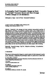
Figure 1. Decomposition of the 3-D angular velocity vector Q into a component OJ in the (x,y) plane and a component p along the z-axls, In the bottom right panel is represented the velocity field produced by the generic rotation Q. In the left and right panels are represented the velocity fields produced by the rotation components p and OJ, respectively.
of the simulated 3-D angular velocity. Even though several sources of information have been found to influence perceived 3-D angular velocity (2-D velocity magnitude, Kaiser & Calderone, 1991; edge transition rate, Kaiser & Calderone, 1991; visual texture, Norman & Todd, 1994; object size, Kaiser, 1990; deformation ofcontours, Cortese & Andersen, 1991, and Norman & Todd, 1994), the purpose of the present paper was to study the perceptual effect of the defcomponent of the velocity field in stimulus displays in which all the other sources of information have been controlled.
HEURISTIC DERIVATION OF 3-D ANGULAR VELOCITY FROM THE FIRST-ORDER OPTIC FLOW For the purposes of the present discussion, the relevant properties of def can be discussed with reference to a planar patch. The orientation of a planar patch in 3-D space can be described in terms of its slant, a (the tangent of the angle between the line of sight or z-axis and
the normal to the patch), and its tilt, rtthe angle between the projection of the normal to the patch onto the x-y plane and the horizontal or x-axis). The generic angular velocity can be decomposed into two components (see Figure 1): one parallel (w) and one orthogonal (p) to the image plane. The global angular velocity, n, therefore, can be expressed as
n = ~ w2 + p2
.
(I)
It can be shown that the def component of the optic flow is equal to the product of the slant of the patch, a, and the component of angular velocity, w, parallel to the image plane (see Domini et aI., 1997):
def= oto.
(2)
Figure 1 illustrates the relation between defand the a and wcomponents ofthe global velocity vector (see also Koenderink, 1986). The bottom panel shows a linear velocity field produced by the orthographic projection of a planar patch rotating about a generic axis. In this figure, the global velocity field has been decomposed into two
3-D ANGULAR VELOCITY DISCRIMINATION
Figure 2. Velocity fields produced by the rigid rotation of a planar patch about the vertical axis. Top panel: The velocity field generated by a constant 3-D angular velocity and a slant of 20·, Bottom panel: The velocity field generated by a constant 3-D angular velocity and a slant of 80·.
components: the component representing the magnitude of rotation about an axis orthogonal to the image plane (p) (top right panel), and the component representing the magnitude of rotation about an axis parallel to the image plane ((0) (top left panel). A rotation about an axis orthogonal to the image plane produces 2-D rigid motion, whereas a rotation about an axis parallel to the image plane produces 2-D nonrigid motion (and parallel trajectories). We can distinguish between rigid and nonrigid 2-D motion by considering the vectors depicted in the figure. Even though these vectors represent instantaneous velocities, they can be thought of as 2-D displacements associated with a small 3-D rotation. If the projected 2-D distance between any two points of the planar surface remains constant during the rotation, then the 2-D motion is rigid. Conversely, if this distance changes, then the 2-D motion is nonrigid. With this definition, we can think of defas a measure of the amount of 2-D nonrigidity produced by the orthographic projection of a 3-D rigid motion. As can be seen in Figure 1, de/is unaffected by the
749
magnitude ofthe angular velocity component p, whereas it increases with increasing (0. The relationship between def and slant is illustrated in Figure 2, which shows the velocity field produced by the orthographic projection ofa planar surface rigidly rotating about the vertical axis. At the beginning of a rotation of 80°, the surface is slanted 20° about the x-axis (top panel). (Note that the velocities ofpoints closer to the vertical rotation axis, at the top, are slower than those farther from the rotation axis.) During the rotation, the slant of the surface increases. If the angular velocity is constant, then the increase of slant produces an increase of def( see Equation 2). In Figure 2, the increase of defis revealed by the larger magnitude of 2-D nonrigidity at the end of the rotation (bottom panel) relative to the magnitude of2-D nonrigidity at the beginning of the rotation. It is important to realize, however, that def does not uniquely specify the two parameters by which it is defined (i.e., the slant, a, and the rotational component parallel to the image plane, (0). The same def, in fact, is compatible with a one-parameter family of solutions for a and (0, which can be represented by the loci of points of the hyperbola described by Equation 2. Since there is no evidence that the perceptual system uses the second-order temporal derivatives ofthe optic flow (Todd, Akerstrom, Reichel, & Hayes, 1988; Todd & Bressan, 1990; Todd & Norman, 1991; see also Domini et al., 1997, and Liter, Braunstein, & Hoffinan, 1994) that are necessary to uniquely recover the projected (0, we hypothesize that the perceived component of angular velocity parallel to the image plane ((0') is chosen heuristically as a monotonically increasing function of def(see Domini, Caudek, & Gerbino, 1995; Domini et al., 1997): (3) The component of angular rotation about the line of sight (p) can be correctly derived from the first-order properties of the optic flow (Hoffinan, 1982). Therefore, we hypothesize that the perceived component of angular velocity orthogonal to the image plane, p', is at least an increasing function of the simulated component: (4) Finally, we hypothesize that the perceived global angular velocity is derived by combining the perceived components p' and (0' as follows: (5) For three points, def can be computed from the 2-D coordinates of the orthogonal projection of the points and their instantaneous 2-D velocities (see Domini et aI., 1997). For more than three points not lying on a planar surface, the defvalues for all triplets of points form a distribution. The mean de/value can be very sensitive to extreme values; the median value is more representative of the central tendency of the defvalues. Ifwe hypothesize that the median defvalue is used, then the model described by Equation 5 both accounts for findings on the percep-
750
DOMINI, CAUDEK, TURNER, AND FAVRETTO
tion of3-D angular velocity discussed below and makes several predictions that were explicitly tested in the experiments presented in this paper. Previous researchers have found that perceived angular velocity is very close to the simulated angular velocity. Kaiser (1990) investigated the perception of3-D angular velocity by considering the discrimination thresholds for the angular velocities of two simultaneously viewed solid cubes and other shapes. Kaiser found that observers were able to discriminate angular velocities with a competence near that for linear velocities (McKee, 1981) but that perceived velocity was biased by the number of faces revealed during rotation and by object size (i.e., smaller objects had to rotate faster than larger objects to rotate with perceptually the same velocity, and the same was true for objects with a smaller number of faces). Kaiser and Calderone (1991) extended these findings by considering rotating simulated spheres defined by either random or regularly spaced texture elements on their surfaces. Again, they found that "the motion parameter accounting for most of the variance in observers' judgments is the true angular velocity, o: Whereas extraneous spatiotemporal characteristics of the stimuli shift PSEs [points of subjective equality], these shifts are relatively minor" (p. 433). Further results supporting the hypothesis that perceived angular velocities are a function of the simulated angular velocities are provided by Petersik (1991). In three experiments, the subjects compared the angular velocities of two rotating spheres of random dots. The results agreed with the results ofKaiser and Calderone (1991): The PSEs were close to the objective equality. Furthermore, the PSEs obtained from the direct estimates (judgments of the amount of angular rotation) of the 3-D angular velocities of the spheres agreed with the PSEs from the indirect estimates (comparing the angular velocity of two simultaneously viewed rotating spheres). In a third experiment, Petersik varied the sphere diameter and showed that, although rotation judgments are biased by mean linear velocity, they are not likely to be made solely on the basis of that information. In summary, the psychophysical data provided by these studies indicate a good sensitivity to the higher order parameter defined by 3-D angular velocity. Two principal findings summarize the data of Kaiser and Calderone (1991) and Petersik (1991): First, the angular velocities of two rotating spheres are correctly matched by the subjects, almost independently ofthe sizes of the spheres. Since the sizes are correlated with the 2-D velocities, it seems that the subjects' judgments are not influenced by the 2-D velocities. Second, the direct estimation ofthe angular velocity ofa rotating sphere is a monotonically increasing function of the simulated angular velocity. Both of these results can be accounted for by the model described by Equation 5. The median of the de! values for each triplet of feature points produced by clouds of dots contained within spheres having different diameters and the same angular velocity is the same. In fact, changing the size of a 3-D object isotropically leaves the slants of all the triplets of feature points unchanged. Thus, in-
creasing a sphere's radius and keeping 3-D angular velocity constant have no effect on the median del, and 3-D angular velocity derived by Equation 5 is not affected by such a manipulation. This is true whether the object's optic flow results from a perspective or an orthographic projection (see the Appendix). On the other hand, increasing the simulated 3-D angular velocity of such spheres increases the median del, since it leaves the median slants ofall the triplets of feature points unchanged but increases the component of angular velocity parallel to the image plane (see Equation 2). Thus, unless the axis of rotation is changed to decrease the component of angular velocity along the line of sight p, according to Equation 5, increasing the simulated 3-D angular velocity must increase the perceived 3-D angular velocity for these spheres. There are two predictions of Equation 5 for perceived 3-D angular velocity Q', which we directly tested in the following experiments. First, if angular velocity Q and the component in the image plane mare constant, but slant a increases or decreases, the perceived angular velocity should increase or decrease as well. The prediction holds whether p, the component of angular velocity around the line of sight, is zero or nonzero. As long as p is constant, the predicted p' is also constant, so that increasing de! should increase perceived angular velocity. Second, if the average slant a increases or decreases and it is possible to manipulate angular velocity min such a way that the product ofthe two is constant, and p is constant, then perceived 3-D angular velocity should also be constant. Thus, we can predict a dissociation between simulated and perceived angular velocity: Under certain conditions, observers will see a simulated constant angular velocity as varying and, under other conditions, a simulated varying angular velocity as constant. In the first experiment, we tested the effect of varying deformation on the perceived angular velocity of spheres and ellipsoids rotating about axes in the image plane (i.e., where p is zero). In the second experiment, de! and angular velocity were manipulated independently on planes rotating about axes in the image plane. In the third experiment, the axes of rotation were no longer in the image plane, and the ratios of maximum to minimum de! and maximum to minimum angular velocity were controlled.
EXPERIMENT 1 In the previous research discussed above, the shapes used to study the perceived 3-D angular velocity were spheres (Kaiser & Calderone, 1991; Petersik, 1991). Dots in a spherical volume define an isotropic structure, since the points are spread with the same probability in all directions. On the other hand, dots in the volume of an ellipsoid define an anisotropic structure, since the dots are spread with greater probability in the direction of the major axis. For points in a spherical volume, the median de! is fairly constant over 1800 of rotation at a constant angular velocity. If the original dots are placed isotropically over the volume, subsequent rotations do not change the average slant calculated over all the triplets of dots;
3-D ANGULAR VELOCITY DISCRIMINATION
0.5
Ellipsoid Sphere
-
0.4
rn -..
'C
--...
as 0.3
CI)
'C
c: 0.2
as
:s
CI)
::E 0.1 0.0 0
90
180
Angular Rotation (deg) Figure 3. Median def values for all the triplets of 20 dots randomly distributed in a spherical volume and for all the triplets of 20 dots randomly distributed in an ellipsoidal volume, as a function of3-D angular rotation. The ratios ofthe three axes of the ellipsoid to the diameter ofthe sphere are 3:1, 0.1:1, and 1:1. The ellipsoid was originally positioned with the 3: 1 axis along the zaxis (0° of rotation), the 0.1: 1 axis along the x-axis, and the 1:1 axis along the y-axis. In every frame transition, the two shapes rotated 1° about the y-axis. The figure indicates that, unlike the median def of the ellipsoid, the median def of the sphere is roughly constant from frame to frame.
thus, the median defvalue is not greatly affected by the rotation (see Equation 2). This is not true for objects with anisotropic dots distributions; the distribution of slant values calculated over all triplets of dots is affected by the orientation of the object relative to the line of sight. Therefore, the median defwill vary with the amount of rotation for an object with a finite number of axes of symmetry under a generic rotation, as shown for the sphere and ellipsoid in Figure 3. By using a spherical or ellipsoidal volume in this experiment, we could show observers displays with varying or close to constant median defvalues. If the observers' perceptions of angular velocity were affected by the median def as hypothesized, the ellipsoidal volumes were expected to be seen as varying in angular velocity more often than the spherical volumes. Beyond this, we could control the variation of the median defvalue by accelerating and decelerating the objects during different portions of their rotations. An ellipsoid with a variable angular velocity need not have the large variation in median defthat it has under a constant angular velocity. The simulated angular velocity can vary by a fixed amount while having the effect either of increasing or decreasing the median defvalue, depending on the phase of acceleration during the rotational cycle. When rotating at a constant angular velocity about a vertical axis in the image plane, the ellipsoid's median defvalues are at a maximum when its major axis is oriented along the line of sight and are at a minimum when the major axis is oriented orthogonally to the line of sight (see Figure 4).
751
If the ellipsoid is decelerated when its major axis is oriented along the line of sight (where the defvalues are at a maximum), then the defvalues will be decreased. Similarly, ifit is accelerated when its major axis is orthogonal to the line of sight, the def values there will be increased. Over the entire rotation, the range of def variation will be reduced relative to the range of def variation in a constant angular rotation. Similarly, if the ellipsoid is accelerated when the major axis is parallel to the line of sight and decelerated 90° later, the def variation is increased relative to that of a constant angular velocity. If the simulated 3-D angular velocity is the primary influence on perceived angular velocity, then given the same amount of variation in the simulated angular velocity, the probability of perceiving a variable angular velocity should not be affected by the particular phase of the cycle in which the variation occurs. If the median def is the primary influence, however, then we would expect that accelerating the object in phase to increase the range of median defwould increase reports of varying angular velocity. Similarly, accelerating the object in phase to decrease the range of median def would decrease reports of varying angular velocity. In a pilot experiment, we studied the effect of def on the ability to distinguish constant and variable angular velocity. We simulated a random-dot ellipsoid rotating at either a constant or a variable angular velocity Q. The constant angular velocity produced a defvariation in each stimulus display as indicated in Figure 3. The varying angular velocity was computed to produce a constant def for each stimulus display. In these conditions, ifthe main determinant of the perceived angular velocity Q' were the simu_ _ _ _ _ Maximum deformation Minimum deformation
900
----------- ------
x
co z Figure 4. Schematic representation of an ellipsoidal volume in two moments ofits rotation. The median defproduced by the dots contained within the volume of the ellipsoid is at its maximum when the major axis of the ellipsoid is parallel to the line of sight (z-axis) and is at its minimum when its major axis is parallel to the x-axis.
752
DOMINI, CAUDEK, TURNER, AND FAVRETTO
YAY Phase 1 CAY VAY Phase 2
U
1.4
:c5l
1.3
(U
..:.. 1.2
~ (,) o iii
1.1
>... (U
"3 0.9 0)
«C
0.8 0.7t-----.--------,,--------,,------, 360 90 180 270 o
Angular Rotation (deg) Figure 5. The 3-D angular velocities over the full rotation in each condition of Experiment 1. The sphere and ellipsoid underwent the same velocity variations. For the ellipsoid, the VAV Phase 1 modulation increased the range of defvariation, whereas the VAV Phase 2 modulation decreased it.
lated angular velocity, then the judgments should be correct; if the main determinant of the perceived angular velocity were del, then the judgments should not be correct. The results of this pilot experiment provided no evidence that def influenced perceived angular velocity, since, in general, the judgments of the observers were correct. This failure of defto influence the judgments of perceived angular velocity was probably due to the deformation of the projected contours of the ellipsoid. This interpretation is supported by the data of Cortese and Andersen (1991), who found that the information provided by the deforming silhouettes of rotating objects is sufficient for the perceptual derivation of angular velocity. In our stimuli, then, the deformation of the 2-D contours could have overridden the effect of de! In this first experiment, we wanted to see if def could be made more salient than in the pilot experiment, to influence the judgments of perceived 3-D angular velocity even when the stimuli provided enough information for veridical judgments (i.e., contour deformation and texture gradients). In this experiment, we simulated randomdot ellipsoids and spheres rotating with either a constant or a varying angular velocity. There were two conditions with varying angular velocity for the ellipsoids. In one condition, the simulated angular velocity was accelerated so as to increase the range of median def relative to the constant angular velocity condition by 20% (varying angular velocity (VAV) Phase 1 condition; see Figure 5). In the second condition, the simulated angular velocity was accelerated so as to decrease the range of defrelative to the constant angular velocity condition by 20% (VAV Phase 2 condition; see Figure 5). We predicted that the observers would judge the ellipsoid to be rotating with a varying angular velocity in the VAV Phase 1 condition more often than in the VAV Phase 2 condition, in accordance with the defmodel.
Rotating spheres were shown either rotating at a constant angular velocity or undergoing the same acceleration and deceleration patterns as the ellipsoids. Since, for a sphere, the median slant values of every triplet of points remain constant during rotation, the median defis proportional to the simulated angular velocity (see Equation 2). Therefore, we predicted that the performance should be closer to veridical for the sphere than for the ellipsoid. Method Subjects. Thirteen University of Trieste undergraduates participated in this experiment. All ofthem were naive to the purpose of the experiment. All subjects had normal or corrected-to-normal vision. They were not paid for their participation. Apparatus. The stimuli were presented on a high-resolution color monitor (1,280 X 1,024 addressable locations), under the control ofa Silicon Graphics IRIS workstation. The screen had a refresh rate of 60 Hz and was approximately photometrically linearized. Given the on-line calculations of the display, the actual frame rate was 58 frames/sec. An anti-aliasing procedure was used: For point-light locations falling on a pixel boundary, the screen luminance was proportionally adjusted in the relevant addressable locations. The graphics buffer was 8 bits deep (256 gray levels). The subjects viewed the displays through a reduction screen that reduced the field of view to a circular area with a diameter 2° of visual angle. The eye-to-screen distance was 1.1 m. Design. Twovariables were studied in this experiment: (I) shape (sphere vs. ellipsoid) and (2) angular velocity variation (constant angular velocity [CAY], YAY Phase I, and YAY Phase 2). All variables were within subjects. Each subject viewed 10 presentations of the six conditions in one block, with the order of all trials completely randomized. Twelve additional trials were presented at the beginning of each experimental session to familiarize the subjects with the stimulus displays. Stimuli. A stimulus display consisted of20 high-luminance dots moving on a low-luminance background. The horizontal motions of the dots simulated an orthographic projection of dots undergoing a continuous rotation in 3-D (360°) about the (vertical) y-axis. The dots were randomly distributed within the volume of either a sphere or an ellipsoid. The diameter of the sphere measured 2° of visual
3-D ANGULAR VELOCITY DISCRIMINATION
-0)
dition. In the VAV Phase 2 condition, the range of del was 20% smaller than the range of def ui the CAY condition. Procedure. All subjects were run individually in one session. The subjects were instructed to judge whether the simulated objects appeared to rotate in 3-D with a constant angular velocity. In each trial, the subjects provided their judgments by a keypress. Viewing was monocular, and head and eye motions were not restricted. The experimental room was dark during the experiment. No restriction was placed on viewing time. No feedback was given until after the experiment was completed.
10
c
's, ...m
?-eI) - Q) -eI) °c
8 6
"'0
Q)Q.
.eel) EQ)
::Ja:
4
Z
c m Q) :ii:
753
2
o VAV Phase 1
CAV
VAV Phase 2
def Variation Figure 6. The mean number of trials (out of 10 possible) in which the observers reported a varying angular velocity in each condition of Experiment 1. Vertical bars represent one standard error.
angle. The ratios of the three axes of the ellipsoid to the diameter of the sphere were 3: I, I: I, and 0.1: I. At the beginning of the rotation, the ellipsoid was oriented so that its smallest axis was parallel to the x-axis of the projection plane (the horizontal axis) and its major axis coincided with the z-axis (the line of sight). Each stimulus display was contained within a circular "window" with a diameter equal in size to the diameter of the sphere. Both the sphere and the ellipsoid rotated with either a constant or a variable angular velocity. The range of angular velocity for both spheres and ellipsoids is shown in Figure 5. All displays simulated continuous 360 0 rotation until terminated by the subject's response (365 frames were needed to show the full rotation, on average). The CAY condition simulated rotation at a constant angular velocity of 1.03 rad/sec. For this condition, deJremained approximately constant in the case of the spheres. On the other hand, def varied for the ellipsoids as indicated in Figure 3. The two other conditions simulated rotation at a variable angular velocity. The VAV Phase I and Phase 2 conditions were created by manipulating the phase of the acceleration-deceleration cycle for each stimulus display (see Figure 5). The ranges of simulated angular velocities for both conditions were identical. For the spheres, the range of variation of deJin the VAV Phase I condition was identical to the range of variation of deJin the VAV Phase 2 condition. DeJ was computed by calculating the median def of all triplets of points in each pair of successive frames. For the ellipsoids, the VAV Phase I and VAV Phase 2 conditions were created as follows. For the VAV Phase I condition, when the ellipsoids were oriented with their major axis parallel to the z-axis, the velocity was increased (see Figure 4). This produced a larger de! When the ellipsoids were oriented with their major axis orthogonal to the z-axis, the velocity was decreased, producing a smaller de! This manipulation increased the range of deJvalues in the whole rotation cycle relative to the CAY condition. The VAV Phase 2 condition was produced in the opposite fashion. When the ellipsoids were oriented with their major axis parallel to the z-axis, then the velocity was decreased. This produced a smaller def. When the ellipsoids were oriented with their major axis orthogonal to the z-axis, the velocity was increased, producing a larger de! In this way, the range of def values in the whole rotation cycle was decreased relative to the CAY condition. For the ellipsoids, in the VAV Phase I condition, the range of del was 20% larger than the range of del in the constant velocity con-
Results The mean number of times (out of 10 repetitions) that the subjects reported a varying angular velocity for each condition is shown in Figure 6. On the average, the subjects were 76% correct, reporting a varying angular velocity in 76% ofthe trials in which angular velocity varied and reporting a constant angular velocity in 75% of the trials in which angular velocity was constant. The mean percent correct for all sphere conditions was 85% and for the ellipsoids was 68%. We transformed the frequency of reporting a varying angular velocity for each condition by an arcsine transformation (Winer, 1971). A 2 (shape: sphere, ellipsoid) X 3 (angular velocity variation: CAY, VAVPhase 1, VAV Phase 2) within-subjects analysis of variance (ANOVA) was run on the arcsine-transformed frequency data. Most importantly, the angular velocity variation condition had a significant effect and accounted for the most variance [F(2,I4) = 90.89,p < .001, ro2 = .61]. A planned comparison between the VAV Phase 1 and VAV Phase 2 conditions on the ellipsoids alone showed that, in the VAV Phase 1 condition, the tendency to report a varying angular velocity was significantly higher (87.5%) than in the VAV Phase 2 condition (45.0%) [F(l,7) = 31.12,p < .001]. On the other hand, for the sphere, a planned comparison between the VAV Phase 1 and VAV Phase 2 conditions did not show a significant difference [F(l,7) = 2.98, n.s.]. The interaction between shape and the angular velocity variation was significant, as can be seen in Figure 6 [F(2,I4) = 6.87,p < .01, ro2 = .07]. As expected, the frequency ofreporting a varying angular velocity in the VAV Phase 2 condition was much greater for the sphere displays than for the ellipsoid displays. As a result, the main effect of shape was also significant [F(l,7) = 6.0I,p < .05, ta? = .03]. The sphere was more frequently reported as varying in angular velocity (66% on the average) than was the ellipsoid (53% on the average). Even though we expected that the frequency of reporting a varying angular velocity for the ellipsoid should be greater in the CAY condition than in the VAV Phase 2 condition, a planned comparison between these conditions did not reveal a significant difference [F(l,7) = 2.35, n.s.]. Discussion The subjects performed quite well on the sphere displays, missing approximately 22% when the angular velocity was constant and 10% when the angular velocity was varying. This was as predicted since, for the sphere,
754
DOMINI, CAUDEK, TURNER, AND FAVRETTO
the variations in def correlated with the variations in 3-D angular velocity, and p was equal to zero. The VAV Phase I and Phase 2 displays for the sphere were identical with respect to the variation in def( except for a phase shift in the temporal sequence of the stimulus display), and the tendency to report a varying angular velocity was quite similar in both conditions. However, for the ellipsoid, only in the VAV Phase 1 condition was the tendency to report a varying angular velocity quite high. On the other hand, in the VAVPhase 2 condition, only 45% of the displays were seen correctly (i.e., with the angular velocity varying). Even though the range of angular velocity variation was the same as in the VAV Phase 1 condition, accelerating and decelerating in order to minimize defvariation had the predicted effect of increasing the tendency to perceive a constant angular velocity. When the ellipsoid rotated at a constant angular velocity, defwas not constant, yet the subjects reported a constant angular velocity on approximately 73% of the trials. It seems that the changing texture density and the (partially available) contour information were able to override the changing definformation and give a percept of a constant angular velocity. In Experiment 2, these characteristics were controlled, in order to further test the heuristic derivation of 3-D angular velocity described by Equation 5.
EXPERIMENT 2 For the shapes of Experiment I, the variation in 3-D angular velocity was accompanied by variations in the shape of the contour and in the texture density in the display. By using a planar surface whose edges extend beyond the visible window and by controlling the density of the dots on the surface, both contour and density cues can be controlled. The predictions of the heuristic model described by Equation 5 are that angular velocity will be perceived to be constant if def and p are constant. If p is constant and def varies, the perceived angular velocity should vary. By using rotation axes that are in the image plane, p was set equal to zero in all conditions in this experiment. Defand ro, however,were varied independently ofeach other. Varying ro in this case is equivalent to varying the surface's 3-D angular velocity n since the other component, p, is zero. Defwas varied during a rotation in two ways: either by varying ro(ifthe slant o was constant) or by varying (J" (if the angular velocity component mwas constant). It is possible that the absolute amount of defvariation necessary to affect angular velocity perception is a function of the average angular velocity present. To determine any possible effect of the mean angular velocity, we manipulated the mean 3-D angular velocity of the surface by decreasing the amount of rotation between frames, while increasing the number of frames and keeping the frame rate constant. This kept the total amount of 3-D rotation constant. While the 2-D velocities were not explicitly manipulated as a variable in this experiment, the variation in 2-D
velocity in each condition was also computed. The 2-D velocity tended to have a large variation when the 3-D angular velocity varied and tended to have a smaller variation when the 3-D angular velocity was constant. The implications of this will be discussed below.
Method Subjects. Eighteen University of Trieste undergraduates participated in this experiment. All of them were naive to the purpose of the experiment, had normal or corrected-to-normal vision, and volunteered their time. Apparatus. The apparatus was the same as in Experiment I. Design. Three variables were studied in this experiment: (I) mean angular velocity (.044, .029, and .022 rad/sec), (2) 3-D angular velocity variation (constant vs. variable), and (3) defvariation (constant vs. variable). All variables were within subjects. Each subject viewed 10 presentations of the 12 different conditions; the 120 trials were presented in a random order. Twelve additional trials were presented at the beginning of each experimental session for practice. Stimuli. The stimuli were 40 high-luminance dots moving on a low-luminance background. The motions of the dots simulated an orthographic projection of a planar surface oscillating in 3-D about an axis in the projection plane. Each stimulus display was contained within a circular "window" with a diameter of 2°of visual angle to prevent changes in the projected contours of the simulated surfaces from being visible. The dots were randomly distributed with uniform probability density over the projection plane. Dot density was controlled by randomly deleting (or adding) dots to keep the number of dots constant in each frame of the stimulus display. During each oscillation cycle, simulated 3-D angular velocity and defwere kept constant or varied independently. This created four conditions: constant angular velocity/constant def(denoted Cvel Cdej), varying angular velocity/constant def(denoted Vve/Cdej), constant angular velocity/varying def(Cvel/Vdej),and varying angular velocity/varying def(VvelVdej)' These were created by changing the orientation of the plane relative to the axis ofrotation across conditions and by varying or maintaining the angular velocity within a condition. Figure 7 shows the orientation ofthe planar surfaces relative to the axis of rotation in each experimental condition. The tilt of the axis of rotation (and, therefore, of the planar surface) was determined randomly on each trial from 0° to 360°. The initial slant rr of the surface was always 8 [i.e., tan (82.9°)]. When the axis of rotation is almost perpendicular to the surface, with an initial slant close to tan (90°), a small rotation induces very little slant change. Thus, by keeping the angular velocity constant in such a condition and with a small rotation angle, we can produce a nearly constant de! Conversely, if the angular velocity varies, then the defwill also vary. On the other hand, when the axis of rotation is almost parallel to the surface, with an initial slant close to tan (90°), a small rotation induces a very large slant change. Thus, if the 3-D angular velocity is constant in such a condition, the defwill still vary; but the def can also be kept constant if the 3-D angular velocity varies in such a way that the product of OJ and G is kept constant. In the Cvel/Cdejcondition (Figure 7a), the axis of rotation was almost perpendicular to the planar surface. In this way, a 6° rotation produced a negligible change of the slant of the surface. Therefore, defwas nearly constant since the 3-D angular velocity was constant (see Equation 2). The defvaried over the course of the display by 0.3%,0.7%, and 0.5% in the slowest, medium, and fastest angular velocity conditions, respectively. The projected 2-D velocity of each dot was also nearly constant during the time course of a stimulus display, varying by 0.5%, 0.3%, and 0.5% in the three angular velocity conditions. In the Vvel/Cdej condition (Figure 7b), the axis of rotation was contained in the planar surface. A 5.6° rotation produced a large change of the slant of the surface, but we compensated for the slant variation with a variation of the 3-D angular velocity in order to keep
3-D ANGULAR VELOCITY DISCRIMINATION
755
Angular Velocity Constant
Variable
c:
m
iii c: o
o
-
a
b
Go)
"C
c
d
Figure 7. Orientation of the simulated planar surfaces relative to the axis of rotation in each condition of Experiment 2. the product ofthe two constant. Therefore, defwas constant. The projected 2-0 velocity of each dot varied during the time course of a stimulus display by 494%, 499%, and 494% in the three angular velocity conditions. The 3-0 angular velocity varied by 472%,478%, and 483% in the same conditions. In the CvelVdef condition (Figure 7c), the axis of rotation again was contained in the planar surface. In this way, a 60 rotation produced a large change of the slant of the surface. Therefore, defwas variable since the slant was variable. The defvalues varied by 622%, 628%, and 630% in the slowest, medium, and fastest angular velocity conditions, respectively. The projected 2-0 velocity ofeach dot, however, was very nearly constant, never varying more than 0.9%, In the VvelVdef condition (Figure 7d), the axis of rotation again was almost perpendicular to the planar surface. In this way, a 5.80 rotation produced a negligible change of the slant of the surface. But since the 3-0 angular velocity was variable, defwas also variable. The projected 2-0 velocity ofeach dot was also variable in this condition. The 3-0 angular velocity varied by 667%,710%, and 721%, the defvalues varied by 664%, 704%, and 718%, and the 2-0 velocity varied by 587%, 646%, and 684% in the slowest, medium, and fastest 3-0 angular velocity conditions, respectively. In the variable angular velocity conditions, the total amount of rotation was not the same as in the constant angular velocity conditions because of the necessary manipulations to control de! In Figures 8, 9, and 10 are shown the 3-0 angular velocity, de! and 2-0 velocity for each stimulus type for each frame transition in the 0.044 rad/sec condition. The 2-0 velocity plot indicates the ratio between the 2-0 velocity ofa dot in a frame transition and its minimum 2-0 velocity in a frame transition across the whole stimulus sequence. We used this measure since the absolute magnitude of 2-0 velocity is different for each dot of a display, but this ratio is the same for all dots in each frame transition. Since the simulated angle of rotation was very small in all conditions, when the 3-0 angular velocity was constant, the 2-0 projected velocity was nearly constant for each dot over the course of a display. Conversely, when the 3-0 angular velocity was variable, the 2-0 projected velocity for each dot was also variable over the course of a display.
Each stimulus display had 40, 60, or 80 frames. Varying the number offrames while keeping the magnitude of rotation constant varied the average angular velocity for a display: 0.044, 0.029, and 0.022 rad/sec in the 40-, 60-, and 80-frame conditions, respectively. Procedure. The procedure and instructions were the same as in Experiment I.
Results The mean number of times (out of 10 repetitions) that the subjects reported a varying angular velocity in each condition is shown in Figure 11. Overall, the mean percent correct across conditions was 61.7%. A 3 (mean angular velocity: 0.044, 0.029, 0.022 rad/ sec) X 2 (def: constant, varying) X 2 (angular velocity variation: constant, varying) within-subjects ANOVA was run on the arcsine-transformed frequency data. The effect of defwas significant and accounted for the highest proportion ofvariance [F(l,17) = 122.25,p < .001,0)2 = .64]. When def varied, the frequency of reporting a varying angular velocity was significantly higher (76.3%) than when defwas constant (20.8%). The effect oO-D angular velocity was also significant, though it accounted for a negligible portion ofthe variance [F(l,17) = 19.19, P < .001, 0)2 = .02]. The frequency of reporting a varying angular velocity was higher when angular velocity did vary (53%) than when angular velocity was constant (44%). The effect of the mean angular velocity was not significant [F(2,34) < 1.0]. The interaction between defand velocity was significant [F(l,17) = 8.29,p < .01, 0)2 = .02]. As can be seen in Figure 11, the effect of velocity was greater when def was constant; when defwas varying, the subjects nearly always reported a varying angular velocity, whether or
756
DOMINI, CAUDEK, TURNER, AND FAVRETTO 0.1
--&-Cds,/Cvel - - Cds,lV vel
Ul :c 0.08
-vds,/cvel
ttl
- - V do,/vvOI
~
~0.06 CJ
o
D angular velocity was found when defwas constant, but it was very small relative to the effect of de! These results were obtained for rotations about a rotation axis in the image plane. The heuristic derivation of3-D angular velocity described by Equation 5 was formulated to take into account generic rotation axes. Experiment 3 tested the model in the more generic case.
~ 0.04
EXPERIMENT 3
~
ttl
:; 0.02 C)
I:
«
0+----,.--,------,-,--.---,,..--,-----,
o
5
10 15 20
25 30
35
40
Frames Figure 8. The 3-D angular velocity for each condition of the 0.044 radlsec stimulus sequence of Experiment 2.
not the velocity was actually varying. The interaction between defand the mean angular velocity was also significant, though it accounted for a negligible portion of the variance [F(2,34) = 5.03, P < .05, (02 = .004]. As mean angular velocity decreased, the difference between the effects of constant and varying defbecame more pronounced: At 0.044 rad/sec, in the constant def condition, the mean frequency ofreporting varying angular velocity was 25%, and in the variable defcondition, the mean frequency was 73%. At 0.022 rad/sec, the mean frequencies were 18% and 78%, respectively. Discussion The results of Experiment 2 tend to support the predictions of Equation 5: Under certain conditions, the observers reported a varying angular velocity when the angular velocity Q was constant and,under other conditions, when Q varied. When defwas constant, the observers were more likely to report a varying angular velocity correctly, but they were unable to distinguish constant from varying angular velocity when def was varying. When def varied, the observers reported a varying angular velocity on approximately 76% ofthe trials, though the angular velocity was varying on only half of the trials. Thus the observers tended to perceive a varying angular velocity when defvaried, but not necessarily when angular velocity varied. Similarly, the reports of varying angular velocity were not primarily determined by the 2-D velocities: The 2-D velocities ofeach dot were nearly constant over the course of a display when 3-D angular velocity was constant, and they varied when 3-D angular velocity varied. It is possible that when defwas constant, either the variation in 2-D velocity or the variation in 3-D velocity allowed the observers to report a varying angular velocity more correctly. The effect was small, however, and accounted for only 2% of the total variance. In conclusion, in Experiment 2, the angular velocity and the definformation were decoupled, and the observers' reports of perceived variable angular velocity were predicted for the most part by de! An effect of varying the 3-
In the heuristic derivation of3-D angular velocity described by Equation 5, perceived 3-D angular velocity is a function both of def and of p, the component of image velocity around the line of sight. In Experiments I and 2, only defwas varied, as p was kept constant at zero. In Experiment 3, in one condition, p was constant but nonzero, and, in another condition, it varied over the course of a display. If defis held constant while p is varied, a varying angular velocity should still be perceived. Although Experiments I and 2 demonstrated that varying def can cause a varying angular velocity to be perceived, the amount of defvariation was not systematically manipulated. If the perceived angular velocity is a monotonically increasing function of def as assumed in the model, then increasing the def variation should increase the tendency to report a varying angular velocity. Similarly, increasing the variation in p should increase the tendency to report a varying angular velocity. To test this prediction, in Experiment 3, the ratio ofmaximum to minimum defwithin a display could be one of three values p was held constant, or the ratio of maximum to minimum p within a display could be one ofthree values and defwas held constant.
Method Subjects. Six University of Trieste undergraduates participated in this experiment. All of them were naive to the purpose of the experiment, had normal or corrected-to-normal vision, and volunteered their time. Apparatus. The apparatus was the same as in Experiment I.
2.5
--&- Cds,/Cvel - - Cds,/Vvel
--
2
Vdo,/c.el - - Vds,/Vvel
:cen 1.5 ttl
~
Q)
'C
0.5 O+---r-..,----r--,--,----,---,---,
o
5
10 15 20
25
30 35
40
Frames Figure 9. The defvalues for each condition ofthe 0.044 radlsec stimulus sequence of Experiment 2.
3-D ANGULAR VELOCITY DISCRIMINATION
6
--e-
Cdo,/CvoJ
- - Cdo,/VvOI
o 5
:;:
----If--
lU
Vdo,/C vol
- - Vdo,/Vvol
a: 4 >-
-
'0 3
o
Ql
>
2
sition in which deJwas maximum, the screen was blackened for 200 msec. The display was repeated until the subjects provided their judgments. Angular velocity took on the values of0.569, 0.628, and 0.648 rad/sec for the simulated deJratios of3, 5, and 7, respectively. In the Vvel/Cdejcondition, the orientation of the axis of rotation on each trial was determined by randomly choosing one axis from the previously defined set. In each trial, the planar surface was rotated around the axis to have an initial slant equal to 1 [tan (45°)]. To obtain a constant value of def, the increment in the angle of rotation for each frame transition was the following:
~a=
C
C\I
O+--r---.---,---,.-----r--..--~-~
o
5
10
15 20
25 30 35
40
Frames Figure 10. Ratio between the 2-D velocity of a point in each frame transition and its minimum 2-D velocity over the course of a display for each condition of the 0.044 rad/sec stimulus sequence of Experiment 2.
Design. We used two combinations of angular velocity and def, and three possible ratios between the maximum and minimum values of either 3-D angular velocity or deJin a display. The two combinations of angular velocity and defwere constant angular velocity/variable def (CveINder) and variable angular velocity/constant deJ(Vve/Cdej)' If 3-D angular velocity remained constant in a display, the ratios between the maximum and minimum def could be 3, 5, or 7. In the same way, if def remained constant, the ratios between the maximum and minimum 3-D angular velocity could be 3,5, or 7. Each subject viewed 80 presentations in random order of the six conditions. Twelve additional trials were presented at the beginning of each experimental session for practice. Stimuli. The stimuli were 40 high-luminance dots moving on a low-luminance background. The motions of the dots simulated an orthographic projection of a planar surface undergoing 3-D oscillation. Twenty-five possible axes of rotations were chosen from 34 generated using the same procedure as Braunstein, Hoffman, and Pollick (1990): 34 points were chosen evenly spaced on the surface of a sphere,and the axes of rotation were defmed by connecting each of these points to the center of the sphere. Of the 34 axes generated this way, 9 were almost in the image plane (their slants were larger than 81°), and they were discarded. The slant of the remaining axes ranged from 45° to 81 0, and their tilt varied between 0° and 180°. Each stimulus display simulated a rotation about an axis contained in the simulated surface. The dots were randomly distributed with uniform probability density over the projection plane (not evenly distributed over the simulated surfaces). Dot density was manipulated as before to keep the number of dots constant in each frame of the stimulus display. Each stimulus display was contained within a circular "window" with a diameter of 2° of visual angle. Two variables were manipulated: angular velocity and de! For each trial, they could either remain constant or vary. Two stimulus conditions were defined: constant angular velocity/variable deJ( denoted Cve/Vde! ) and variable angular velocity/constant deJ( denoted Vve/C de/)· In the Cve/Vde! condition, on each trial, one axis of rotation was chosen randomly from the previously defined set of axes. The planar surface was oriented parallel to the axis and with an initial slant equal to I [tan (45°)]. Each stimulus display was made up of 20 frames. The angle of rotation for each frame transition was computed using an iterative procedure so that the angular velocity was constant but the deJofthe last frame transition was 3, 5, or 7 times larger than the deJofthe first frame transition. After the frame tran-
757
deJM
(6)
a surface COS( (faxis) ,
where craxis is the slant of the axis of rotation, ~t is the temporal duration of a frame transition, and crsurface is the slant of the simulated surface. In each stimulus display, the slant of the simulated surfaces increased monotonically during the rotation. In the last frame transition, ~atook on a value that was 3, 5, or 7 times larger than the ~a of the first frame transition. This procedure produced a different number of frame transitions in different stimulus displays depending on the orientation of the axis ofrotation. The ratios between the maximum and minimum simulated 3-D angular velocities took on the values of3, 5, or 7. Consequently, the ratios between the maximum and minimum values of p took on the same values. After the frame transition in which the simulated 3-D velocity was maximum, the screen was blackened for 200 msec. The display was repeated until the subjects provided their judgments. In each display, deJtook on the values of 0.8 rad/sec for the simulated 3-D angular velocity ratios of3, 5, and 7. The average magnitude of deJfor each frame transition over 240 stimuli for the ratios between maximum and minimum deJof3, 5, and 7 in the Cve/Vdej condition is shown in Figure 12. The average magnitude of p for each frame transition over 240 stimuli for the ratios between maximum and minimum p of3, 5, and 7 in the Vvel/Cdej condition is shown in Figure 13. Procedure. The procedure and instructions were the same as in Experiment I, except that the trials were broken up into a total of four sessions of equal length.
Results The mean number of times (out of 80) that the subjects reported a varying angular velocity in each condition 10 Cl
r::
8
.~
lU
> :
til
Ql
6
-til
-VvollCdo'
Or::
~O
~~4 Ql Ea: ::J Z
r::
-&-
Cvot/Cvol
---+- Vvo,/V do'
2
~~-'I------~
lU
Ql
:!!:
--e- Cvot/Cdo'
0+----,--,----,----,---, 0.02
0.025
0.03
0.035
0.04
0.045
AngUlar Velocity (rad/s) Figure II. The mean number of trials (out of 10 possible) in which the observers reported a varying angular velocity in each condition of Experiment 2. Vertical bars represent one standard error.
758
DOMINI, CAUDEK, TURNER, AND FAVRETTO
5
- - defmax/defmln - - - defmax/defmln ..... _..... defmax/defmln
4
GENERAL DISCUSSION
=3 =5 =7
I
I
,.'
.:
/ /
1
O+---,---r---,-----r-----,
o
4
8
12
16
20
Frames Figure 12. The defvalues for each ratio between maximum and minimum defin the constant angular velocity/variable defcondition of Experiment 3, over a full display cycle.
is shown in Figure 14. On the average, the subjects were 33% correct (significantly less than chancel), reporting a varying angular velocity on 65% of the trials in which angular velocity was constant and only on 31 % ofthe trials in which angular velocity varied. The effect of maximum to minimum defratio was examined by performing a within-subjects ANOVA on the arcsine-transformed frequency data in the Cve/Vde! condition [F(2,1O) = 83.96, p < .05, (J)2 = .89]. Planned comparisons revealed significant differences between the smallest ratio condition and the next larger ratio condition [F(1,5) = 64.64, p < .05] and between the two largest ratio conditions [F( 1,5) = 17.26, P < .05]. The effect of maximum to minimum velocity ratio was examined by performing a within-subjects ANOVA on the VveI/Cde!condition. The effect of velocity ratio was not significant [F(2, 1O) = 1.83, n.s.].
The heuristic model described by Equation 5 predicts that the perception of 3-D angular velocity will not be veridical. Specifically, perceived 3-D angular velocity from optic flow will be an increasing function of the def component of the optic flow and the component of angular velocity around the line of sight. The predictions of this model were supported by the experimental results. In Experiment 1, increasing the range of defvariation increased the tendency to report a varying angular velocity, even though the actual range of angular velocity variation was unchanged. In Experiment 2, the tendency to report a varying angular velocity was much less when defwas constant than when defvaried. When defvaried, the tendency to report a varying angular velocity was very strong and was essentially unaffected by whether the simulated 3-D angular velocity varied or not. In Experiment 3, increasing the range of def variation while holding angular velocity constant increased the tendency to report a varying angular velocity. The model also predicts that a variation in p will lead to variation in the perceived 3-D angular velocity. In Experiment 3, the variation in p produced by varying the 3-D angular velocity around an axis not in the image plane did affect the tendency to report a varying angular velocity. This effect was not as large as the effect of defeven though the ratio of maximum to minimum p when p varied was the same as the ratio of def variation when def varied. Possibly the visual system might be more sensitive to defthan to p, however, and this warrants further research. There was a small effect of the simulated 3-D angular velocity found in Experiment 2: When defwas constant, varying the 3-D angular velocity did increase the tendency to report a perceived varying 3-D angular velocity. 0.4 - - PmaxiPmln = 3 - - - PmaxiPmln = 5 ............ PmaxiPmln = 7
0.35
Discussion The results confirm the findings of Experiments 1 and 2, in that perceiving a varying 3-D angular velocity depends more on the variation in def than on whether the simulated 3-D angular velocity is actually varying. The observers' reports of a varying angular velocity when def varied were in a ratio of 2 to 1 with their reports of such a percept when defwas constant but angular velocity varied. Thus, even when the axis of rotation is not in the image plane, but is more generically positioned, observers' perceptions of a constant or varying 3-D angular velocity depend on whether defis constant or varying. Moreover, we found that the increase ofboth the ratios of maximum to minimum def and the ratios of maximum to minimum p increased the tendency of reporting a varying angular velocity, even though the effect of the variation in p did not reach significance.
---... en
'C
ctI
0.3 0.25 0.2
a. 0.15 0.1 0.05
o -+--r----r--,----.------.-~-~
o
5
10
15
20
25
30
35
Frames Figure 13. The p values for each ratio between maximum and minimum 3-D angular velocity in the variable angular velocity/constant def condition of Experiment 3, over a full display cycle.
3-D ANGULAR VELOCITY DISCRIMINATION
.0)
c::
80
's,
70
> en : 0)
60
a:
30
...CU
- - 0 - Cdo,lV dBf
_Vyol/Cdef
-en o c:: 50 ... 0 O)e. .c en 40 EO) ::J
Z
c::
CU
0)
~
20 10
+--,.------.,.-----,-3
5
7
Ratio Figure 14. The mean number of trials (out of 80 possible) in which the observers reported a varying angular velocity in each condition of Experiment 3. Vertical bars represent one standard error.
On the average, however, a constant angular velocity was reported on more than 60% of the trials in which angular velocity varied while defwas constant, and a variable angular velocity was reported on more than 75% of the trials in which angular velocity was constant while def varied. Within the present stimulus parameters, this argues for a primary effect of def on 3-D perceived angular velocity, rather than the simulated 3-D angular velocity as has been claimed previously (Kaiser & Calderone, 1991; Petersik, 1991). The tendency to report a varying 3-D angular velocity did not seem to be affected by variations in the 2-D velocities of the dots in the display. In Experiment 2, the 2-D velocity varied with the simulated angular velocity, but the variation in def had the greatest effect on whether the 3-D perceived angular velocity varied. Even though the ratio of maximum to minimum 2-D velocity ofa dot over the display could be as high as 5.8, when defwas constant, 3-D angular velocity tended to be perceived as constant. Defhas been shown to affect several aspects of perceived structure from optic flow. The influence of def on the perception of rigidity in SFM displays has been studied by Domini et al. (1997). Moreover, Caudek and Domini (1998) studied the influence of def on the perception of the orientation of the axis of rotation. In both studies, they found that, in general, the perceptual judgments were not influenced by the simulated 3-D stimulus properties but depended mainly on the manipulation of de! The findings of these studies parallel the findings here, in that the ability to detect a varying 3-D angular velocity can depend on the variability of the median de! The heuristic model of Equation 5 has been tested in these experiments using stimuli with only optic flow information about the angular velocity. Other sources of information about the angular velocity can exist: In particular, the results of Experiment 1 show that the effects ofdefcan be overcome in part by texture and boundary information, which are in themselves sources of informa-
759
tion about the 3-D angular velocity (Cortese & Andersen, 1991). The extent to which these and other factors and the defin formation interact is an issue for future research . In summary, perceived 3-D angular velocity is not veridical, as predicted by Domini et al. (1997): 3-D angular velocity can be perceived to vary or to be constant somewhat independently of the simulated angular velocity, if the defand p variation is large or small, respectively. This argues against the notion that the human visual system uses an assumption of rotation at a constant angular velocity to recover structure within a mathematically correct analysis of the stimulus information, and it argues for a heuristic analysis based on the first-order optic flow. REFERENCES BRAUNSTEIN, M. L., HOFFMAN, D. D., & POLLICK, E E. (1990). Discriminating rigid from nonrigid motion: Minimum points and views. Perception & Psychophysics, 47, 205-214. CAUDEK, c., & DOMINI, E (1998). Perceived orientation of axis of rotation in structure-from-motion. Journal of Experimental Psychology: Human Perception & Performance, 24, 609-621. CORTESE, 1. M., & ANDERSEN, G. J. (1991). Recovery ers.oshape from deforming contours. Perception & Psychophysics. 49, 315-327. DoMINI, E, CAUDEK, C; & GERBINO, W. (1995). Perception of surface attitude in structure from motion displays. Investigative Ophthalmology & Visual Science, 36, 1694. DoMINI, E, CAUDEK, C., & PROFFITT, D. R. (1997). Misperceptions of angular velocities influence the perception of rigidity in the kinetic depth effect. Journal ofExperimental Psychology: Human Perception & Performance, 23,1111-1129. HILDRETH, E. (1984). The measurement of visual motion. Cambridge, MA: MIT Press. HOFFMAN, D. D. (1982). Inferring local surface orientation from motion fields. Journal ofthe Optical Society ofAmerica, 72, 888-892. HOFFMAN. D. D., & BENNETT, B. (1985). Inferring the relative 3-D positions of two moving points. Journal ofthe Optical Society ofAmerica A, 2, 350-353. HOFFMAN, D. D., & BENNETT, B. (1986). The computation of structure from fixed axis motion: Rigid structures. Biological Cybernetics, 54, 71-83. KAISER, M. K. (1990). Angular velocity discrimination. Perception & Psychophysics, 47, 149-156. KAISER, M. K., & CALDERONE, J. B. (1991). Factors influencing perceived angular velocity. Perception & Psychophysics, 50, 428-434. KOENDERINK, J. J. (1986). Optic flow. Vision Research, 26,161-179. KOENDERINK, J. J., & VAN DOORN, A. J. (1975). Invariant properties of the motion parallax field due to the movement of rigid bodies relative to an observer. Optica Acta, 22, 773-791. KOENDERINK, J. J., & VAN DOORN, A. J. (1976). Local structure of movement parallax of the plane. Journal of the Optical Society of America A, 66, 717-723. LITER, J. c.. BRAUNSTEIN, M. L., & HOFFMAN, D. D. (1993). Inferring structure from motion in 2-view and multi-view displays. Perception, 22,1441-1465. LITER, J. C., BRAUNSTEIN, M. L., & HOFFMAN, D. D. (1994). Detection of one versus two objects in structure from motion. Journal of the Optical Society ofAmerica A, 11, 3162-3166. MARASCUILO, L. A. (1970). Extensions of the significance test for oneparameter signal detection hypotheses. Psychometrika, 35, 237-243. McKEE, S. P. (1981). A local mechanism for differential velocity detection. Vision Research, 21, 491-500. NORMAN, J. E, & TODD, J. T. (1994). Perception of rigid motion in depth from the optical deformations of shadows and occlusion boundaries. Journal of Experimental Psychology: Human Perception & Performance, 20, 344-356. PETERSIK. J. T. (1991). Perception of three-dimensional angular rotation. Perception & Psychophysics, 50, 465-474. TODD, J. T., AKERSTROM, R. A., REICHEL, ED., & HAYES, W. (1988). Ap-
760
DOMINI, CAUDEK, TURNER, AND FAVRETTO
parent rotation in three-dimensional space: Effects of temporal, spatial, and structural factors. Perception & Psychophysics, 43, 179-188. TODD, J. T., & BRESSAN, P. (1990). The perception of 3-dimensional affine structure from minimal apparent motion sequences. Perception & Psychophysics, 48, 419-430. TODD,J.T., & NORMAN, J. F.(1991). The visual perception of smoothly curved surfaces from minimal apparent motion sequences. Perception & Psychophysics, 50, 509-523. ULLMAN, S. (1979). The interpretation of visual motion. Cambridge, MA: MIT Press. WINER, B. J. (1971). Statistical principles in experimental design (2nd ed.). New York: McGraw-Hili. NOTE I. The experimental data were analyzed by means of a signal detection paradigm, considering the "varying angular velocity" trials as signal trials. A d' measure was computed for each observer. The significance of d' was calculated by using Marascuilo's (1970) one-signal significance test. The results of this analysis revealed that all six d's were significantly less than zero.
APPENDIX Influence of Size and Angular Velocity on Median del of Random Dot Spheres Stimuli similar to those ofKaiser and Calderone (1991) and Petersik (1991) were simulated under a perspective projection to de-
termine their median de! Kaiser and Calderone and Petersik simulated the perspective projection of rotating random-dot spheres. For Kaiser and Calderone, the standard sphere had a diameter of 4.5° of visual angle, was made up of 400 points, and was rotated at 2.5°/frame. For Petersik, the standard sphere had a diameter of 11.2° of visual angle, was made up of50 dots, and was rotated at 3°Ifi·ame. For Kaiser and Calderone and for Petersik, the dots were positioned either inside the spheres or on their surfaces. To verify that median de/is affected by angular velocity and not by the size of the sphere, we ran a computer simulation on a set of nine spheres made up of 50 randomly placed dots. The dots were positioned within the volume ofthe spheres. The simulated diameters were equal to 5°, 10°, or 15° of visual angle. For rotations of 2°, 4°, or 6°, we calculated the median de/of all the triplets of dots. The results of this simulation clearly indicate that median de/increases with the increase of the angle of rotation (see Figure AI). The size of the sphere also slightly influenced median del, but this effect was negligible relative to the effect of the angle of rotation. A second simulation was run to verify whether the same pattern of results can also be obtained for orthographic projections. The stimulus parameters were identical to those of the former simulation. The results were very similar to those obtained under a perspective projection: The size of the sphere did not have as much of an effect on median de/ as did angular velocity (see Figure AI).
Orthographic Projection
Perspective Projection 0.25 _dIameter 1
---en
--o--diameter 2
0.2
~diameter3
"C CO ~
Q)
0.15
"C
e
.~
"C
Q)
0.1
::2: 0.05 -t--'........,--.--,....-"""'"T""-.-----.-,.----, 0.11 0.03 0.05 0.07 0.09
I
0.03
I
0.05
I
0.07
I
0.09
I
0.11
Angular Velocity (rad/s) Figure AI. Median defas a function of 3-D angular velocity for spheres with different diameters. Perspective projection (left panel) and orthographic projection (right panel).
(Manuscript received August 15, 1996; revision accepted for publication July 23, 1997.)