Aug 27, 2008 - Discrimination-aware Data Mining. Dino Pedreschi Salvatore Ruggieri Franco Turini. Dipartimento di Informatica, Università di Pisa. L.go B.
Discrimination-aware Data Mining Dino Pedreschi
Salvatore Ruggieri
Franco Turini
Dipartimento di Informatica, Università di Pisa L.go B. Pontecorvo 3, 56127 Pisa, Italy
{pedre,ruggieri,turini}@di.unipi.it
ABSTRACT In the context of civil rights law, discrimination refers to unfair or unequal treatment of people based on membership to a category or a minority, without regard to individual merit. Rules extracted from databases by data mining techniques, such as classification or association rules, when used for decision tasks such as benefit or credit approval, can be discriminatory in the above sense. In this paper, the notion of discriminatory classification rules is introduced and studied. Providing a guarantee of non-discrimination is shown to be a non trivial task. A na¨ıve approach, like taking away all discriminatory attributes, is shown to be not enough when other background knowledge is available. Our approach leads to a precise formulation of the redlining problem along with a formal result relating discriminatory rules with apparently safe ones by means of background knowledge. An empirical assessment of the results on the German credit dataset is also provided.
Categories and Subject Descriptors H.2.8 [Database Applications]: Data Mining
General Terms Algorithms, Economics, Legal Aspects
Keywords Discrimination, Classification Rules
1.
INTRODUCTION
The word discrimination originates from the Latin discriminare, which means to “distinguish between”. In social sense, however, discrimination refers specifically to an action based on prejudice resulting in unfair treatment of people on the basis of their membership to a category, without regard to individual merit. As an example, U.S. federal laws [17] prohibit discrimination on the basis of race, color, religion, nationality, sex, marital status, age and pregnancy
Permission to make digital or hard copies of all or part of this work for personal or classroom use is granted without fee provided that copies are not made or distributed for profit or commercial advantage and that copies bear this notice and the full citation on the first page. To copy otherwise, to republish, to post on servers or to redistribute to lists, requires prior specific permission and/or a fee. KDD’08, August 24–27, 2008, Las Vegas, Nevada, USA. Copyright 2008 ACM 978-1-60558-193-4/08/08 ...$5.00.
in a number of settings, including: credit/insurance scoring (Equal Credit Opportunity Act); sale, rental, and financing of housing (Fair Housing Act); personnel selection and wage (Intentional Employment Act, Equal Pay Act, Pregnancy Discrimination Act). Concerning the research side, the issue of discrimination in credit, mortgage, insurance, labor market, education and other human activities has attracted much interest of researchers in economics and human sciences since late ’50s, when a theory on the economics of discrimination was proposed [3]. The literature has given evidence of unfair treatment in racial profiling and redlining [14], mortgage discrimination [9], personnel selection discrimination [6, 7], and wages discrimination [8]. In data mining and machine learning, classification models are constructed on the basis of historical data exactly with the purpose of discrimination in the original Latin sense: i.e. distinguishing between elements of different classes, in order to unveil the reasons of class membership, or to predict it for unclassified samples. In either cases, classification models can be adopted as a support to decision making, clearly also in socially sensitive tasks such as the access of applicants to benefits, to public services, to credit. Now the question that naturally arises is the following. While classification models used for decision support can potentially guarantee less arbitrary decisions, can they be discriminating in the social, negative sense? The answer is clearly yes: it is evident that relying on mined models for decision making does not put ourselves on the safe side. Rather dangerously, learning from historical data may mean to discover traditional prejudices that are endemic in reality, and to assign to such practices the status of general rules, maybe unconsciously, as these rules can be deeply hidden within a classifier. Surprisingly, despite the risk of discrimination poses clear ethical and legal obstacles to the practical application of data mining in socially sensitive decision making, to the best of our knowledge, there is no prior work on the issue. In this paper, we tackle the problem of discrimination in data mining in a rule-based setting, by introducing the notion of discriminatory classification rules, as a criterion to identify the potential risks of discrimination.
2. CONTROLLING DISCRIMINATION The first natural approach to formally tackle the problem is to specify a set of selected attribute values (or, at an extreme, an attribute as a whole) as potentially discriminatory: examples include female gender, ethnic minority, low-level job, specific age range. However, this simple ap-
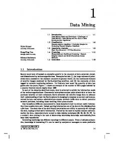
proach is flawed, in that discrimination may be the result of several joint characteristics that are not discriminatory in isolation. For instance, black cats crossing your path are typically discriminated as signs of bad luck, but no superstition is independently associated to being a cat, being black or crossing a path. In other words, the condition that describes a (minority) population that may be the object of discrimination should be stated as a conjunction of attributes values: pregnant women, minority ethnicity in disadvantaged neighborhoods, senior people in weak economic conditions, and so on. Coherently, we qualify as potentially discriminatory (PD) some selected itemsets, not necessarily single items nor whole attributes. Two consequences of this approach should be considered. First, single PD items or attributes are just a particular case in this more general setting. Second, PD itemsets are closed under intersection: the conjunction of two PD itemsets is a PD itemset as well, coherently with the intuition that the intersection of two disadvantaged minorities is a, possibly empty, smaller (even more disadvantaged) minority as well. In our approach, we assume that the analyst interested in studying discrimination compiles a list of PD itemsets with reference to attribute and attribute values that are present either in the data, or in his/her background knowledge, or in both. Discrimination has been identified in law and social study literature as either direct or indirect (sometimes called systematic). Direct discrimination consists of rules or procedures that explicitly impose “disproportionate burdens” on minority or disadvantaged groups. Indirect discrimination consists of rules or procedures that, while not explicitly mentioning discriminatory attributes, intentionally or not impose the same disproportionate burdens. Direct discrimination is modelled through potentially discriminatory rules, which are classification rules A, B → C that contain potentially discriminatory itemsets A in their premises. We show in Sect. 4.1 that there is always a unique split of the premise into a PD part and a non PD part. A PD rule does not necessarily provide evidence of discriminatory actions. In order to measure the “disproportionate burdens” that a rule imposes, the notion of α-protection is introduced as a measure of the discrimination power of a PD classification rule. The idea is to define such a measure as the relative gain in confidence of the rule due to the presence of the discriminatory itemsets. The α parameter is the key for tuning the desired level of protection against discrimination. PD classification rules are extracted (see Fig. 1 left) from a dataset containing discriminatory itemsets. This is the case, for instance, when: • internal auditors or regulation authorities want to identify discriminatory rules to the purpose of discovering malpractices that emerge from the historical transactions; they collect the dataset of past transactions and enrich it with potentially discriminatory itemsets in order to extract discriminatory PD rules; • data miners want to extract models from a dataset that contains potentially discriminatory attributes that are essential for the purpose of classification, such as in the case of gender, age, and job type. Using these attributes for building classifiers is perfectly legal: it is their use in discriminatory decisions that may be illegal! Thus, data miners must remove from the set of extracted PD rules the discriminatory ones;
Discriminatory PD Rules
A, B
Discriminatory PD Rules
C
C
PD Rules
Dataset with discriminatory items
C
Check indirect discrimination through an inference model
Check direct discrimination
A, B
A, B
D, B
C
PND Rules
Background Rules
Dataset without discriminatory items
Background Knowledge
A, B D, B
D A
Figure 1: Modelling the process of direct (left) and indirect (right) discrimination control. • consumer advisor councils or regulation authorities want to identify certain expected discriminatory PD rules to the purpose of checking that the results of specific positive discrimination policies – or affirmative actions, that tend to favor some disadvantaged categories – actually emerge from the historical transactions. Concerning indirect discrimination, we consider rules D, B → C that are potentially non-discriminatory (PND), i.e., that do not contain PD itemsets. They are extracted (see Fig. 1 right) from a dataset which may or may NOT contain PD itemsets. While apparently safe, PND rules may lead to discrimination as well. As an example, assume that the PND rule “rarely give credit to persons from neighborhood 10451 from NYC” is extracted. This may be or may be not a redlining rule. In order to unveil its nature, we have to rely on additional background knowledge. If we know that in NYC people from neighborhood 10451 are in majority black race, then using the rule above is like using the rule “rarely give credit to black-race persons from neighborhood 10451 of NYC”, which is definitely discriminatory. This use case resembles the situation described in privacy-preserving data mining [2, 15], where an anonymized dataset coupled with external knowledge might allow for the inference of the identity of individuals. In our framework, we assume that background knowledge takes the form of association rules relating a non-discriminatory itemset D to a discriminatory itemset A within the context B. Examples of background knowledge include the one originating from publicly available data (e.g., census data), from privately owned data (e.g., market surveys) or from experts or common sense (e.g., expert rules about customer behavior). Again, internal auditors, regulation authorities, consumer advisory councils, and data miners are interested for their own purposes in checking indirect discrimination by identifying PND rules that are to a certain extent equivalent to discriminatory PD rules. In order to model such a situation, we consider an inference model, i.e., a strategy that an analyst, provided with background knowledge, can pursue in order to unveil discriminatory PD rules starting from PND ones. As an example of the overall processes shown in Fig. 1, consider the rules: a. city=NYC ==> class=bad -- conf:(0.25)
b. race=black, city=NYC ==> class=bad -- conf:(0.75)
Rule (a) can be translated into the statement “people who live in NYC are assigned the bad credit class” 25% of times. Rule (b) concentrates on “black people from NYC”. In this case, the additional (discriminatory) item in the premise increases the confidence of the rule up to 75%! α-protection is intended to detect rules where such an increase is lower than a fixed threshold α. In direct discrimination, rules such as (a) and (b) above are extracted from the dataset and then α-protection can be easily checked (see Fig. 1 left). For instance, if the threshold for acceptable α-protection has been fixed to 3, rule (b) is classified as discriminatory. Tackling indirect discrimination is more challenging. Continuing the example, consider the classification rule: c. neighborhood=10451, city=NYC ==> class=bad -- conf:(0.95) extracted from a dataset where potentially discriminatory itemsets, such as race=black, are NOT present (see Fig. 1 right). Taken in isolation, rule (c) cannot be considered discriminatory or not. Assume now to know that people from neighborhood 10451 are in majority black, i.e., the following association rule holds: d. neighborhood=10451, city=NYC ==> race=black -- conf:(0.80) Despite rule (c) contains no discriminatory item, it leads to the (discriminatory) decision of denying credit to a minority sub-group (black people) which has been “redlined” by their ZIP code. In other words, the PD rule: e. race=black, neighborhood=10451, city=NYC ==> class=bad can be inferred from (c) and (d), together with a lower bound of 94% for its confidence. Such a lower bound shows a disproportionate burden (94% / 25%, i.e., 3.7 times) over black people living in neighborhood 10451. We will show a formal theorem that allows us to derive the lower bound for α-protection of (e) starting from PND rules (a) and (c) and a lower bound on the confidence of the background rule (d). Clearly, the proposed inference model provides sufficient conditions for checking indirect discrimination. If the inferred lower bound is not as high as to conclude non α-protection, we cannot state that an analyst has no other means to derive the same conclusion, e.g., by using another inference model or additional background knowledge.
The German credit case study Throughout the paper, we illustrate the notions introduced by analysing the public domain German credit dataset [11], consisting of 1000 transactions representing the good/bad credit class of bank account holders. The dataset include nominal (or discretized) attributes on personal properties: checking account status, duration, savings status, property magnitude, type of housing; on past/current credits and requested credit: credit history, credit request purpose, credit request amount, installment commitment, existing credits, other parties, other payment plan; on employment status: job type, employment since, number of dependents, own telephone; and on personal attributes: personal status and gender, age, resident since, foreign worker.
3. BASIC DEFINITIONS 3.1 Association and Classification Rules We recall the notions of itemsets, association rules and classification rules from standard definitions [1, 10, 18]. Let R be a relation with attributes a1 , . . . , an . A class attribute is a fixed attribute c of the relation. An a-item is an expression a = v, where a is an attribute and v ∈ dom(a), the domain of a. We assume that dom(a) is finite for every attribute a. A c-item is called a class item. An item is any a-item. Let I be the set of all items. A transaction is a subset of I, with exactly one a-item for every attribute a. A database of transactions, denoted by D, is a set of transactions. An itemset X is a subset of I. We denote by 2I the set of all itemsets. As usual in the literature, we write X, Y for X ∪ Y. For a transaction T , we say that T verifies X if X ⊆ T . The support of an itemset X w.r.t. a nonempty transaction database D is the ratio of transactions in D verifying X: suppD (X) = |{ T ∈ D | X ⊆ T }|/|D|, where | | is the cardinality operator. An association rule is an expression X → Y, where X and Y are itemsets. X is called the premise (or the body) and Y is called the consequence (or the head) of the association rule. We say that X → Y is a classification rule if Y is a class item and X contains no class item. We refer the reader to [10, 18] for a discussion of the integration of classification and association rule mining. The support of X → Y w.r.t. D is defined as: suppD (X → Y) = suppD (X, Y). The confidence of X → Y, defined when suppD (X) > 0, is: confD (X → Y) = suppD (X, Y)/suppD (X). Support and confidence range over [0, 1]. We omit the subscripts in suppD () and confD () when clear from the context. Since the seminal paper by Agrawal and Srikant [1], a number of well explored algorithms [5] have been introduced in order to extract frequent itemsets, i.e. itemsets with a specified minimum support, and valid association rules, i.e. rules with a specified minimum confidence.
3.2 Extended Lift We introduce a key concept for our purposes. Definition 3.1. [Extended lift] Let A, B → C be an association rule such that conf (B → C) > 0. We define the extended lift of the rule with respect to B as: conf (A, B → C) . conf (B → C) We call B the context, and B → C the base-rule. Intuitively, the extended lift expresses the relative variation of confidence due to the addition of the extra itemset A in the premise of the base rule B → C. In general, the extended lift ranges over [0, ∞[. However, if association rules with a minimum support ms > 0 are considered, it ranges over [0, 1/ms]. Similarly, if association rules with base-rules with a minimum confidence mc > 0 are considered, it ranges over [0, 1/mc]. The extended lift can be traced back to the well-known measure of lift [16], defined as: lif tB (A → C) = confB (A → C)/suppB (C), when B = {T ∈ D |B ⊆ T }. When B is empty, the extended lift reduces to the standard lift.
4.
MEASURING DISCRIMINATION
4.1 Discriminatory Itemsets and Rules Our starting point consists of flagging at syntax level those itemsets which might potentially lead to discrimination in the sense explained in the introduction. A set of itemsets I ⊆ 2I is downward closed if when A1 ∈ I and A2 ∈ I then A1 , A2 ∈ I. Definition 4.1. [PD/PND itemset] A set of potentially discriminatory (PD) itemsets Id is any downward closed set. Itemsets in 2I \ Id are called potentially non-discriminatory (PND). Any itemset X can be uniquely split into a PD part A and a PND part B = X \ A by setting A to the largest subset of X that belongs to Id 1 . A simple way of defining PD itemsets is to take those that are built from a pre-defined set of items, i.e., to reduce to the case where the granularity of discrimination is at the level of items. Example 4.2. For the German credit dataset, we fix Id = 2Id , where Id is the set of the following (discriminatory) items: personal_status=female div/sep/mar (female and not single), age=(52.6-inf) (senior people), job=unemp/unskilled non res (unskilled or unemployed non-resident), and foreign_worker=yes (foreign workers). Notice that the PD part of an itemset X is now easily identifiable as X ∩ Id , and the PND part as X \ Id . It is worth noting that discriminatory items do not necessarily coincide with sensitive attributes with respect to pure privacy protection. For instance, gender is generally considered a non-sensitive attribute, whereas it can be discriminatory in many decision contexts. Moreover, note that we use the adjective potentially both for PD and PND itemsets. As we will discuss later on, also PND may unveil (indirect) discrimination. The notion of potential (non-)discrimination is now extended to classification rules. Definition 4.3. [PD/PND classification rule] A classification rule X → C is potentially discriminatory (PD) if X = A, B with A non-empty PD itemset and B PND itemset. It is potentially non-discriminatory (PND) if X is a PND itemset. It is worth noting that PD rules can be either extracted from a dataset that contain PD itemsets or inferred as shown in Fig. 1 right. PND rules can be extracted from a dataset which may or may not contain PD itemsets. Example 4.4. Consider Ex. 4.2, and the rules: a. personal_status=female div/sep/mar savings_status=no known savings ==> class=bad b.
savings_status=no known savings ==> class=bad
(a) is a PD rule since its premise contains an item belonging to Id . On the contrary, (b) is a PND rule. Notice that (b) is the base rule of (a) if we consider as context the PND part of its premise. 1 Notice that A is univocally defined. If there were two maximal A1 6= A2 subsets belonging to Id , then A1 , A2 would belong to Id as well since Id is downward closed. But then A1 or A2 would not be maximal.
4.2
α-protection We start concentrating on PD classification rules as the potential source of discrimination. In order to capture the idea of when a PD rule may lead to discrimination, we introduce the key concept of α-protective classification rules. Definition 4.5. [α-protection] Let c = A, B → C be a PD classification rule, where A is a PD and B is a PND itemset, and let: γ = conf (A, B → C)
δ = conf (B → C) > 0.
For a given threshold α ≥ 0, we say that c is α-protective if elif t(γ, δ) < α, where: elif t(γ, δ) = γ/δ. c is called α-discriminatory if elif t(γ, δ) ≥ α. Intuitively, the definition assumes that the extended lift of c w.r.t. B is a measure of the degree of discrimination of A in the context B. α-protection states that the added (potentially discriminatory) information A increases the confidence of concluding an assertion C under the base hypothesis B only by an acceptable factor, bounded by α. Example 4.6. Consider again Ex. 4.2. Fix α = 3 and consider the classification rules: a. personal_status=female div/sep/mar savings_status=no known savings ==> class=bad -- supp:(0.013) conf:(0.27) elift:(1.52) b.
age=(52.6-inf) personal_status=female div/sep/mar purpose=used car ==> class=bad -- supp:(0.003) conf:(1) elift:(6.06)
Rule (a) can be translated as follows: if we know nothing about the savings of a person asking for credit, then assign bad credit class (or bad credit class has been assigned in past) to non-single women 52% more than the average. The support of the rule is 1.3%, its confidence 27%, and its extended lift 1.52. Hence, the rule is α-protective. Also, the confidence of the base rule: savings_status=no known savings ==> class=bad is 0.27/1.52 = 17.8%. Rule (b) states that senior non-single women that want to buy a used car are assigned the bad credit class with a probability more than 6 times higher than the average one for those that ask credit for the same purpose. The support of the rule is 0.3%, its confidence 100%, and its extended lift 6.06. Hence the rule is α-discriminatory. Finally, the confidence of the base rule purpose=used car ==> class=bad is 1/6.06 = 16.5%.
4.3 Strong α-protection When the class is binary, the concept of α-protection must be strengthened, as highlighted by the next example. Example 4.7. The following PD classification rule is extracted from the German credit dataset with minimum support of 1%:
ExtractCR() C = { class items } PDgroup = PN Dgroup = ∅ for group ≥ 0 ForEach k s.t. there exists k-frequent itemsets Fk = { k-frequent itemsets } ForEach Y ∈ Fk with Y ∩ C = 6 ∅ C = Y∩C X = Y\C s = supp(Y) s0 = supp(X) // found in Fk−1 conf = s/s0 A = largest subset of X in Id group = |X \ A| If |X| = 0 add X → C to PN D group with confidence conf Else add X → C to PD group with confidence conf EndIf EndForEach EndForEach
CheckAlphaPDCR(α) ForEach group s.t. PDgroup 6= ∅ ForEach X → C ∈ PD group A = largest subset of X in Id B = X\A γ = conf (X → C) δ = conf (B → C) // found in PN Dgroup If elif t(γ, δ) ≥ α // resp., glif t(γ, δ) ≥ α output A, B → C EndIf EndForEach EndForEach
Figure 2: Extraction of PD and PND classification rules (left) and direct checking of α-discrimination (right). a-good. personal_status=female div/sep/mar purpose=used car checking_status=no checking ==> class=good -- supp:(0.011) conf:(0.846) -- conf_base:(0.963) elift:(0.88) Rule a-good has an extended lift of 0.88. Intuitively, this means that good credit class is assigned to non-single women less than the average of people that want to buy an used car and have no checking status. As a consequence, one can deduce that the bad credit class is assigned more than the average of people in the same context, i.e. the rule: a-bad.
personal_status=female div/sep/mar purpose=used car checking_status=no checking ==> class=bad -- supp:(0.002) conf:(0.154) -- conf_base:(0.037) elift:(4.15)
It is worth noting that the confidence of rule a-bad in the example is equal to 1 minus the confidence of a-good, and the same holds for the confidence of base rules. This property holds in general for binary classes. For a binary attribute a with dom(a) = {v1 , v2 }, we write ¬(a = v1 ) for a = v2 and ¬(a = v2 ) for a = v1 . Lemma 4.8. Assume that the class attribute is binary. Let A, B → C be a classification rule, and let: γ = conf (A, B → C)
δ = conf (B → C) < 1,
We have that conf (B → ¬C) > 0 and: conf (A, B → ¬C) 1−γ = . conf (B → ¬C) 1−δ As an immediate consequence, the extraction or the inference of an α-protective rule A, B → C allows the calculation of the extended lift of the dual rule A, B → ¬C, which could be α-discriminatory. We strengthen the notion of αprotection to take into account such an implication.
Definition 4.9. [Strong α-protection] Let c = A, B → C be a PD classification rule, where A is a PD and B is a PND itemset, and let: γ = conf (A, B → C)
δ = conf (B → C) > 0.
For a given threshold α ≥ 1, we say that c is strongly αprotective if glif t(γ, δ) < α, where: � γ/δ if γ ≥ δ glif t(γ, δ) = (1 − γ)/(1 − δ) otherwise If glif t(γ, δ) ≥ α, we say that c is strongly α-discriminatory. The glif t() function ranges over [1, ∞[. If classification rules with a minimum support ms > 0 are considered, it ranges over [1, 1/ms]. Moreover, for 1 > δ > 0: glif t(γ, δ) = max{elif t(γ, δ), elif t(1 − γ, 1 − δ)}.
5. DIRECT DISCRIMINATION Let us consider the case of direct discrimination, as modelled in Fig. 1 left and with α-protection as the underlying measure of discrimination. Given a set of PD classification rules A and a threshold α, the problem of checking (strong) α-protection consists of finding the largest subset of A containing only (strong) α-protective rules. This problem is solvable by directly checking the inequality of Def. 4.5 (resp., Def. 4.9), provided that the elements of the inequality are available. We define a checking algorithm that starts from the set of frequent itemsets, namely itemsets with a given minimum support. This is the output of any of the several frequent itemset extraction algorithms available at the FIMI repository [5]. The algorithm is reported in Fig. 2. On the left hand side of the figure, the extraction of PD and PND classification rules is reported. It requires a single scan of frequent itemsets ordered by the itemset size k. For k-frequent itemsets that include a class item, a single classification rule is produced in output. The confidence of the rule can be computed by looking only at itemsets of length k −1. The rules in output are distinguished between PD and PND rules, based on the presence of discriminatory items in
1e+008
minsupp=1% 1e+007
No. of PD class. rules that are α-discriminatory
No. of PD class. rules that are α-discriminatory
1e+007
1e+006
100000
10000
1000
100
10
1e+006
100000
10000
1000
100
10
1 1
0.5 1
2
3
4
5
6
1
1.5
7
2
2.5
α
α minsup=0.5%
minsup=1.0%
minconf=0% minconf=20%
minsup=0.3%
minconf=40% minconf=60%
Figure 3: Left: distributions of α-discriminatory PD classification rules. minimum confidence for base rules.
Right: contribution of setting
1e+008
minsupp=1% No. of PD class. rules that are strongly α-discriminatory
No. of PD class. rules that are strongly α-discriminatory
minconf=80%
1e+007
1e+006
100000
10000
1000
100
10
1e+006
100000
10000
1000
100
10
1 1
1 2
4
6
8
10
1.5
12
2
2.5
3
3.5
4
4.5
5
5.5
α
α minsup=1.0%
minsup=0.5%
minsup=0.3%
minconf=0% minconf=20%
minconf=40% minconf=60%
minconf=80%
Figure 4: Left: distributions of strongly α-discriminatory PD classification rules. Right: contribution of setting minimum confidence for base rules. their premises. Moreover, the rules are grouped on the basis of the size group of the PND part of the premise. The output is a collection of PD rules PDgroup and a collection of PND rules PN Dgroup . On the right hand side of Fig. 2, the extended lift of a classification rule A, B → C ∈ PDgroup is computed from its confidence and the confidence of the base rule B → C ∈ PN Dgroup .
The German credit case study The left-hand side of Fig. 3 (resp., Fig. 4) shows the distribution of α-discriminatory PD rules (resp., strong α-discriminatory PD rules) for minimum support of 1%, 0.5% and 0.3%. The figures highlight how lower support values increase the number and the proportion of PD rules and the maximum α. Notice that, for a same minimum support, α reaches higher values in Fig. 4 than in Fig. 3, since strong α-discrimination of a rule implicitly takes into account the complementary class rule, which may have a support lower than the minimum (see e.g., (a-bad) in Ex. 4.7). We report two sample PD rules with decreasing support and increasing extended lift. a1. personal_status=female div/sep/mar employment=1 class=bad -- conf:(0.027)
Rule (dbc) states that young people in the context B of people with critical credit history, residence since 2.8 years at least, with savings at most for 100 units, and with no checkings, are assigned the bad credit scoring with a confidence of 16.7%. Rule (bc) is obtained from (dbc) by discarding the item age=(-inf-30.2] in the premise, and it has a confidence of 2.7%. As discussed in Sect. 2, without any further information, we cannot say whether rule (dbc) is discriminatory or not. Assume now to know (by some background knowledge) that in the context B above, the set of persons satisfying age=(-inf-30.2] is somewhat related to the set of persons satisfying the discriminatory item personal_status=female div/sep/mar. If the two sets were exactly the same, we could replace age=(-inf-30.2] in rule (dbc) with the discriminatory item. This would lead us to the PD classification rule: abc. personal_status=female div/sep/mar, B ==> class=bad with glif t(0.167, 0.027) = 6.19, which is considerably high. In case the two sets of persons coincide only to some extent, we can still obtain some lower bound for the glif t() of (abc). In particular, assume that young people in the context B, contrarily to the average case, are almost all nonsingle women: dba. age=(-inf-30.2], B ==> personal_status=female div/sep/mar -- conf:(0.95) Is this enough to conclude that non-single women in the context are discriminated? We cannot say that: for instance, if non-single women in the context are at 99% older than 30.2 years, the remaining 1% is involved in the decisions fired by rule (dbc), hence women in the context are not discriminated by these decisions. As a consequence, we need further information about the proportion of non-single women that are younger than 30.2 years. Assume to know that such a proportion is at least 70%, i.e. :
abd. personal_status=female div/sep/mar, B ==> age=(-inf-30.2] -- conf:(0.7) By means of the forthcoming Thm. 6.2, we can state that a lower bound for the glif t() value of (abc) is 3.19. As a consequence, the rule (abc) is at least 3.19-discriminatory, i.e., non-single women in the context are imposed by (abc) a burden of at least 3.19 times than the average of people in the context. Since the German credit dataset contains the discriminatory items, we can calculate the actual glif t() value for (abc), which turns out to be 3.37. We formalize the intuitions of this example in the next result, which derives a lower bound for α-discrimination of PD classification rules given information available in PND rules (γ, δ) and information available from background rules (β1 , β2 ). The non-trivial proof of the theorem (see [12]) relies on the inclusion-exclusion principle for boolean formulas over items, and is omitted for lack of space. Theorem 6.2. Let D, B → C be a PND classification rule, and let: γ = conf (D, B → C)
δ = conf (B → C) > 0.
Let A be a PD itemset and let β1 , β2 such that: conf (A, B → D) conf (D, B → A) Called:
f (x) = elb(x, y) =
�
≥ β1 ≥ β2 > 0.
β1 (β2 + x − 1) β2 f (x)/y 0
if f (x) > 0 otherwise
if f (x) ≥ y f (x)/y f (1 − x)/(1 − y) elseif f (1 − x) > 1 − y glb(x, y) = 1 otherwise
we have:
(i) 1 − f (1 − γ) ≥ conf (A, B → C) ≥ f (γ),. (ii) for α ≥ 0, if elb(γ, δ) ≥ α, the PD classification rule A, B → C is α-discriminatory, (iii) for α ≥ 1, if glb(γ, δ) ≥ α, the PD classification rule A, B → C is strongly α-discriminatory. 2 It is worth noting that β1 and β2 are lower bounds for the confidence values of A, B → D and D, B → A respectively. This amounts to stating that the correlation between A and D in context B within the dataset must be known only with some approximation as background knowledge. Moreover, as β1 and β2 tend to 1, the lower and upper bounds in (i) tend to γ. Also, f (γ) is monotonic w.r.t both β1 and β2 , but an increase of β1 leads to a proportional improvement of the precision of lower and upper bounds, while an increase of β2 leads to a more than proportional improvement. Example 6.3. Reconsider Ex. 6.1. We have γ = 0.167, δ = 0.027, β1 = 0.7, and β2 = 0.95. The lower bound for the glif t() value of rule abc is computed as follows. Called: 0.7 (0.95 + x − 1), 0.95 we have f (0.167) = 0.086 > 0.027, and then glb(0.833, 0.973) = f (0.167)/0.027 = 3.19. f (x) =
Recalling the redlining example, an application of Thm. 6.2 allows us to conclude that black people (race=black) are discriminated in a context (city=NYC) because almost all people living in a certain neighborhood (neighborhood=10451) are black (this is β2 ) and almost all black people live in that neighborhood (this is β1 ). In general, this is not the case, since black people live in many different neighborhoods. Moreover, in the redlining example we had to provide, as background knowledge, only the approximation β2 . However, notice that the conclusion of the example is slightly different from the one above, stating that black people who live in a certain neighborhood (race=black, neighborhood=10451) are discriminated w.r.t. people in the context (city=NYC). Such an inference can be modelled as an instance of Thm. 6.2. Example 6.4. Rules (a) and (c) from Sect. 2 a. city=NYC ==> class=bad -- conf:(0.25)
c. neighborhood=10451, city=NYC ==> class=bad -- conf:(0.95)
are instances respectively of B → C and D, B → C in Thm. 6.2, with B = city=NYC, D = neighborhood=10451 and C = class=bad. Hence, γ = 0.95 and δ = 0.25. What should be a set of PD itemsets for reasoning about redlining? Certainly, neighborhood=10451 alone cannot be considered discriminatory. However, the pair A = race=black, neighborhood=10451 might denote a possible discrimination against black people in a specific neighborhood. In general, all conjunctions of items of minority races and neighborhoods is a source of potential discrimination. This set of itemsets is downward closed, albeit not in the form of 2J for a set of items J. As background knowledge, we can now refer to census data, reporting distribution of population over the territory. So, we can easily gather statistics such as rule (d) from Sect. 2, which can be rewritten as: d. neighborhood=10451, city=NYC ==> race=black, neighborhood=10451 -- conf:(0.8) This is an instance of D, B → A in Thm. 6.2. The other expected background rule is A, B → D, which readily has confidence 100%, i.e. β1 = 1, since A contains D. So, we have not to take it into account in this redlining example, which therefore represents a simpler inference problem than the one considered in Thm. 6.2. By the conclusion of the theorem, we obtain lower bounds for the confidence and the extended lift of A, B → C, i.e., rule (e) from Sect. 2: e. race=black, neighborhood=10451, city=NYC ==> class=bad Confidence of (e) is at least 1/0.8(0.8 + 0.95 − 1) = 0.9375, and then its extended lift (w.r.t. the context city=NYC) is at least 0.9375/0.25 = 3.75. Summarizing, the classification rule (e) is at least 3.75-discriminatory or, in intuitive words, (c) is a redlining rule imposing a “disproportionate burden” (of 3.75 times than the average of NYC people) over black-race people living in neighborhood 10451. Given a set of PND classification rules PN D and a set of background rules BR, we define the absolute recall at α as the number of α-discriminatory PD rules that are inferrable by Thm. 6.2. In order to test the proposed inference model,
CheckAlphaPNDCR(α) ForEach g s.t. PN D g 6= ∅ ForEach X → C ∈ PN Dg γ = conf (X → C) generateContexts = true ForEach X → A ∈ BRg order by conf (X → A) descending β2 = conf (X → A) s = supp(X → A) (i) If β2 > 1 − γ or β2 > γ If generateContexts generateContexts = f alse V =∅ ForEach B ⊆ X // found in PN Dg0 with g 0 = |B| ≤ g δ = conf (B → C) (iii) If β2 (1 − αδ) ≥ 1 − γ or β2 (1 − α(1 − δ)) ≥ γ V = V ∪ {(B, δ)} EndIf EndForEach EndIf ForEach (B, δ) ∈ V (iii) If β2 (1 − αδ) ≥ 1 − γ or β2 (1 − α(1 − δ)) ≥ γ // found in BRg0 with g 0 = |B| ≤ g β1 = s/supp(B → A) If glb(γ, δ) ≥ α output A, B → C EndIf Else V = V \ {(B, δ)} EndIf EndForEach EndIf EndForEach EndForEach EndForEach Figure 5: Algorithm for checking indirect strong αdiscrimination. Here BRg is {X → A ∈ BR | |X| = g}. we simulate the availability of a large set of background rules under the hypothesis that the dataset contains the discriminatory items, e.g., as in the German credit case. We define: BR = {X → A | X PND, A PD, supp(X → A) ≥ ms } as the set of association rules X → A with a given minimum support. While rules of the form A, B → D seem not to be included in the background rule set, we observe that conf (A, B → D) can be obtained as supp(D, B → A)/supp(B → A), where both rules in the ratio are of the required form. Notice that the set BR contains the most precise background rules that an analyst could use, in the sense that the values for β1 and β2 in Thm. 6.2 do coincide with the confidence values they limit. Next, for each candidate rule X → C in PN D, we have to enumerate all sub-itemsets D, B ⊆ X (which are 2|X| ) such that X can be written as D, B. What we will be looking for to speed up the enumeration and checking process is some necessary conditions on the inequalities to be checked that restrict the search space. Let us start considering necessary conditions for elb(γ, δ) ≥ α. If α = 0 the expression is always true, so
No. of PD strongly α-discr. class. rules inferred from PND rules
1e+008
1e+007
1e+006
100000
10000
1000
100
10
1 1
2
3
4
5
6
α minsup=0.5%
minsup=1.0%
minsup=0.3%
Figure 6: Distribution of absolute recall. we concentrate on the case α > 0. By definition of elb(), elb(γ, δ) ≥ α > 0 happens only if f (γ) > 0 and f (γ)/δ ≥ α, which can respectively be rewritten as: (i) β2 > 1 − γ
(ii) β1 (β2 + γ − 1) ≥ αδβ2 .
Therefore, (i) is a necessary condition for elb(γ, δ) ≥ α. From (ii) and β1 ≤ 1, we can conclude elb(γ, δ) ≥ α only if β2 + γ − 1 ≥ αδβ2 , i.e.: (iii) β2 (1 − αδ) ≥ 1 − γ. Therefore, (iii) is a necessary condition for elb(γ, δ) ≥ α as well. The selectivity of conditions (i,iii) lies in the fact that checking (iii) involves no lookup at rules A, B → D; and checking (i) involves no lookup at rules B → C. Moreover, condition (iii) is monotonic w.r.t β2 , hence if we scan association rules X → A ordered by descending confidence, we can stop checking it as soon as it is false. Finally, we observe that similar necessary conditions can be derived for glb(γ, δ) ≥ α. The generate&test algorithm that incorporates the necessary conditions is shown in Fig. 5.
The German credit case study With reference to the presented test framework, Fig. 6 plots the distribution of the absolute recall of the proposed inference model by varying α and minimum support. Even for high values of α, the number of indirectly discriminatory rules is considerably high. We report below the execution times of the CheckAlphaPNDCR() procedure (on a PC with Xeon 2.4Ghz and 2Gb main memory) for rules in PN D and BR having minimum support of 1% and without/with the optimizations discussed earlier. α = 2.0 α = 1.8 α = 1.6 α = 1.4
without checks 10m21s 10m21s 10m21s 10m21s
with checks 3m12s 3m15s 3m23s 3m49s
ratio 31.0% 31.4% 32.7% 36.9%
The table shows a gain in the execution time up to 69%.
7.
RELATED WORK AND CONCLUSIONS
To the best of our knowledge, this paper is the first to address the discrimination problem in data mining models. Nevertheless, discrimination has been recognized as an issue in the tutorial [4, Slide 19] where the danger of building classifiers capable of racial discrimination in home loans has
been put forward. Technically, we measured discrimination through a generalization of lift to cope with contexts, specified as non-discriminatory itemsets. In this sense, there is a relation with the work of [13], where the notion of conditional association rules has been studied. A conditional rule A ⇔ C/B denotes a context B in which itemsets A and C are equivalent, namely where conf (A, B → C) = 1 and conf (¬A, B → ¬C) = 1. Summarizing, we have investigated how discrimination may be hidden in data mining models. Our study considered classification rules, which occur in a variety of approaches including decision trees, rule-based classifiers, and association rule-based classifiers. As the contributions of the paper, we have modelled both direct and indirect discrimination, introduced (strong) α-protection as a measure of the discriminatory power of a rule, and, as far as indirect discrimination is concerned, devised an inference model as a formal result that is able to infer discriminatory rules from apparently safe ones and some background knowledge.
8. REFERENCES [1] R. Agrawal and R. Srikant. Fast algorithms for mining association rules in large databases. In Proc. of VLDB 1994, pages 487–499. Morgan Kaufmann, 1994. [2] R. Agrawal and R. Srikant. Privacy-preserving data mining. In Proc. of SIGMOD 2000, pages 439–450. ACM, 2000. [3] G. S. Becker. The Economics of Discrimination. University of Chicago Press, 1957. [4] C. Clifton. Privacy preserving data mining: How do we mine data when we aren’t allowed to see it? Tutorial at KDD 2003. http://www.cs.purdue.edu/homes/clifton. [5] B. Goethals. Frequent Itemset Mining Implementations Repository, http://fimi.cs.helsinki.fi. [6] H. Holzer, S. Raphael, and M. Stoll. Black job applicants and the hiring officer’s race. Industrial and Labor Relations Review, 57(2):267–287, 2004. [7] D.H. Kaye and M. Aickin, editors. Statistical Methods in Discrimination Litigation. Marcel Dekker, Inc., 1992. [8] P. Kuhn. Sex discrimination in labor markets: The role of statistical evidence. The American Economic Review, 77:567–583, 1987. [9] M. LaCour-Little. Discrimination in mortgage lending: A critical review of the literature. J. of Real Estate Literature, 7:15–50, 1999. [10] B. Liu, W. Hsu, and Y. Ma. Integrating classification and association rule mining. In Proc. of KDD 1998, pages 80–86. AAAI Press, 1998. [11] D.J. Newman, S. Hettich, C.L. Blake, and C.J. Merz. UCI repository of machine learning databases, 1998. http://archive.ics.uci.edu/ml. [12] D. Pedreschi, S. Ruggieri, and F. Turini. Discrimination-aware data mining. Tech. Rep. 07-19, Dip. Inf., Univ. of Pisa, 2007. http://compass2.di.unipi.it/TR. [13] J. Rauch and M. Simunek. Mining for association rules by 4ft-Miner. In Proc. of INAP 2001, pages 285–295. Prolog Association of Japan, 2001. http://lispminer.vse.cz. [14] G. D. Squires. Racial profiling, insurance style: Insurance redlining and the uneven development of metropolitan areas. J. of Urban Affairs, 25(4):391–410, 2003. [15] L. Sweeney. Computational Disclosure Control: A Primer on Data Privacy Protection. PhD thesis, MIT, 2001. [16] P.-N. Tan, V. Kumar, and J. Srivastava. Selecting the right objective measure for association analysis. Inf. Syst., 29(4):293–313, 2004. [17] U.S. Federal Legislation. http://www.usdoj.gov. [18] X. Yin and J. Han. CPAR: Classification based on Predictive Association Rules. In Proc. of SIAM DM 2003, SIAM, 2003.