Discrimination of spatial and temporal .: .... seems desirable to collect data involving both ... four data sessions under each condition; observer C.N. was run.
Perception & Psychophysics 1977, Vol. 21 (4),357-364
Discrimination of spatial and temporal .: intervals defined by three light flashes: Effects of spacing on temporal judgments and of timing on spatial judgments C.E.COLLYER
University ojRhode Island, Kingston, Rhode Island 02881
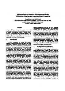
Observers were presented stimulus patterns consisting of a sequence of three laterally displaced light flashes, which defined two spatial intervals and two temporal intervals. The position and time of the second flash were varied factorially, and observers were asked to make relative judgments of either the two spatial intervals or the two temporal intervals. "Induction" effects of stimulus timing on spatial judgments and of stimulus spacing on temporal judgments were both found; however, the directionality of these effects differed between subjects. The results are inconsistent with the hypothesis, derived from previous findings, that such effects are determined primarily by a tendency toward perceiving constant velocity of apparent motion; it is proposed that the directionality of the induction effects is determined largely by the strategy adopted by the observer for combining spatial and temporal stimulus information. Three successive, laterally displaced flashes of light (or three successive, laterally displaced tactile pulses) define two successive temporal intervals and two adjoining spatial intervals. An observer may be asked to judge the relative magnitude of the two times, or of the two distances. Figure 1 illustrates the spacing and timing of three successive stimuli arrayed along one spatial dimension, and introduces some terms that will be useful in describing particular stimulus patterns. Part a of the figure shows the spatial configuration of the three stimulus positions. Part b shows the time course of their presentation. Part c is a "space-time" diagram which graphically summarizes the spatial and temporal parameters of the stimulus pattern. (The dashed lines on the diagram represent hypothetical patterns of apparent motion, which will be referred to later.) The present study employs visual stimuli and is concerned with the way in which the relative magnitudes of SI and S2 influence an observer's judgment of the relative magnitude of t l and t 2 , and vice versa. Helson (1930; Helson & King, 1931) investigated spatial judgments in the cutaneous modality. It was demonstrated that an observer's spatial judgment of the relative magnitudes of SI and S2 is strongly influenced by the relative magnitudes of t, and h. In general, if t l exceeded t 2 , then SI was judged greater than S2. This tendency in spatial judgments was termed the tau effect by Helson; this term is also used to refer to the visual analogue of the effect, which was reported by Geldreich (1934). It has also been found (Abe, 1935; Cohen et al., 1953, 1955; Price-Williams, 1954) that an observer's
temporal judgment of the relative magnitudes of t l and t 2 is strongly influenced by the relative magnitudes of SI and S2. If SI exceeded S2, then t l was judged A
B
0
1,1
C
0
~sl
;,
0
' 2 - -)t
U
A JlL-..-
_
--on.... _ __+_---rL
B , _ - -_ _ Ibl
c~
!E-!E
t}
T
llf
t2~
)!
Tlme~
IeI ~
'I
Time
Figure 1. Parameters of a dynamic stimulus pattern consisting of three successive, laterally displaced stimuli. (a) Spatial configuration of stimulus positions. (b) Time course of stimulus presentation. (c) "Space·time diagram" incorporating both spatial and temporal parameters.
358
COLLYER
to be greater than t 2 • This tendency in temporal judgments was termed the kappa effect by Cohen et al. (1953). The effect of timing on spatial judgments seems to be a distortion in the apparent relative magnitudes of s. and S2' making them more similar to the relative magnitudes of t, and t 2 • Conversely, the effect of spacing on temporal judgments seems to be a temporal distortion in the direction of the relative magnitudes of s. and S2. Both effects seem consistent with the hypothesis that observers have a perceptual tendency toward equalizing the ratios t,/t 2 and s,/s2 • This hypothesis is formally equivalent to the hypothesis that observers tend to equalize the ratios s,/t, and s2/t2 , which define velocities. (It seems reasonable that the corresponding apparent velocities are monotonic increasing functions of these ratios.) A graphic representation of this hypothesis is given in Figure 1c. The arrow represents a hypothetical perceptual tendency to distort the spatial and temporal coordinates of, in this example, the second stimulus, in a way that decreases the difference between s,/t, and s2/t2 • A version of this "constant velocity hypothesis" is implied by Cohen et al. (1955) in their discussion of the kappa effect; in a recent paper (Collyer,1976),t it was shown that such a hypothesis is consistent with the directionality of four dynamic perceptual phenomena, including the tau and kappa effects. One other of these phenomena, the induced asynchrony effect, will be briefly described. A dynamic stimulus pattern consisting of four lights arrayed horizontally is represented in Figure 2. Two initially illuminated lights, A and B, are extinguished at different times, followed after a brief dark interval by the simultaneous onsets of lights C and D. C and D are positioned at distances s, and S2, respectively, from A and B, and, in this simple case, s. = S2. In the diagram, B is extinguished before A; under these conditions, an observer would tend to judge the onset at D to occur before the onset at C, as indicated by the arrow pointing leftward. This tendency is termed the induced asynchrony effect (IAE). In general, the onset of that second stimulus (C or D), which is closer in space to the initially extinguished stimulus (A or B), will tend to be judged earlier. The dashed lines in Figure 2 represent hypothetical patterns of apparent motion between A and C and between Band D. The velocities of these apparent motions, if this aspect of perception were veridical, would be given by v, = s,/t, and V2 = s2 / h , respectively, with v. > V2 because t, < h. However, the existence of the IAE suggests that, phenomenally, t 2 is decreased relative to t, by the apparent precedence of the onset of stimulus D. Hence, the IAE might be construed as a tendency to distort V2 in the
At .........- - - -...." s1
C .J,
'"
"-",--_
.,
u ., '" Q.
Ti-me
Figure 2. Space-time diagram representing the induced asynchrony effect. The arrow signifies an observer's tendency to judge the onset of Stimulus D to precede the onset of C if the offset of Stimulus B precedes the offset of A.
direction of equality with v.. It is in this sense that the IAE, like the tau and kappa effects, appears consistent with a "constant-velocity hypothesis." It is intriguing that several phenomena should display properties which appear consistent with a general hypothesis. However, there are two important considerations which prevent us from making a strong case for the unity of these phenomena. First, as Figure 1c suggests, distortions of both space and time should occur when both the timing and the spacing of three stimuli are "uneven." However, it has not yet been shown that both distortions, tau and kappa, can be obtained using the same set ofstimulus patterns and varying only the observer's task (temporal or spatial judgment). Such a demonstration would require relatively small, confusable differences between both s. and S2 and between t, and t 2 , because, while each difference would, in one task, be a value of the "inducing" variable, in the other task it would be the quantity being judged. In order to obtain robust distortions, however, previous investigators have employed large differences on the "inducing" dimension in each task. The constantvelocity hypothesis requires that qualitatively similar, if attenuated, distortions should be observed when the inducing differences are small. A second important consideration is the difference among previous studies in the duration of the interval within which the manipulated stimulus events occur. Much of Cohen's experimental work on the kappa effect (e.g., Cohen, 1967; Cohen et al., 1953) has been done with T = 1.5 sec (see Figure 1). Higher values have also been used. Helson and King (1931) employed values of T ranging from 600 to 900 msec. In the experiments on the IAE (Collyer, 1976), however, the maximum time interval between either offset and either onset was only 150 msec; this
SPACING AND TIMING
was designed to eliminate the possibility of multiple eye fixations, which exists in the previous studies. Thus, in different studies, the time interval within which the information-carrying events in a stimulus pattern occur varies considerably. To evaluate the generality of the constant-velocity hypothesis, it seems desirable to collect data involving both temporal and spatial judgments while holding the value of T constant; furthermore, it is appropriate to keep the value of T small enough to allow the observer only one fixation.
s
o )
o
EXPERIMENT 1 This experiment employed stimulus patterns consisting of three laterally displaced lights which were illuminated briefly and in succession from left to right on each trial (as in Figure 1). The timing and positions of the peripheral lights never varied; however, the center light could be presented in one of three positions, and at one of three times, on each trial. Thus there was a total of nine stimulus patterns. The object of the experiment was to vary the question asked of the subject-sometimes he judged the relative timing of the center light, and sometimes its relative spacing-and to discover how the judgments in each case were influenced by the time and position of the center light. Method
Subjects. Three males, aged 17-20, served as paid observers. They had answered an advertisement in a local newspaper. Apparatus and Stimuli. Stimuli consisted of 6 x 4 matrices of closely spaced points on a Tektronix 602 CRT screen, and had the appearance of illuminated rectangular patches. A train of three laterally separated stimuli constituted a stimulus pattern. A DEC PDP-12 computer controlled the spacing and timing of stimuli within stimulus patterns, as well as the timing of all trial intervals and the recording of responses. The sequence of events within each trial was as follows. A fixation field, consisting of a horizontal row of 200 illuminated points and subtending about 4° visual angie, was presented for 100 msec, followed by a 500-msec dark interval. Three light flashes were then presented, as in Figure I, with S = s, + s. ~ 4°, T = t. + t. = 160 msec, and the duration of each flash equal to lO msec. The flashes were located about I ° below the fixation line. The programmed duration of the response interval was 2,000 msec; observers learned during practice to respond within this interval. Viewing distance was about 30 in. Note that the values of t. and s, are sufficient to specify a particular stimulus pattern. Design and Procedure. Three values of s, and three values of t. were combined factorially for each Observer; on each trial, the stimulus pattern presented represented one of the nine possible combinations of s. and t, values. This aspect of the design is illustrated in Figure 3. The exact values of s. and t. for each observer are given in Table 1. Different ranges of t, were chosen for each observer on the basis of preliminary data, in order to obtain roughly equal error rates. The particular combination of s. and t. employed on a given trial was randomly determined by sampling with replacement from the set of nine such combinations; the a priori probability of sampling each combination was 1/9.
359
Values of 11
T
Time
Figure 3. Space-time diagram illustrating the way in which values of t. and of s, were factorially comhined to produce nine different stimulus patterns. One of the nine combinations was sampled on each trial. There were two experimental conditions, which differed only in the judgment the observer was instructed to make. In the temporal condition, the observer's task was to report whether the second temporal interval appeared longer (an R. response) or shorter (an R. response) in duration than the first. In the spatial condition, the task was to report whether the second spatial interval appeared longer (an R. response) or shorter (an R 2 response) in extent than the first. Observers were seated in an acoustical chamber, and viewed the CRT display through a tunnel external to the window of the chamber. They were instructed to fixate "about in the middle" of the fixation line when it appeared. A fixed central fixation stimulus was avoided because it could easily serve as a reference stimulus for spatial judgments. The experimenter further instructed each observer to make spatial or temporal judgments at the beginning of each session. In both conditions, responses were made by pressing a button on the left (R.) or on the right (R 2 ) of a response panel. Daily sessions consisted of four blocks of 100 trials, separated by short rest periods. Observers L.R., M.C., and C.N. received 13, 7, and lO sessions, respectively, of preliminary experience with the experiment. Observers L.R. and M.C. were each run for four data sessions under each condition; observer C.N. was run for five data sessions under each condition. The data of main interest consisted of the proportions of R 2 responses given each Table I Values of s, in Degrees Visual Angle, and of I. in Milliseconds for Each Condition and Observer, in Experiments 1 and 2 Condition s, _ _ _ _ _ _Observer _ _ _ _ _ _ Values _ _ _of _.c.-
Values of__=_ t,
Experiment 1 Both Conditions
L.R. M.C. C.N.
1.94,2.00,2.06 1.94, 2.00, 2.06 1.94,2.00, 2.06
56,80,104 50,80,110 38.80,122
Experiment 2 Temporal Judgments Spatial Judgments
L.R. M.C. C.N.
1.75,2.00,2.25 1.75,2.00,2.25 1.75,2.00,2.25
56,80,104 50,80,110 38,80,122
L.R. M.C. C.N.
1.94,2.00,2.06 1.94,2.00, 2.06 1.94, 2.00, 2.06
20,80,140 20,80,140 20,80,140
360
COLLYER
combination of s, and t. values, for each condition and observer. The number of observations on which each such proportion is based varies, but in no case is less than 145. Sessions in Experiment I were interleaved with sessions in Experiment 2, in order to minimize differences in amount of practice between the two experiments. This was done in such a way that (1) observers performed temporal and spatial judgments on alternate days; and (2) a replication of both experiments (i.e., two sessions in Experiment I and two sessions in Experiment 2) was completed every 4 days.
Table 2 Levels of Significance Attained by a Chi-Square Statistic for Each Source of Variation in Each Observer's Response Frequency Data, in Experiment I .
Results Preliminary statistical analysis. It is of interest initially to determine whether the independent variables, s. and t.. affected the observers' judgments in each condition. For each of the six sets of data (three observers, two conditions each), the raw response frequencies conditional on each combination of s. and t. values were analyzed by a method described by Goodman (1969) for partitioning chi square in factorial experiments yielding frequency data. The results of this analysis are summarized in Table 2. The judged variable clearly influenced all three observers' judgments, in both conditions. In four of the six sets of data, the nonjudged variable had a statistically significant effect (three at p < .001 and one at p < .05). There was no significant interaction between s, and t. in any of the six cases. Temporal condition. The observed proportions, PT(R2 I s.. t.) of R 2 responses are entered in Table 3 for each stimulus pattern and observer. These proportions are plotted in Figure 4 as a function of s. for each value of t•. (The ordinate in Figures 4 through 7 is a Gaussian transformation, or probit, scale. A model which leads to this scaling will be suggested in the Discussion.)
LR ·9 ·8
-7 ·6
PS '4
'3
2
.........
-. \.
MC
Condition
Observer
Temporal
L.R. M.e. C.N.
Spatial
L.R. M.C. C.N.
*Denotes p
< .001.
Source of Variation
s,
t.
In teraction
.11 .46
* * *
.61 .89 .95
.05
.23 .76 .11
* * * *
* *
Table 3 Proportions of R 2 Responses Given Condition, Observer, and Stimulus Pattern, Experiment I Temporal Judgment Condition Observer L.R. t,
s,
2.06 2.00 1.94
56
80
.10 .14 .22
.46 .55 .64
c.s.
M.C. t, 104
50
80
t. 110
.92 .23 .43 .95 .94 .24 .48 .95 .29 .48 .97 .93 Spatial Judgment Condition
38
80
122
.19 .13 .09
.59 .52 .41
.96 .94 .93
Observer M.e. t,
L.R. t.
s,
2.06 2.00 1.94
56
80
104
50
80
110
38
80
122
.82 .56 .19
.75 .43 .19
.72
.83 .65. .50
.69 .54 .40
.54 .33 .24
.94 .79 .52
.91 .69 .33
.60 .17 .03
CN
~
.49 .22
-2
./ -)
o--a....",
I)
52 05 1= 52 . 5 1 52