optimizing of the feature transformation matrix. Section 4 contains our experimental results reported on TIMIT database. Finally, we give our conclusion in ...
Discriminative Transformations of Speech Features Based on Minimum Classification Error Behzad Zamani1, Ahmad Akbari1, Babak Nasersharif1, 2, Azarakhsh Jalalvand1,3 Audio & Speech Processing Lab, Iran University of Science & Technology, Iran 2 Computer Engineering Department, University of Guilan, Iran 3 Electronics and Information Systems (ELIS) department, Ghent University, Belgium {bzamani, akbari, nasser_s, jalalvand}@iust.ac.ir 1
Abstract: Feature extraction is an important step in pattern classification and speech recognition. Extracted features should discriminate classes from each other while being robust to the environmental conditions such as noise. For this purpose, some transformations are applied to features. In this paper, we propose a framework to improve independent feature transformations such as PCA (Principal Component Analysis), and HLDA (Heteroscedastic LDA) using the minimum classification error criterion. In this method, we modify full transformation matrices such that classification error is minimized for mapped features. We don’t reduce feature vector dimension in this mapping. The proposed methods are evaluated for continuous phoneme recognition on clean and noisy TIMIT. Experimental results show that our proposed methods improve performance of PCA, and HLDA transformation for MFCC in both clean and noisy conditions.
Keywords: Feature transformation, classification error, Speech recognition.
Minimum
1. Introduction Speech recognition systems include two main components: feature extraction and classification. The classification module is usually designed using statistical approach. A well-known classification method for speech recognition is Hidden Markov Models (HMMs). The HMM parameters are trained automatically using a training data set. A conventional training algorithm is the expectation maximization algorithm using the ML criterion. This algorithm only maximizes likelihood of each individual class. It is not chosen to discriminate between classes. Thus, discriminative training methods such as minimum classification error (MCE) [1] and maximum mutual information (MMI) [2] have been proposed. In the feature extraction module, the useful discriminative information is extracted from speech signal such that the HMM classifier can recognize different speech units including phones, tri-phones, syllables or words. The most widely used and successful speech features are Mel-frequency cepstral coefficients (MFCC). However, MFCC are not optimal for
discriminating of speech units. Their performance degrades in the presence of additive noise. Hence, several methods have been suggested for extracting more discriminative and robust features [3][4]. Linear Discriminant Analysis (LDA) based transformation is one of these approaches which transform the standard MFCCs into more discriminative features [4]. LDA transformation and its family such as Heteroscedastic LDA (HLDA) [5] and kernel LDA (KLDA) [6] can be used instead of DCT or along with DCT in MFCC extraction process [7]. Transformations like LDA and Principal Component Analysis (PCA) project the original feature vectors into a new feature space through a linear transformation matrix. They optimize transformation matrix with different goals. PCA optimizes the transformation matrix by finding the largest variations in the original feature space. On the other hand, LDA maximizes ratio of between-class variation and within-class variation when projecting the features into a subspace. The drawback of these transformations is that their optimization criteria are different from the classifier’s minimum classification error criterion [8], and can potentially corrupt the classifier performance. There are several methods to overcome this drawback. In some approaches, feature extraction and classification are conducted jointly based on a consistent criterion [4]. Minimum Classification Error (MCE) training method is an example of such methods. In this paper, we propose a framework to improve feature transformation matrices (such as PCA and HLDA) using the MCE criterion. The framework provides a full transformation matrix for mapping features. Mapping is performed without any feature dimension reduction. The rest of this paper is organized as follows. Section 2 includes a brief introduction of the MCE method. Section 3 explains our proposed framework for
optimizing of the feature transformation matrix. Section 4 contains our experimental results reported on TIMIT database. Finally, we give our conclusion in Section 5. 2. Minimum Classification Error Minimum classification error is a well-known discriminative method used for both feature transformation [9] and classifier training [1]. When the MCE method is used in training of the HMM, the parameters are adjusted to reduce the total classification error [1]. In the MCE training method, the objective function to find the HMM parameters is modeled first using a continuous function. Then, minimum of the function is found using a gradient-search method such as gradient probabilistic descent (GPD) technique [1]. However, the gradient search approaches often get trapped in local optima. A genetic-based MCE algorithm is proposed in [10] to overcome this problem. The main idea behind the MCE algorithm is to optimize an empirical error rate on the training set to improve the overall recognition rate. After the empirical training error rate is optimized by a classifier or recognizer, a biased estimate of the true error rate is obtained. One effective way to reduce this bias rate is to increase “margins” on the training data. It is desirable to use such large margins for achieving lower test errors, even if this may result in higher empirical errors in the training. This leads to methods such as Large-Margin MCE (LM-MCE) which adjusts the margin incrementally in the MCE training process such that a desirable balance can be achieved between the empirical error rates on the training set and the margin [11]. De La Torre used MCE for finding a feature transformation matrix that minimizes classification error [9]. After that, Wang and Paliwal modified this method for vowel recognition [8]. These methods define two cost functions. The first one based on addition (indexed Add) as in Equation (1) [9]. The second one based on division (indexed Div) as in Equation (2) [8]. dk ,Add (Onk , F ) = −gk (Onk , F ) +
1
η
⎡ 1
k
⎣
⎡ 1
d k , Div (O n k , F ) =
I
∑ ⎣⎢ I − 1 i =1, i ≠ k
log ⎢
⎦
(1) ⎤
(
)⎥
exp g i (O n k , F )η ⎥
η g k (O n k , F )
)
(
)
⎛
T
⎝
t =1
⎞
(
)⎠
T
T
t =1
t =1
(
logπq(i0 ) + ∑log aq(ti−)1qt + ∑logbq(ti ) onk ,t
)
Onk =W × X nk
(3) where, onk is nk-th transformed observations sequence in O n k = {o n k ,1 , o n k , 2 , ..., o n k ,T }
class k shown by nk-th X
original = {x
observation ,x
, ..., x
sequence
in
,
X nk is
class
k
}
as , Q is optimal HMM state sequence shown by Q = { q 0 , q 1 , q 2 , ..., q T } that nk
n k ,1
n k ,2
n k ,T
( achieves maximum of generated likelihood for
p O n k ; λi
).
(
p O n k ,Q ; λi
)
is
onk by Hidden Markov
Model λi with optimal state sequence Q. initial state probability of the i-th HMM,
π
a
(i ) q0
(i ) q t −1 q t
is the is the
probability of making a transition from state q t − 1 to
(
) is generated
onk ,t
in the j-th state of
state q t for the i-th HMM and b (j i ) o n , t k probability for observing vector
the i-th HMM. W is transformation matrix to be determined using MCE method. In the MCE methods, our object is to minimize the misclassification measures (1) and (2). Thus, we define a cost function that maps the misclassification measure between zero and one. For this purpose, we select sigmoid function as the cost function [8] [12]: 1 l k (Onk , F ) = 1 + exp ( −α d k (Onk , F ) ) (4) Where, d k (on , F ) is as in (1) and (2), and α is a tuning k parameter greater than one. Obviously, when d k , Add (onk , F ) is smaller than zero in equation (1), implying an accurate classification, l k (on , F ) will be k close to zero indicating no loss. A positive d k , Add (on , F ) k
⎤
I
∑ exp( gi (On , F)η)⎥⎥ ⎢ I −1i =1,i ≠k
log ⎢
(
g i Onk , F = log p Onk ,Q ; λi = log ⎜πq(i0 ) ∏aq(ti−)1qt bq(ti ) onk ,t ⎟ =
⎦
(2) where, F stands for the feature extraction parameters, I is the number of classes, η is cluster weighting which is tuned empirically. Η is a positive number represented in [1]. Η is a small fractional value that is necessary due to the very small log probabilities. g i (on , F ) is generated k
logarithm likelihood for observation Onk defined as:
represents a penalty in the form of the classification error. For an observation, onk , the total classification error is computed by [8,9]:
L =
I
Nk
∑ ∑ l k (O n k =1 n =1
k
,F )
(5) We want to find the transformation matrix W which minimizes total classification error, L. The transformation matrix can now be computed using the gradient descent method for function L as represented in [9]: k
w n ,m ,iter = w n ,m ,iter −1 − β
∂L ∂w n
Or in a matrix form as,
(6)
W iter = W iter −1 − β
Now, we need to compute ∂g i (on , F ) in relation (10) and
∂L
k
∂W
(7) Where, W is the transformation matrix; n and m indicate indexes of elements of W; iter denotes iteration number in gradient descent algorithm and β is the learning parameter. Equations (6) and (7) represent an iterative process. The iteration is stopped when total classification error, L, is lower than a threshold. In this paper, we use full transformation MCE matrix in relation (7). 3. Improving Feature Transformation Using MCE Method
(8) Where, cost function l k (on , F ) is defined as a sigmoid k function of an error measure, d k (on , F ) , as in (4). Using k relation (4), we obtain, k
(
= α lk (On , F ) 1 − lk (On , F ) k
k
)
k
k
∂W
=−
k
∂W
(9)
+
⎧ ⎫ ⎪⎪ exp g i (O n , F )η ∂g i (O n , F ) ⎪ ⎪ k k × ⎬ ∑⎨ I W ∂ i =1, i ≠ k ⎪ ⎪ exp g j (O n , F )η ∑ k ⎪⎩ j =1, j ≠ k ⎪⎭ (10) I
(
)
(
)
(11)
∂gk (On , F) k
∂W
−2
gk (On , F)log k
π q( i )
Onk = W × X nk ). to
onk and so W (because
a q( it −)1 q t
and
0
are constant respect
Onk and so W. ∂W
t =1
T
b
(k ) j
(o )
−∑ δ (qt − j )∑ γ (jmk ) on , t ⎡ C (jmk ) t =1
k
m =1
⎡ 1 I ⎤ exp( gi (On , F)η) ⎢⎣I −1i =∑ ⎥⎦ k 1,i ≠k
nk , t
∂W
nk , t
( ) ⎣(
M
(o ) =
∂b j
(k )
1
T
= ∑ δ (qt − j )
) (o −1
nk , t
)
− μ (jmk ) xtT ⎤
⎦
(12) Where, k = 1, 2, ..., I denotes the I competing models; j
is the current state index; M is number of mixtures; δ (.) is Kronecker delta function; qt is HMM state at time t; xt
onk ,t
is the t-th original feature vector; transformed feature vector using number of observations and
b
probability for observing vector the k-th HMM, defined as: k ,t
⎝
onk ,t = wxnk ,t
(o )
(k ) j
nk , t
on
k
,t
indicates ; T is the
is generated
in the j-th state of
M
b(jk ) ⎛⎜ on
∑
⎞= c(k )b(k ) ⎛⎜ o ⎞⎟ = ⎟ ⎠ m =1 jm jm ⎝ nk ,t ⎠
(k ) 1 M c jm exp ⎛⎜ − 1 ⎛ o − μ (k ) ⎞T C (k ) ⎜ n ∑ jm ⎟ jm 1 ⎜ 2 ⎝ nk ,t ⎠ (2π ) 2 m=1 C (k ) 2 ⎝
( )
−1
⎛o ⎜ nk ,t ⎝
⎞
− μ (jmk ) ⎞⎟ ⎟ ⎠⎟ ⎠
Where, o n k ,t : Observation vector for frame t
μ jm
(k )
: Mean vector of the m-th Gaussian mixture in the state j of the k-th HMM n: dimensionality of observation vector (k ) C jm : Covariance matrix of the m-th Gaussian mixture in state j of the k-th HMM
c (jmk )
: Weight of the m-th Gaussian mixture in the state j (k ) γ jm o n ,t is defined as: of the k-th HMM and
(
⎧ ⎫ I ∂dk ,Div (On , F) −1 −1 ⎪⎪ exp( gi (Onk , F)η) ∂gi (Onk , F)⎪⎪ k =η gk (On , F) ∑ ⎨ I × ⎬ k ∂W ∂W ⎪ i =1,i ≠k ⎪ ∑ exp( g j (On , F)η) k ⎪⎩j =1, j ≠k ⎪⎭ −
is a function of
jm
we use relations (1) and (2). After computing derivations of relations (1) and (2), we can write: ∂g k (O n , F )
)
(13)
To compute the second term ∂d k (onk , F ) in relation (8), ∂W ∂d k , Add (O n , F )
(
b (j i ) o n k , t
k
∂l (O n , F ) ∂l (O n , F ) ∂d (O n , F ) k k k k k = k ∂W ∂d (O n , F ) ∂W k k
∂d k (On , F )
relation (3) with respect to W. The derivation result can be written as relation (12). In relation (3), term
∂g k (On , F )
One of the drawbacks of the LDA and PCA transformations is that their optimization criteria are different from the minimum classification error criteria of the classifier which may distort the classifier performance. We propose a framework here to optimize such matrices using the MCE criteria. Suppose that the transformation matrix W transforms the original n dimensional feature vector x into a new n dimensional vector y. In fact, elements of transformation matrix W are the parameters set of the feature extraction module. We want to compute a feature transformation matrix W which minimizes a cost function of classification error. For this purpose, we compute the derivative of relation (4) with respect to W [7]:
∂ l k ( On , F )
∂W (11). Since, we can obtain ∂g i (onk , F ) by differentiating of ∂W
(
γ jm o n (k )
1 2
η
k
,t
)=
(14)
(k )
(o ) (o )
(k )
c jm b jm (k )
bj
n k ,t
n k ,t
k
)
Where,
(k ) bjm (onk ,t )
is generated probability by m-th
on
,t
Gaussian mixture for observing vector k in the state j of the k-th HMM. By inserting (13) and (14) in (12) and then by inserting (12) in each of equations (10) and (11), we can compute ∂d k (on , F ) . Then, replacing the computed k
∂W
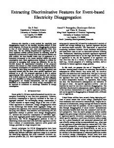
derivatives in (8) and (9) and in (7), we compute the transformation matrix. In this paper, we use HLDA and PCA transformation matrices as W, and then, optimize the feature transformation matrix W using the formula in (7). The proposed method is different from the method proposed in [8]. Fig. 1 shows this difference. Our method can be represented as minimizing classification error in a mapped space that provides optimized mapping matrix. It provides the MCE matrix for a mapped space and so mapped features, while the other proposed method finds the MCE matrix for the original space and so original features. It should be noticed that after obtaining our improved transformation matrix, we apply it to the original features in both test and train phases. In addition, Wang and Paliwal used distance classifier to calculate total classification error, while we used likelihoods of HMM.
(a) Wang and Paliwal method [8]
task. We use 39 phone classes as in [13]. We report phoneme error recognition rate (PER) on TIMIT database. In all experiments, we use 39-dimension feature vectors consisting of energy, 12 MFCCs and their first and second order derivatives. The features were normalized to have mean zero and standard deviation one over TIMIT training set. TABLE I. Explanation of Algorithm names (*: proposed methods) MCE-D
MCE Algorithm using relation (2 )
MCE-A
MCE Algorithm using relation (1)
PCA
Principal component analysis
HLDA
Heteroscedastic LDA [5]
PCAMCE-A-Init
PCA matrix as initial value for MCE-A
PCAMCE-D-Init
PCA matrix as initial value for MCE-D
*PCAMCE-A-Imp *PCAMCE-D-Imp
Improved feature transformation using PCA and MCE-A method Improved feature transformation using PCA and MCE-D
HLDAMCE-A-Init
HLDA matrix as initial value for MCE-A
HLDAMCE-D-Init
HLDA matrix as initial value for MCE-D
*HLDAMCE-A-Imp *HLDAMCE-D-Imp
Improved feature transformation using HLDA and MCE-A Improved feature transformation method
We don’t reduce features vector dimension in our methods. In addition, we use HMMs with 3 states and 16 Gaussian mixtures per state. We use TIMIT train set for training HMMs and utilize its test set for recognition experiments. For showing performance of our methods in noisy conditions, we added noise to TIMIT test set. We selected three noises from NOISEX92 database: white, pink and factory1. Then, we added these noises to all of TIMIT test set sentences with different SNR values of 0, 5, 10, 15 and 20 dB. HMMs are trained using clean training set of TIMIT database. MCE parameters, α, β and η, for TIMIT, have been set to 0.1, 0.1 and 0.005, respectively. TABLE II. PER on clean TIMIT noisy and clean test sets Clean
(b) The proposed method Fig. 1. Differences between the proposed method and Wang and Paliwal method
4. Improving Feature Transformation Using MCE Method We have introduced our abbreviations for the names of methods in Table. I. “Imp” in the name indicates that this method computes an improved transformation matrix on mapped features, while “Init” indicates that it computes transformation matrix using the original (initial) features. To evaluate the proposed methods, we have performed several experiments on the TIMIT phone recognition
Noisy (Average on 0-20dB and 3 noise types)
MFCC
28.31
52.08
MCE-A
28.17
52.03
MCE-D
28.24
52.01
PCA
29.82
52.49
PCAMCE-D-Imp
28.21
51.94
PCAMCE-A-Imp
28.19
51.83
PCAMCE-D-Init
28.75
52.32
PCAMCE-A-Init
31.01
54.01
HLDA
29.61
51.23
HLDAMCE-D- Imp
28.17
51.21
HLDAMCE-A- Imp
28.07
51.12
HLDAMCE-D-Init
28.78
52.30
HLDAMCE-A-Init
29.71
51.93
In Table II, we report phone error recognition results for noisy and clean test set. Results on noisy test set are averaged on all three noise types and SNR values 0 to 20 dB. As shown in the table, the proposed framework
improves the performance of PCA and HLDA transformation in both noisy and clean conditions. In addition, improved transformations also do better than Wang’s methods (named by “init”). Improved HLDA transformation has the best results among other methods. 5. Conclusions In this paper, we proposed a framework for improving PCA and HLDA feature transformation methods based on the minimum classification error criterion. In our approach, we change full transformation matrices such that the classification error is minimized for mapped features. This can also be considered as minimizing the classification error in a mapped space generated by improved mapping matrices. In our method, the dimension of original and the mapped spaces are the same. These optimized matrices improve PCA and HLDA performance on noisy and clean TIMIT database for continuous phoneme recognition. References [1] B. H. Juang, W.Chou and C.H.Lee, “Minimum classification error rate methods for speech recognition”, IEEE Transaction on Speech and Audio Processing, Vol. 5, No. 3, pp. 257-265, 1997. [2] V. Valtchev, Discriminative methods in HMM-based speech recognition, P.h.D thesis, Cambridge University, Cambridge, UK, 1995. [3] B. Nasersharif and A. Akbari, “SNR-dependent compression of enhanced Mel sub-band energies for compensation of noise effects on MFCC features”, Pattern Recognition Letters, Vol. 28, No. 11, pp. 1320-1326, 2007.
[4] P. Somervuo, “Experiments With Linear And Nonlinear Feature Transformations In HMM Based Phone Recognition”, IEEE International conference on Acoustics, Speech and Signal Processing, Vol. 1, pp. 52-55, 2003. [5] M. Loog and R. P. W. Duin, “Linear Dimensionality Reduction via a Heteroscedastic Extension of LDA: The Chernoff Criterion”, IEEE Transactions on Pattern Analysis and Machine Intelligence, Vol. 26, No. 6, pp.732-739, 2004. [6] A. Kocsor and L.Toth, “Kernel-Based Feature Extraction with a Speech Technology Application”, IEEE Transaction on Signal Processing, Vol. 52, No. 8, pp. 2250-2263. 2004. [7] X. B.Li , J. Y.Li, and R. H. Wang, “Dimensionality reduction using MCE-optimized LDA transformation”, IEEE International conference on Acoustics, Speech and Signal Processing, pp. 137140, 2004.. [8] X.Wang, and K. K. Paliwal, “Feature extraction and dimensionality reduction algorithms and their applications in vowel recognition”, Pattern Recognition, Vol. 36, pp. 2429-2439, 2003. [9] A. De La Torre, A. M Peinado, A. J. Rubio, V. E. Sanchez and J. E. Diaz, , “An Application of Minimum Classification Error to Feature Space Transformation for Speech Recognition”, Speech Communication, No. 20, pp. 273-290, 1996. [10] S. Kwong and Q. H. He, ”Minimum classification Error Rate Method using Genetic Algorithms”, Signal Processing, Vol. 82, No. 5, pp. 737-748, 2002. [11] D. Yu,, L. Deng, X. He and A. Acero, “Use of incrementally regulated discriminative margins in MCE training for speech recognition”, Interspeech Conference, pp. 2418-2421, 2006. [12] N. Thakoor, J. Gao and S. Jung,”Hidden Markov Model-Based Weighted Likelihood Discriminant for 2-D Shape Classification”, IEEE Transactions on Image Processing, Vol. 16, No. 11, pp. 2707-2719, 2007. [13] K. F. Lee and H. W. Hon, "Speaker-Independent Phone Recognition Using Hidden Markov Models," IEEE Transaction on Acoustics, Speech and Signal Processing, Vol. 37, No. 11, pp. 1641-1648, 1989.