Discriminative Word Alignment via Alignment Matrix Modeling Stephan Vogel Language Technologies Institute Carnegie Mellon University Pittsburgh, PA, 15213, USA
[email protected]
Jan Niehues Institut f¨ur Theoretische Informatik Universit¨at Karlsruhe (TH) Karlsruhe, Germany
[email protected]
Abstract In this paper a new discriminative word alignment method is presented. This approach models directly the alignment matrix by a conditional random field (CRF) and so no restrictions to the alignments have to be made. Furthermore, it is easy to add features and so all available information can be used. Since the structure of the CRFs can get complex, the inference can only be done approximately and the standard algorithms had to be adapted. In addition, different methods to train the model have been developed. Using this approach the alignment quality could be improved by up to 23 percent for 3 different language pairs compared to a combination of both IBM4alignments. Furthermore the word alignment was used to generate new phrase tables. These could improve the translation quality significantly.
1
Introduction
In machine translation parallel corpora are one very important knowledge source. These corpora are often aligned at the sentence level, but to use them in the systems in most cases a word alignment is needed. Therefore, for a given source sentence f1J and a given target sentence eI1 a set of links (j, i) has to be found, which describes which source word fj is translated into which target word ei . Most SMT systems use the freely available GIZA++-Toolkit to generate the word alignment. This toolkit implements the IBM- and HMMmodels introduced in (Brown et al., 1993; Vogel et al., 1996). They have the advantage that they are
trained unsupervised and are well suited for a noisychannel approach. But it is difficult to include additional features into these models. In recent years several authors (Moore et al., 2006; Lacoste-Julien et al., 2006; Blunsom and Cohn, 2006) proposed discriminative word alignment frameworks and showed that this leads to improved alignment quality. In contrast to generative models, these models need a small amount of handaligned data. But it is easy to add features to these models, so all available knowledge sources can be used to find the best alignment. The discriminative model presented in this paper uses a conditional random field (CRF) to model the alignment matrix. By modeling the matrix no restrictions to the alignment are required and even n:m alignments can be generated. Furthermore, this makes the model symmetric, so the model will produce the same alignment no matter which language is selected as source and which as target language. In contrast, in generative models the alignment is a function where a source word aligns to at most one target word. So the alignment is asymmetric. The training of this discriminative model has to be done on hand-aligned data. Different methods were tested. First, the common maximum-likelihood approach was used. In addition to this, a method to optimize the weights directly towards a word alignment metric was developed. The paper is structured as follows: Section 2 and 3 present the model and the training. In Section 4 the model is evaluated in the word alignment task as well as in the translation task. The related work and the conclusion are given in Sections 5 and 6.
18 Proceedings of the Third Workshop on Statistical Machine Translation, pages 18–25, c Columbus, Ohio, USA, June 2008. 2008 Association for Computational Linguistics
Fc (Vc ) = (f1 (Vc ), . . . , fn (Vc )) and it can be written as:
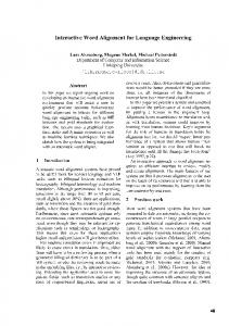
Figure 1: Alignment Example
X
Φc (Vc ) = exp(Θ ∗ Fc (Vc )) = exp(
θk ∗ fk (Vc ))
k
(1) with the weights Θ. Then the probability of an assignment of the random variables, which corresponds to a word alignment, can be expressed as: pΘ (y|e, f ) =
Y 1 Φc (Vc ) Z(e, f ) c∈V
(2)
FN
with VF N the set of all factored nodes in the graph, and the normalization factor Z(e, f ) defined as:
2
Z(e, f ) =
The Model
X Y
Φc (Vc )
(3)
Y c∈VF N
In the approach presented here the word alignment matrix is modeled by a conditional random field (CRF). A CRF is an unidirectional graphical model. It models the conditional distribution over random variables. In most applications like (Tseng et al., 2005; Sha and Pereira, 2003), a sequential model is used. But to model the alignment matrix the graphical structure of the model is more complex. The alignment matrix is described by a random variable yji for every source and target word pair (fj , ei ). These variables can have two values, 0 and 1, indicating whether these words are translations of each other or not. An example is shown in Figure 1. Gray circles represent variables with value 1, white circles stand for variables with value 0. Consequently, a word with zero fertility is indirectly modeled by setting all associated random variables to a value of 0. The structure of the CRF is described by a factored graph like it was done, for example, in (Lan et al., 2006). In this bipartite graph there are two different types of nodes. First, there are hidden nodes, which correspond to the random variables. The second type of nodes are the factored nodes c . These are not drawn in Figure 1 to keep the picture clear, but they are shown in Figure 2. They define a potential Φc on the random variables Vc they are connected to. This potential is used to describe the probability of an alignment based on the information encoded in the features. This potential is a log-linear combination of some features 19
where Y is the set of all possible alignments. In the presented model there are four different types of factored nodes corresponding to four groups of features. 2.1
Features
One main advantage of the discriminative framework is the ability to use all available knowledge sources by introducing additional features. Different features have been developed to capture different aspects of the word-alignment. The first group of features are those that depend only on the source and target words and may therefore be called local features. Consequently, the factored node corresponding to such a feature is connected to one random variable only (see Figure 2(a)). The lexical features, which represent the lexical translation probability of the words belong to this group. In our experiments the IBM4-lexica in both directions were used. Furthermore, there are source and target normalized lexical features for every lexicon. The source normalized feature, for example, is normalized in a way, that all translation probabilities of one source word to target words in the sentences sum up to one as shown in equation 4. plex (fj , ei ) (4) 1≤j≤J plex (fj , ei )
psourceN (fj , ei ) =
P
ptargetN (fj , ei ) =
P
plex (fj , ei ) (5) 1≤i≤I plex (fj , ei )
Figure 2: Different features
(a) Local features
(b) Fertility features
They compare the possible translations in one sentence similar to the rank feature used in the approach presented by Moore (2006). In addition, the following local features are used: The relative distance of the sentence positions of both words. This should help to aligned words that occur several times in the sentence. The relative edit distance between source and target word was used to improve the alignment of cognates. Furthermore a feature indicating if source and target words are identical was added to the system. This helps to align dates, numbers and names, which are quite difficult to align using only lexical features since they occur quite rarely. In some of our experiments the links of the IBM4alignments are used as an additional local feature. In the experiments this leads to 22 features. Lastly, there are indicator features for every possible combination of Parts-of-Speech(POS)-tags and for Nw high frequency words. In the experiments the 50 most frequent words were used, which lead to 2500 features and around 1440 POS-based features were used. The POS-feature can help to align words, for which the lexical features are weak. The next group of features are the fertility features. They model the probability that a word translates into one, two, three or more words, or does not have any translation at all. The corresponding factored node for a source word is connected to all I random variables representing the links to the target words, and the node for a target word is connected to all the J nodes for the links to source words (s. Figure 2(b)). In this group of features there are two different types. First, there are indicator features for the different fertilities. To reduce the complexity of the calculation this is only done up to a given maximal fertility Nf and there is an additional indicator feature for all fertilities larger than Nf . This is an 20
(c) First order features
extension of the empty word indicator feature used in other discriminative word alignment models. Furthermore, there is a real-valued feature, which can use the GIZA++ probabilities for the different fertilities. This has the advantage compared to the indicator feature that the fertility probabilities are not the same for all words. But here again, all fertilities larger than a given Nf are not considered separately. In the evaluation Nf = 3 was selected. So 12 fertility features were used in the experiments. The first-order features model the first-order dependencies between the different links. They are grouped into different directions. The factored node for the direction (s, t) is connected to the variable nodes yji and y(j+s)(i+t) . For example, the most common direction is (1, 1), which describes the situation that if the words at positions j and i are aligned, also the immediate successor words in both sentences are aligned as shown in Figure 2(c). In the default configuration the directions (1, 1), (2, 1), (1, 2) and (1, −1) are used. So this feature is able to explicitly model short jumps in the alignment, like in the directions (2, 1) and (1, 2) as well as crossing links like in the directions (1, −1). Furthermore, it can be used to improve the fertility modeling. If a word has got a fertility of two, it is often aligned to two consecutive words. Therefore, for example in the Chinese-English system the directions (1, 0) and (0, 1) were used in addition. This does not mean, that other directions in the alignment are not possible, but other jumps in the alignment do not improve the probability of the alignment. For every direction, an indicator feature that both links are active and an additional one, which also depends on the POS-pair of the first word pair is used. For a configuration with 4 directions this leads to 4 indicator features and, for example, 5760 POS-based features.
The last group of features are phrase features, which are introduced to model context dependencies. First a training corpus is aligned. Then, groups of source and target words are extracted. Words build a group, if all source words in the group are aligned to all target words. The relative frequency of this alignment is used as the feature and indicator features for 1 : 1, 1 : n, n : 1 and n : m alignments. The corresponding factored node is connected to all links that are important for this group. 2.2
potential can only have a small number of different values. This will be shown for the fertility feature node. For a more detailed description we refer to (Niehues, 2007). The message sent from a factored node to a random variable is defined in the algorithm as: mc→(j,i) (v) =
X
Φc (Vc )
(6)
Vc /v
n(j,i)0 →c (v 0 )
Y (j,i)0 ∈N (c)/(j,i)
Alignment
The structure of the described CRF is quite complex and there are many loops in the graphical structure, so the inference cannot be done exactly. For example, the random variables y(1,1) and y(1,2) as well as y(2,1) and y(2,2) are connected by the source fertility nodes of the words f1 and f2 . Furthermore the variables y(1,1) and y(2,1) as well as y(1,2) and y(2,2) are connected by the target fertility nodes. So these nodes build a loop as shown in Figure 2(b). The first order feature nodes generate loops as well. Consequently an approximation algorithm has to be used. We use the belief propagation algorithm introduced in (Pearl, 1966). In this algorithm messages consisting of a pair of two values are passed along the edges between the factored and hidden nodes for several iterations. In each iterations first messages from the hidden nodes to the connected factored nodes are sent. These messages describe the belief about the value of the hidden node calculated from the incoming messages of the other connected factored nodes. Afterwards the messages from the factored nodes to the connected hidden nodes are send. They are calculated from the potential and the other incoming messages. This algorithm is not exact in loopy graphs and it is not even possible to prove that it converges, but in (Yedidia et al., 2003) it was shown, that this algorithm leads to good results. The algorithm cannot be used directly, since the calculation of the message sent from a factored node to a random variable has an exponential runtime in the number of connected random variables. Although we limit the number of considered fertilities, the number of connected random variables can still be quite large for the fertility features and the phrase features, especially in long sentences. To reduce this complexity, we leverage the fact that the 21
where Vc is the set of random variables connected P to the factored node and Vc /v is the sum over all possible values of Vc where the random variable yji has the the value v. So the value for the message is calculated by looking at every possible combination of the other incoming messages. Then the belief for this combination is multiplied with the potential of this combination. This can be rewritten, since the potential only depends on how many links are active, not on which ones are active. mc→(j,i) (v) =
Nf X
Φc (n + v) ∗ α(n)
(7)
n=0
+ Φc (Nf + 1) ∗ α(Nf + 1) with α(n) the belief for a fertility of n of the other connected nodes and α(Nf +1) the belief for a fertility bigger than Nf with Φc (Nf + 1) the corresponding potential. The belief for a configuration of some random variables is calculated by the product over all out-going messages. So α(n) is calculated by the sum over all possible configurations that lead to a fertility of n over these products. α(n) =
X
Y
n(j,i)0 →c (v 0 )
Vc /v:|Vc |=n (j,i)0 ∈Vc /(j,i)
α(Nf + 1) =
X
Y
n(j,i)0 →c (v 0 )
Vc /v:|Vc |>Nf (j,i)0 ∈Vc /(j,i)
The values of the sums can be calculated in linear time using dynamic programming.
3
Training
The weights of the CRFs are trained using a gradient descent for a fixed number of iterations, since this approach leads already to quite good results. In the
experiments 200 iterations turned out to be a good number. The default criteria to train CRFs is to maximize the log-likelihood of the correct solution, which is given by a manually created gold standard alignment. Therefore, the feature values of the gold standard alignment and the expectation values have to be calculated for every factored node. This can be done using again the belief propagation algorithm. Often, this hand-aligned data is annotated with sure and possible links and it would be nice, if the training method could use this additional information. So we developed a method to optimize the CRFs towards the alignment error rate (AER) or the F-score with sure and possible links as introduced in (Fraser and Marcu, 2007). The advantage of the F-score is, that there is an additional parameter α, which allows to bias the metric more towards precision or more towards recall. To be able to use a gradient descent method to optimize the weights, the derivation of the word alignment metric with respect to these weights must be computed. This cannot be done for the mentioned metrics since they are not smooth functions. We follow (Gao et al., 2006; Suzuki et al., 2006) and approximate the metrics using the sigmoid function. The sigmoid function uses the probabilities for every link calculated by the belief propagation algorithm. In our experiments we compared the maximum likelihood method and the optimization towards the AER. We also tested combinations of both. The best results were obtained when the weights were first trained using the ML method and the resulting factors were used as initial values for the AER optimization. Another problem is that the POS-based features and high frequency word features have a lot more parameters than all other features and with these two types of features overfitting seems to be a bigger problem. Therefore, these features are only used in a third optimization step, in which they are optimized towards the AER, keeping all other feature weights constant. Initial results using a Gaussian prior showed no improvement.
4
Evaluation
The word alignment quality of this approach was tested on three different language pairs. On the 22
Spanish-English task the hand-aligned data provided by the TALP Research Center (Lambert et al., 2005) was used. As proposed, 100 sentences were used as development data and 400 as test data. The so called “Final Text Edition of the European Parliament Proceedings” consisting of 1.4 million sentences and this hand-aligned data was used as training corpus. The POS-tags were generated by the Brill-Tagger (Brill, 1995) and the FreeLing-Tagger (Asterias et al., 2006) for the English and the Spanish text respectively. To limit the number of different tags for Spanish we grouped them according to the first 2 characters in the tag names. A second group of experiments was done on an English-French text. The data from the 2003 NAACL shared task (Mihalcea and Pedersen, 2003) was used. This data consists of 1.1 million sentences, a validation set of 37 sentences and a test set of 447 sentences, which have been hand-aligned (Och and Ney, 2003). For the English POS-tags again the Brill Tagger was used. For the French side, the TreeTagger (Schmid, 1994) was used. Finally, to test our alignment approach with languages that differ more in structure a ChineseEnglish task was selected. As hand-aligned data 3160 sentences aligned only with sure links were used (LDC2006E93). This was split up into 2000 sentences of test data and 1160 sentences of development data. In some experiments only the first 200 sentences of the development data were used to speed up the training process. The FBIS-corpus was used as training corpus and all Chinese sentences were word segmented with the Stanford Segmenter (Tseng et al., 2005). The POS-tags for both sides were generated with the Stanford Parser (Klein and Manning, 2003). 4.1
Word alignment quality
The GIZA++-toolkit was used to train a baseline system. The models and alignment information were then used as additional knowledge source for the discriminative word alignment. For the first two tasks, all heuristics of the Pharaoh-Toolkit (Koehn et al., 2003) as well as the refined heuristic (Och and Ney, 2003) to combine both IBM4-alignments were tested and the best ones are shown in the tables. For the Chinese task only the grow-diag-final heuristic was used.
Table 1: AER-Results on EN-ES task
Name IBM4 Source-Target IBM4 Target-Source IBM4 grow-diag DWA IBM1 + IBM4 + GIZA-fert. + Link feature + POS + Phrase feature
Dev
15.26 14.23 13.28 12.26 9.21 8.84
Table 3: AER-Results on CH-EN task
Test 21.49 19.23 16.48 20.82 18.67 18.02 15.97 15.36 14.77
Name IBM4 Source-target IBM4 Target-source IBM4 Grow-diag-final DWA IBM4 - similarity + Add. directions + Big dev + Phrase feature + Phrase feature(high P.)
Table 2: AER-Results on EN-FR task
Name IBM4 Source-Target IBM4 Target-Source IBM4 intersection DWA IBM1 + HFRQ/POS + Link Feature + IBM4 + Phrase feature
Dev
5.54 3.67 3.13 3.60 3.32
Test 8.6 9.86 5.38 6.37 5.57 4.80 4.60 4.30
The results measured in AER of the discriminative word alignment for the English-Spanish task are shown in Table 1. In the experiments systems using different knowledge sources were evaluated. The first system used only the IBM1-lexica of both directions as well as the high frequent word features. Then the IBM4-lexica were used instead and in the next system the GIZA++-fertilities were added. As next knowledge source the links of both IBM4alignments were added. Furthermore, the system could be improved by using also the POS-tags. For the last system, the whole EPPS-corpus was aligned with the previous system and the phrases were extracted. Using them as additional features, the best AER of 14.77 could be reached. This is an improvement of 1.71 AER points or 10% relative to the best baseline system. Similar experiments have also been done for the English-French task. The results measured in AER are shown in Table 2. The IBM4 system uses the IBM4 lexica and links instead of the IBM1s 23
Test 44.94 37.43 35.04 30.97 30.24 27.96 27.26 27.00 26.90
and adds the GIZA++-fertilities. For the “phrase feature”-system the corpus was aligned with the “IBM4”-system and the phrases were extracted. This led to the best result with an AER of 4.30. This is 1.08 points or 20% relative improvement over the best generative system. One reason, why less knowledge sources are needed to be as good as the baseline system, may be that there are many possible links in the reference alignment and the discriminative framework can better adapt to this style. So a system using only features generated by the IBM1model could already reach an AER of 4.80. In Table 3 results for the Chinese-English alignment task are shown1 . The first system was only trained on the smaller development set and used the same knowledge source than the “IBM4”-systems in the last experiment. The system could be improved a little bit by removing the similarity feature and adding the directions (0, 1) and (1, 0) to the model. Then the same system was trained on the bigger development set. Again the parallel corpus was aligned with the discriminative word alignment system, once trained towards AER and once more towards precision, and phrases were extracted. Overall, an improvement by 8.14 points or 23% over the baseline system could be achieved. These experiments show, that every knowledge source that is available should be used. For all languages pairs additional knowledge sources lead to an improvement in the word alignment quality. A problem of the discriminative framework is, that hand-aligned data is needed for training. So the 1 For this task no results on the development task are given since different development sets were used
Table 4: Translation results for EN-ES
Name Baseline DWA
Dev 40.04 41.62
Test 47.73 48.13
Table 5: Translation results for CH-EN
Name Baseline AER F0.3 F0.7 Phrase feature AER Phrase feature F0.7
Dev 27.13 27.63 26.34 26.40 25.84 26.41
Test 22.56 23.85∗ 22.35 23.52∗ 23.42∗ 23.92∗
French-English dev set may be too small, since the best system on the development set does not correspond to the best system on the test set. And as shown in the Chinese-English task additional data can improve the alignment quality. 4.2
For the Chinese-English task some experiments were made to study the effect of different training schemes. Results are shown in Table 5. The systems used the MT’03 eval set as development data and the NIST part of the MT’06 eval set was used as test set. Scores significantly better than the baseline system are mark by a ∗ . The first three systems used a discriminative word alignment generated with the configuration as the one described as “+ big dev”system in Table 3. The first one was optimized towards AER, the other two were trained towards the F-score with an α-value of 0.3 (recall-biased) and 0.7 (precision-biased) respectively. A higher precision word alignment generates fewer alignment links, but a larger phrase table. For this task, the precision seems to be more important. So the system trained towards the AER and the F-score with an α-value of 0.7 performed better than the other systems. The phrase features gave improved performance only when optimized towards the F-score, but not when optimized towards the AER.
5
Translation quality
Since the main application of the word alignment is statistical machine translation, the aim was not only to generate better alignments measured in AER, but also to generate better translations. Therefore, the word alignment was used to extract phrases and use them then in the translation system. In all translation experiments the beam decoder as described in (Vogel, 2003) was used together with a 3-gram language model and the results are reported in the BLUE metric. For test set translations the statistical significance of the results was tested using the bootstrap technique as described in (Zhang and Vogel, 2004). The baseline system used the phrases build with the Pharaoh-Toolkit. The new word alignment was tested on the English-Spanish translation task using the TC-Star 07 development and test data. The discriminative word alignment (DWA) used the configuration denoted by +POS system in Table 1. With this configuration it took around 4 hours to align 100K sentences. But, of course, generating the alignment can be parallelized to speed up the process. As shown in Table 4 the new word alignment could generate better translations as measured in BLEU scores. 24
Comparison to other work
Several discriminative word alignment approaches have been presented in recent years. The one most similar to ours is the one presented by Blunsom and Cohn (2006). They also used CRFs, but they used two linear-chain CRFs, one for every directions. Consequently, they could find the optimal solution for each individual CRF, but they still needed the heuristics to combine both alignments. They reached an AER of 5.29 using the IBM4-alignment on the English-French task (compared to 4.30 of our approach). Lacoste-Julien et al. (2006) enriched the bipartite matching problem to model also larger fertilities and first-or der dependencies. They could reach an AER of 3.8 on the same task, but only if they also included the posteriors of the model of Liang et al. (2006). Using only the IBM4-alignment they generated an alignment with an AER of 4.5. But they did not use any POS-based features in their experiments. Finally, Moore et al. (2006) used a log-linear model for the features and performed a beam search. They could reach an AER as low as 3.7 with both types of alignment information. But they presented no results using only the IBM4-alignment features.
6
Conclusion
In this paper a new discriminative word alignment model was presented. It uses a conditional random field to model directly the alignment matrix. Therefore, the algorithms used in the CRFs had to be adapted to be able to model dependencies between many random variables. Different methods to train the model have been developed. Optimizing the Fscore allows to generate alignments focusing more on precision or on recall. For the model a multitude of features using the different knowledge sources have been developed. The experiments showed that the performance could be improved by using these additional knowledge sources. Furthermore, the use of a general machine learning framework like the CRFs enables this alignment approach to benefit from future improvements in CRFs in other areas. Experiments on 3 different language pairs have shown that word alignment quality as well as translation quality could be improved. In the translation experiments it was shown that the improvement is significant at a significance level of 5%.
References Atserias, J., B. Casas, E. Comelles, M. Gonz´alez, L. Padr´o and M. Padr´o. 2006. FreeLing 1.3: Syntactic and semantic services in an open-source NLP library. In LREC’06. Genoa, Italy. P. Blunsom and T. Cohn. 2006. Discriminative word alignment with conditional random fields. In ACL’06, pp. 65-72. Sydney, Australia. E. Brill. 1995. Transformation-based error-driven learning and natural language processing: A case study in part of speech tagging. Computational Linguistics, 21(4):543-565. P.F. Brown, S. Della Pietra, V. J. Della Pietra, R. L. Mercer. 1993. The Mathematic of Statistical Machine Translation: Parameter Estimation. Computational Linguistics, 19(2):263-311. A. Fraser, D. Marcu. 2007. Measuring Word Alignment Quality for Statistical Machine Translation Computational Linguistics, 33(3):293-303. S. Gao, W. Wu, C. Lee, T. Chua. 2006. A maximal figure-of-merit (MFoM)-learning approach to robust classifier design for text categorization. ACM Trans. Inf. Syst., 24(2):190-218. D. Klein and C.D. Manning. 2003. Fast Exact Inference with a Factored Model for Natural Language Parsing. Advances in Neural Information Processing Systems 15 (NIPS 2002), pp. 3-10.
25
P. Koehn, F. J. Och, D. Marcu. 2003. Statistical phrase-based translation. In HTL-NAACL’03, pp. 4854. Morristown, New Jersey, USA. S. Lacoste-Julien, B. Taskar, D. Klein, M. I. Jordan. 2006. Word alignment via quadratic assignment. In HTL-NAACL’06. New York, USA. P. Lambert, A. de Gispert, R. Banchs and J. b. Marino. 2005. Guidelines for Word Alignment Evaluation and Manual Alignment. Language Resources and Evaluation, pp. 267-285, Springer. X. Lan and S. Roth, D. P. Huttenlocher, M. J. Black. 2006. Efficient Belief Propagation with Learned Higher-Order Markov Random Fields. ECCV (2), Lecture Notes in Computer Science, pp. 269-282. P. Liang, B. Taskar, D. Klein. 2006. Alignment by agreement. In HTL-NAACL’06, pp. 104-110. New York, USA. R. Mihalcea, T. Pedersen. 2003. An Evaluation Exercise for Word Alignment. In HLT-NAACL 2003 Workshop, Building and Using Parallel Texts: Data Driven Machine Translation and Beyond, pp. 1-6. Edmonton,Canada. R. C. Moore, W. Yih, A. Bode. 2006. Improved discriminative bilingual word alignment. In ACL’06, pp. 513-520. Sydney, Australia. J. Niehues. 2007. Discriminative Word Alignment Models. Diplomarbeit at Universit¨at Karlsruhe(TH). F. J. Och and H. Ney. 2003. A Systematic Comparison of Various Statistical Alignment Models. Computational Linguist,29(1):19-51. J. Pearl. 1988. Probabilistic Reasoning in Intelligent Systems: Networks of Plausible Inference. H. Schmid. 1994. Probabilistic Part-of-Speech Tagging Using Decision Trees. In NEMLAP’94. Manchester, UK. F. Sha and F. Pereira. 2003. Shallow parsing with conditional random fields. In HLT-NAACL’03, pp. 134–141. Edmonton, Canada. J. Suzuki, E. McDermott, H. Isozaki. 2006. Training conditional random fields with multivariate evaluation measures In ACL’06, pp 217-224. Sydney, Australia. H. Tseng, P. Chang, G. Andrew, D. Jurafsky and C. Manning. 2005. A Conditional Random Field Word Segmenter. In SIGHAN-4. Jeju, Korea. S. Vogel, H. Ney, C. Tillmann. 1996. HMM-based word alignment in statistical translation. In COLING’96, pp. 836-841. Copenhagen, Denmark. S. Vogel. 2003. SMT Decoder Dissected: Word Reordering. In NLP-KE’03. Bejing, China. J. S. Yedidia, W. T. Freeman, Y. Weiss. 2003. Understanding belief propagation and its generalizations. Exploring artificial intelligence in the new millennium. Y. Zhang and S. Vogel. 2004. Measuring Confidence Intervals for MT Evaluation Metrics. In TMI 2004. Baltimore, MD, USA.