Log-Linear Models for Word Alignment

Log-linear Models for Word Alignment Yang Liu , Qun Liu and Shouxun Lin Institute of Computing Technology Chinese Academy of Sciences No. 6 Kexueyuan South Road, Haidian District P. O. Box 2704, Beijing, 100080, China {yliu, liuqun, sxlin}@ict.ac.cn

Abstract

data, try to describe the relationship between a bilingual sentence pair (Brown et al., 1993; Vogel and Ney, 1996). Heuristic approaches obtain word alignments by using various similarity functions between the types of the two languages (Smadja et al., 1996; Ker and Chang, 1997; Melamed, 2000). The central distinction between statistical and heuristic approaches is that statistical approaches are based on well-founded probabilistic models while heuristic ones are not. Studies reveal that statistical alignment models outperform the simple Dice coefficient (Och and Ney, 2003).

We present a framework for word alignment based on log-linear models. All knowledge sources are treated as feature functions, which depend on the source langauge sentence, the target language sentence and possible additional variables. Log-linear models allow statistical alignment models to be easily extended by incorporating syntactic information. In this paper, we use IBM Model 3 alignment probabilities, POS correspondence, and bilingual dictionary coverage as features. Our experiments show that log-linear models significantly outperform IBM translation models.

1

Introduction

Word alignment, which can be defined as an object for indicating the corresponding words in a parallel text, was first introduced as an intermediate result of statistical translation models (Brown et al., 1993). In statistical machine translation, word alignment plays a crucial role as word-aligned corpora have been found to be an excellent source of translation-related knowledge. Various methods have been proposed for finding word alignments between parallel texts. There are generally two categories of alignment approaches: statistical approaches and heuristic approaches. Statistical approaches, which depend on a set of unknown parameters that are learned from training

Finding word alignments between parallel texts, however, is still far from a trivial work due to the diversity of natural languages. For example, the alignment of words within idiomatic expressions, free translations, and missing content or function words is problematic. When two languages widely differ in word order, finding word alignments is especially hard. Therefore, it is necessary to incorporate all useful linguistic information to alleviate these problems. Tiedemann (2003) introduced a word alignment approach based on combination of association clues. Clues combination is done by disjunction of single clues, which are defined as probabilities of associations. The crucial assumption of clue combination that clues are independent of each other, however, is not always true. Och and Ney (2003) proposed Model 6, a log-linear combination of IBM translation models and HMM model. Although Model 6 yields better results than naive IBM models, it fails to include dependencies other than IBM models and HMM model. Cherry and Lin (2003) developed a

459 Proceedings of the 43rd Annual Meeting of the ACL, pages 459–466, c Ann Arbor, June 2005. 2005 Association for Computational Linguistics

statistical model to find word alignments, which allow easy integration of context-specific features. Log-linear models, which are very suitable to incorporate additional dependencies, have been successfully applied to statistical machine translation (Och and Ney, 2002). In this paper, we present a framework for word alignment based on log-linear models, allowing statistical models to be easily extended by incorporating additional syntactic dependencies. We use IBM Model 3 alignment probabilities, POS correspondence, and bilingual dictionary coverage as features. Our experiments show that log-linear models significantly outperform IBM translation models. We begin by describing log-linear models for word alignment. The design of feature functions is discussed then. Next, we present the training method and the search algorithm for log-linear models. We will follow with our experimental results and conclusion and close with a discussion of possible future directions.

2

Log-linear Models

Formally, we use following definition for alignment. Given a source (’English’) sentence e = eI1 = e1 , . . . , ei , . . . , eI and a target language (’French’) sentence f = f1J = f1 , . . . , fj , . . . , fJ . We define a link l = (i, j) to exist if ei and fj are translation (or part of a translation) of one another. We define the null link l = (i, 0) to exist if ei does not correspond to a translation for any French word in f . The null link l = (0, j) is defined similarly. An alignment a is defined as a subset of the Cartesian product of the word positions:

alignment probability is given by: P

exp[ M m=1 λm hm (a, e, f )] P r(a|e, f ) = P PM 0 a0 exp[ m=1 λm hm (a , e, f )] (2) This approach has been suggested by (Papineni et al., 1997) for a natural language understanding task and successfully applied to statistical machine translation by (Och and Ney, 2002). We obtain the following decision rule: ˆ a = argmax a

(1)

We define the alignment problem as finding the alignment a that maximizes P r(a | e, f ) given e and f. We directly model the probability P r(a | e, f ). An especially well-founded framework is maximum entropy (Berger et al., 1996). In this framework, we have a set of M feature functions hm (a, e, f ), m = 1, . . . , M . For each feature function, there exists a model parameter λm , m = 1, . . . , M . The direct 460

¾

λm hm (a, e, f )

(3)

m=1

Typically, the source language sentence e and the target sentence f are the fundamental knowledge sources for the task of finding word alignments. Linguistic data, which can be used to identify associations between lexical items are often ignored by traditional word alignment approaches. Linguistic tools such as part-of-speech taggers, parsers, namedentity recognizers have become more and more robust and available for many languages by now. It is important to make use of linguistic information to improve alignment strategies. Treated as feature functions, syntactic dependencies can be easily incorporated into log-linear models. In order to incorporate a new dependency which contains extra information other than the bilingual sentence pair, we modify Eq.2 by adding a new variable v: P

exp[ M m=1 λm hm (a, e, f , v)] P r(a|e, f , v) = P PM 0 a0 exp[ m=1 λm hm (a , e, f , v)] (4) Accordingly, we get a new decision rule: ˆ a = argmax

a ⊆ {(i, j) : i = 0, . . . , I; j = 0, . . . , J}

½X M

a

½X M

¾

λm hm (a, e, f , v)

(5)

m=1

Note that our log-linear models are different from Model 6 proposed by Och and Ney (2003), which defines the alignment problem as finding the alignment a that maximizes P r(f , a | e) given e.

3 Feature Functions In this paper, we use IBM translation Model 3 as the base feature of our log-linear models. In addition, we also make use of syntactic information such as part-of-speech tags and bilingual dictionaries.

3.1 IBM Translation Models Brown et al. (1993) proposed a series of statistical models of the translation process. IBM translation models try to model the translation probability P r(f1J |eI1 ), which describes the relationship between a source language sentence eI1 and a target language sentence f1J . In statistical alignment models P r(f1J , aJ1 |eI1 ), a ’hidden’ alignment a = aJ1 is introduced, which describes a mapping from a target position j to a source position i = aj . The relationship between the translation model and the alignment model is given by: P r(f1J |eI1 ) =

X

P r(f1J , aJ1 |eI1 )

(6)

aJ 1

Although IBM models are considered more coherent than heuristic models, they have two drawbacks. First, IBM models are restricted in a way such that each target word fj is assigned to exactly one source word eaj . A more general way is to model alignment as an arbitrary relation between source and target language positions. Second, IBM models are typically language-independent and may fail to tackle problems occurred due to specific languages. In this paper, we use Model 3 as our base feature function, which is given by 1 :

=

!

l Y m − φ0 p0 m−2φ0 p1 φ0 φi !n(φi |ei ) × φ0 i=1 m Y

t(fj |eaj )d(j|aj , l, m)

P r(fT|a, eT) =

Y

t(f Ta(j) |eTa(i) )

(8)

a

where a is an element of a, a(i) is the corresponding source position of a and a(j) is the target position. Hence, the feature function is: h(a, e, f , eT, fT) =

Y

t(f Ta(j) |eTa(i) )

(9)

a

We still distinguish between two translation directions to use POS tags Transition Model as feature functions: treating English as source language and French as target language or vice versa.

h(a, e, f ) = P r(f1J , aJ1 |eI1 )

Ã

in (Toutanova et al., 2002). They introduce additional lexicon probability for POS tags in both languages. In IBM models as well as HMM models, when one needs the model to take new information into account, one must create an extended model which can base its parameters on the previous model. In log-linear models, however, new information can be easily incorporated. We use a POS Tags Transition Model as a feature function. This feature learns POS Tags transition probabilities from held-out data (via simple counting) and then applies the learned distributions to the ranking of various word alignments. We define eT = eT1I = eT1 , . . . , eTi , . . . , eTI and fT = f T1J = f T1 , . . . , f Tj , . . . , f TJ as POS tag sequences of the sentence pair e and f . POS Tags Transition Model is formally described as:

(7)

j=1

We distinguish between two translation directions to use Model 3 as feature functions: treating English as source language and French as target language or vice versa. 3.2 POS Tags Transition Model The first linguistic information we adopt other than the source language sentence e and the target language sentence f is part-of-speech tags. The use of POS information for improving statistical alignment quality of the HMM-based model is described 1 If there is a target word which is assigned to more than one source words, h(a, e, f ) = 0.

461

3.3 Bilingual Dictionary A conventional bilingual dictionary can be considered an additional knowledge source. We could use a feature that counts how many entries of a conventional lexicon co-occur in a given alignment between the source sentence and the target sentence. Therefore, the weight for the provided conventional dictionary can be learned. The intuition is that the conventional dictionary is expected to be more reliable than the automatically trained lexicon and therefore should get a larger weight. We define a bilingual dictionary as a set of entries: D = {(e, f, conf )}. e is a source language word, f is a target langauge word, and conf is a positive real-valued number (usually, conf = 1.0) assigned

by lexicographers to evaluate the validity of the entry. Therefore, the feature function using a bilingual dictionary is: h(a, e, f , D) =

X

occur(ea(i) , fa(j) , D)

(10)

a

where (

occur(e, f, D) =

conf 0

if (e, f ) occurs in D else (11)

4 Training We use the GIS (Generalized Iterative Scaling) algorithm (Darroch and Ratcliff, 1972) to train the model parameters λM 1 of the log-linear models according to Eq. 4. By applying suitable transformations, the GIS algorithm is able to handle any type of real-valued features. In practice, We use YASMET 2 written by Franz J. Och for performing training. The renormalization needed in Eq. 4 requires a sum over a large number of possible alignments. If e has length l and f has length m, there are possible 2lm alignments between e and f (Brown et al., 1993). It is unrealistic to enumerate all possible alignments when lm is very large. Hence, we approximate this sum by sampling the space of all possible alignments by a large set of highly probable alignments. The set of considered alignments are also called n-best list of alignments. We train model parameters on a development corpus, which consists of hundreds of manually-aligned bilingual sentence pairs. Using an n-best approximation may result in the problem that the parameters trained with the GIS algorithm yield worse alignments even on the development corpus. This can happen because with the modified model scaling factors the n-best list can change significantly and can include alignments that have not been taken into account in training. To avoid this problem, we iteratively combine n-best lists to train model parameters until the resulting n-best list does not change, as suggested by Och (2002). However, as this training procedure is based on maximum likelihood criterion, there is only a loose relation to the final alignment quality on unseen bilingual texts. In practice, 2

Available at http://www.fjoch.com/YASMET.html

462

having a series of model parameters when the iteration ends, we select the model parameters that yield best alignments on the development corpus. After the bilingual sentences in the development corpus are tokenized (or segmented) and POS tagged, they can be used to train POS tags transition probabilities by counting relative frequencies: p(f T |eT ) =

NA (f T, eT ) N (eT )

Here, NA (f T, eT ) is the frequency that the POS tag f T is aligned to POS tag eT and N (eT ) is the frequency of eT in the development corpus.

5 Search We use a greedy search algorithm to search the alignment with highest probability in the space of all possible alignments. A state in this space is a partial alignment. A transition is defined as the addition of a single link to the current state. Our start state is the empty alignment, where all words in e and f are assigned to null. A terminal state is a state in which no more links can be added to increase the probability of the current alignment. Our task is to find the terminal state with the highest probability. We can compute gain, which is a heuristic function, instead of probability for efficiency. A gain is defined as follows: P

exp[ M m=1 λm hm (a ∪ l, e, f )] gain(a, l) = (12) PM exp[ m=1 λm hm (a, e, f )] where l = (i, j) is a link added to a. The greedy search algorithm for general loglinear models is formally described as follows: Input: e, f , eT, fT, and D Output: a 1. Start with a = φ. 2. Do for each l = (i, j) and l ∈ / a: Compute gain(a, l) 3. Terminate if ∀l, gain(a, l) ≤ 1. 4. Add the link ˆl with the maximal gain(a, l) to a. 5. Goto 2.

The above search algorithm, however, is not efficient for our log-linear models. It is time-consuming for each feature to figure out a probability when adding a new link, especially when the sentences are very long. For our models, gain(a, l) can be obtained in a more efficient way 3 : µ

M X

hm (a ∪ l, e, f ) gain(a, l) = λm log hm (a, e, f ) m=1

¶

(13)

Note that we restrict that h(a, e, f ) ≥ 0 for all feature functions. The original terminational condition for greedy search algorithm is: P

exp[ M m=1 λm hm (a ∪ l, e, f )] gain(a, l) = ≤ 1.0 PM exp[ m=1 λm hm (a, e, f )] That is: M X

λm [hm (a ∪ l, e, f ) − hm (a, e, f )] ≤ 0.0

3. Terminate if ∀l, gain(a, l) ≤ t. 4. Add the link ˆl with the maximal gain(a, l) to a. 5. Goto 2. The gain threshold t depends on the added link l. We remove this dependency for simplicity when using it in search algorithm by treating it as a fixed real-valued number.

6 Experimental Results We present in this section results of experiments on a parallel corpus of Chinese-English texts. Statistics for the corpus are shown in Table 1. We use a training corpus, which is used to train IBM translation models, a bilingual dictionary, a development corpus, and a test corpus.

Train

m=1

By introducing gain threshold t, we obtain a new terminational condition: µ

M X

hm (a ∪ l, e, f ) λm log hm (a, e, f ) m=1

¶

Dict Dev

≤t

where

Test

t=

M X m=1

½

λm log

µ

hm (a ∪ l, e, f ) hm (a, e, f )

¶ ¾

Sentences Words Vocabulary Entries Vocabulary Sentences Words Ave. SentLen Sentences Words Ave. SentLen

Chinese English 108 925 3 784 106 3 862 637 49 962 55 698 415 753 206 616 203 497 435 11 462 14 252 26.35 32.76 500 13 891 15 291 27.78 30.58

Table 1. Statistics of training corpus (Train), bilingual dictionary (Dict), development corpus (Dev), and test corpus (Test).

−[hm (a ∪ l, e, f ) − hm (a, e, f )] Note that we restrict h(a, e, f ) ≥ 0 for all feature functions. Gain threshold t is a real-valued number, which can be optimized on the development corpus. Therefore, we have a new search algorithm: Input: e, f , eT, fT, D and t Output: a 1. Start with a = φ. 2. Do for each l = (i, j) and l ∈ / a: Compute gain(a, l) 3

We still call the new heuristic function gain to reduce notational overhead, although the gain in Eq. 13 is not equivalent to the one in Eq. 12.

463

The Chinese sentences in both the development and test corpus are segmented and POS tagged by ICTCLAS (Zhang et al., 2003). The English sentences are tokenized by a simple tokenizer of ours and POS tagged by a rule-based tagger written by Eric Brill (Brill, 1995). We manually aligned 935 sentences, in which we selected 500 sentences as test corpus. The remaining 435 sentences are used as development corpus to train POS tags transition probabilities and to optimize the model parameters and gain threshold. Provided with human-annotated word-level alignment, we use precision, recall and AER (Och and

Model 3 E → C Model 3 C → E Intersection Union Refined Method Model 3 E → C + Model 3 C → E + POS E → C + POS C → E + Dict

1K 0.4497 0.4688 0.4588 0.4596 0.4154 0.4490 0.3970 0.3828 0.3795 0.3650

Size of Training Corpus 5K 9K 39K 0.4081 0.4009 0.3791 0.4261 0.4221 0.3856 0.4106 0.4044 0.3823 0.4210 0.4157 0.3824 0.3586 0.3499 0.3153 0.3987 0.3834 0.3639 0.3317 0.3217 0.2949 0.3182 0.3082 0.2838 0.3160 0.3032 0.2821 0.3092 0.2982 0.2738

109K 0.3745 0.3469 0.3687 0.3703 0.3068 0.3533 0.2850 0.2739 0.2726 0.2685

Table 2. Comparison of AER for results of using IBM Model 3 (GIZA++) and log-linear models. Ney, 2003) for scoring the viterbi alignments of each model against gold-standard annotated alignments: precision =

recall = AER = 1 −

|A ∩ P | |A|

|A ∩ S| |S|

|A ∩ S| + |A ∩ P | |A| + |S|

where A is the set of word pairs aligned by word alignment systems, S is the set marked in the gold standard as ”sure” and P is the set marked as ”possible” (including the ”sure” pairs). In our ChineseEnglish corpus, only one type of alignment was marked, meaning that S = P . In the following, we present the results of loglinear models for word alignment. We used GIZA++ package (Och and Ney, 2003) to train IBM translation models. The training scheme is 15 H 5 35 , which means that Model 1 are trained for five iterations, HMM model for five iterations and finally Model 3 for five iterations. Except for changing the iterations for each model, we use default configuration of GIZA++. After that, we used three types of methods for performing a symmetrization of IBM models: intersection, union, and refined methods (Och and Ney , 2003). The base feature of our log-linear models, IBM Model 3, takes the parameters generated by GIZA++ as parameters for itself. In other words, our loglinear models share GIZA++ with the same parame464

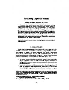
ters apart from POS transition probability table and bilingual dictionary. Table 2 compares the results of our log-linear models with IBM Model 3. From row 3 to row 7 are results obtained by IBM Model 3. From row 8 to row 12 are results obtained by log-linear models. As shown in Table 2, our log-linear models achieve better results than IBM Model 3 in all training corpus sizes. Considering Model 3 E → C of GIZA++ and ours alone, greedy search algorithm described in Section 5 yields surprisingly better alignments than hillclimbing algorithm in GIZA++. Table 3 compares the results of log-linear models with IBM Model 5. The training scheme is 15 H 5 35 45 55 . Our log-linear models still make use of the parameters generated by GIZA++. Comparing Table 3 with Table 2, we notice that our log-linear models yield slightly better alignments by employing parameters generated by the training scheme 15 H 5 35 45 55 rather than 15 H 5 35 , which can be attributed to improvement of parameters after further Model 4 and Model 5 training. For log-linear models, POS information and an additional dictionary are used, which is not the case for GIZA++/IBM models. However, treated as a method for performing symmetrization, log-linear combination alone yields better results than intersection, union, and refined methods. Figure 1 shows how gain threshold has an effect on precision, recall and AER with fixed model scaling factors. Figure 2 shows the effect of number of features

1K 0.4384 0.4564 0.4432 0.4499 0.4106 0.4372 0.3920 0.3807 0.3731 0.3612

Model 5 E → C Model 5 C → E Intersection Union Refined Method Model 3 E → C + Model 3 C → E + POS E → C + POS C → E + Dict

Size of Training Corpus 5K 9K 39K 0.3934 0.3853 0.3573 0.4067 0.3900 0.3423 0.3916 0.3798 0.3466 0.4051 0.3923 0.3516 0.3446 0.3262 0.2878 0.3873 0.3724 0.3456 0.3269 0.3167 0.2842 0.3122 0.3039 0.2732 0.3091 0.3017 0.2722 0.3046 0.2943 0.2658

109K 0.3429 0.3239 0.3267 0.3375 0.2748 0.3334 0.2727 0.2667 0.2657 0.2625

Table 3. Comparison of AER for results of using IBM Model 5 (GIZA++) and log-linear models.

Precision

M3EC M3EC + M3CE

Recall

time consumed for searching (second)

1.0

0.8

0.6

0.4

0.2

0.0

-10

-8

-6

-4

-2

0

2

4

6

8

M3EC + M3CE + POSEC + POSCE M3EC + M3CE + POSEC + POSCE + Dict

1000

800

600

400

200 -12

M3EC + M3CE + POSEC

1200

AER

1k

10

5k

9k

39k

109k

size of training corpus

gain threshold

Figure 1. Precision, recall and AER over different gain thresholds with the same model scaling factors.

and size of training corpus on search efficiency for log-linear models. Table 4 shows the resulting normalized model scaling factors. We see that adding new features also has an effect on the other model scaling factors.

7

Conclusion

We have presented a framework for word alignment based on log-linear models between parallel texts. It allows statistical models easily extended by incorporating syntactic information. We take IBM Model 3 as base feature and use syntactic information such as POS tags and bilingual dictionary. Experimental 465

Figure 2. Effect of number of features and size of training corpus on search efficiency.

λ1 λ2 λ3 λ4 λ5

MEC 1.000 -

+MCE 0.466 0.534 -

+PEC 0.291 0.312 0.397 -

+PCE 0.202 0.212 0.270 0.316 -

+Dict 0.151 0.167 0.257 0.306 0.119

Table 4. Resulting model scaling factors: λ1 : Model 3 E → C (MEC); λ2 : Model 3 C → E (MCE); λ3 : POS E → C (PEC); λ4 : POS C → E (PCE); λ5 : Dict P (normalized such that 5m=1 λm = 1). results show that log-linear models for word alignment significantly outperform IBM translation models. However, the search algorithm we proposed is

supervised, relying on a hand-aligned bilingual corpus, while the baseline approach of IBM alignments is unsupervised. Currently, we only employ three types of knowledge sources as feature functions. Syntax-based translation models, such as tree-to-string model (Yamada and Knight, 2001) and tree-to-tree model (Gildea, 2003), may be very suitable to be added into log-linear models. It is promising to optimize the model parameters directly with respect to AER as suggested in statistical machine translation (Och, 2003).

Acknowledgement This work is supported by National High Technology Research and Development Program contract ”Generally Technical Research and Basic Database Establishment of Chinese Platform” (Subject No. 2004AA114010).

I. Dan Melamed 2000. Models of translational equivalence among words. Computational Linguistics, 26(2):221-249, June. Franz J. Och and Hermann Ney. 2002. Discriminative training and maximum entropy models for statistical machine translation. In Proceedings of the 40th Annual Meeting of the Association for Computational Linguistics (ACL), pages 295-302, Philadelphia, PA, July. Franz J. Och. 2002. Statistical Machine Translation: From Single-Word Models to Alignment Templates. Ph.D. thesis, Computer Science Department, RWTH Aachen, Germany, October. Franz J. Och. 2003. Minimum error rate training in statistical machine translation. In Proceedings of the 41st Annual Meeting of the Association for Computational Linguistics (ACL), pages: 160-167, Sapporo, Japan. Franz J. Och and Hermann Ney. 2003. A systematic comparison of various statistical alignment models. Computational Linguistics, 29(1):19-51, March.

References

Kishore A. Papineni, Salim Roukos, and Todd Ward. 1997. Feature-based language understanding. In European Conf. on Speech Communication and Technology, pages 1435-1438, Rhodes, Greece, September.

Adam L. Berger, Stephen A. Della Pietra, and Vincent J. DellaPietra. 1996. A maximum entropy approach to natural language processing. Computational Linguistics, 22(1):39-72, March.

Frank Smadja, Vasileios Hatzivassiloglou, and Kathleen R. McKeown 1996. Translating collocations for bilingual lexicons: A statistical approach. Computational Linguistics, 22(1):1-38, March.

Eric Brill. 1995. Transformation-based-error-driven learning and natural language processing: A case study in part-of-speech tagging. Computational Linguistics, 21(4), December.

J¨ org Tiedemann. 2003. Combining clues for word alignment. In Proceedings of the 10th Conference of European Chapter of the ACL (EACL), Budapest, Hungary, April.

Peter F. Brown, Stephen A. Della Pietra, Vincent J. Della Pietra, and Robert. L. Mercer. 1993. The mathematics of statistical machine translation: Parameter estimation. Computational Linguistics, 19(2):263-311.

Kristina Toutanova, H. Tolga Ilhan, and Christopher D. Manning. 2003. Extensions to HMM-based statistical word alignment models. In Proceedings of Empirical Methods in Natural Langauge Processing, Philadelphia, PA.

Colin Cherry and Dekang Lin. 2003. A probability model to improve word alignment. In Proceedings of the 41st Annual Meeting of the Association for Computational Linguistics (ACL), Sapporo, Japan.

Stephan Vogel, Hermann Ney, and Christoph Tillmann. 1996. HMM-based word alignment in statistical translation. In Proceedings of the 16th Int. Conf. on Computational Linguistics, pages 836-841, Copenhagen, Denmark, August.

J. N. Darroch and D. Ratcliff. 1972. Generalized iterative scaling for log-linear models. Annals of Mathematical Statistics, 43:1470-1480. Daniel Gildea. 2003. Loosely tree-based alignment for machine translation. In Proceedings of the 41st Annual Meeting of the Association for Computational Linguistics (ACL), Sapporo, Japan. Sue J. Ker and Jason S. Chang. 1997. A class-based approach to word alignment. Computational Linguistics, 23(2):313-343, June.

466

Kenji Yamada and Kevin Knight. 2001. A syntaxbased statistical machine translation model. In Proceedings of the 39th Annual Meeting of the Association for Computational Linguistics (ACL), pages: 523-530, Toulouse, France, July. Huaping Zhang, Hongkui Yu, Deyi Xiong, and Qun Liu. 2003. HHMM-based Chinese lexical analyzer ICTCLAS. In Proceedings of the second SigHan Workshop affiliated with 41th ACL, pages: 184-187, Sapporo, Japan.