Disentangling decision models – from independence to competition
Andrei R. Teodorescu
and
Marius Usher
Tel-Aviv University
Corresponding author: Prof. Marius Usher Department of Psychology, Tel-Aviv University, Ramat-Aviv. E-mail:
[email protected] Acknowledgments: We wish to thank James L. McClelland for very stimulating input and criticism on the design of these experiments and to Konstantinos Tsetsos & Rani Moran for computational advice and constructive discussions. This research was partially supported by the Air Force Research Laboratory (FA9550-07-1-0537). Simulation codes can be found at: https://www.dropbox.com/sh/rqm5vrtr1rnzoov/zdp8THRfg0 1
Abstract A multitude of models have been proposed to account for the neural mechanism of value integration and decision making in speeded decision tasks. While most of these models account for existing data, they largely disagree on a fundamental characteristic of the choice mechanism: independent vs. different types of competitive processing. Five models, an independent race model, two types of input competition models (normalized race and Feed-Forward Inhibition [FFI]) and two types of response competition models (Max Minus Next [MMN] diffusion and Leaky Competing Accumulators [LCA]) were compared in three combined computational and experimental studies. In each study, difficulty was manipulated in a way that produced qualitatively distinct predictions from the different classes of models. When parameters were constrained by the experimental conditions to avoid mimicking, simulations demonstrated that independent models predict speedups in RT with increased difficulty, while response competition models predict the opposite. Predictions of input-competition models vary between specific models and experimental conditions. Taken together, the combined computational and empirical findings provide support for the notion that decisional processes are intrinsically competitive and that this competition is likely to kick in at a late (response) rather than early (input) processing stage.
2
Disentangling decision models – from independence to competition Decision-making is paramount in daily life, ranging from fast perceptual choices critical to survival, such as deciding whether the signal on a radar screen indicates an enemy missile or a friendly plane, to multi-dimensional, goal driven and effortconsuming decisions, such as deciding on the guilt of a defendant in a legal case. In such situations, the decision-maker is presented with samples of information and is required to decide which alternative to choose. Samples may correspond to perceptual information in the form of physical intensity values as in a sequence from a noisy visual stream (Gold & Shadlen, 2007; Glimcher, 2003), values associated with qualities of different alternatives such as consumer products, risky gambles, career choices and flat-mates (Hertwig, Barron, Weber, & Erev, 2004; Tsetsos, Usher, & Chater, 2010; Dijksterhuis, Bos, Nordgren, & van Baaren, 2006), or pieces of evidence in a legal case. The problem facing the decision maker is how to combine and weigh these samples towards a decision while at the same time limiting the amount of sampled information to determine when to terminate the process and execute a response (for further discussion, see Gold & Shadlen, 2007; Ratcliff & Smith, 2004). The mechanism that enables humans to make such decisions has been studied extensively over the last few decades both in psychology (Bogacz, Brown, Moehlis, Holmes & Cohen, 2006; Bogacz, Usher, Zhang & McClelland, 2007; Brown & Heathcote, 2008; Laming, 1968; Link & Heath, 1975; Ratcliff & Rouder, 1998; Ratcliff & Smith, 2004; Ratcliff & McKoon, 2008; Van Ravenzwaaij, Mulder, Tuerlinckx & Wagenmakers, in press; Stone, 1960; Usher & McClelland, 2001; Vickers, 1970) and in neuroscience (Albantakis, & Deco, 2009; Donner, Siegel, Fries, & Engel, 2009; Gold & Shadlen, 2007; Hanes & Schall, 1996; Mulder, Wagenmakers, Ratcliff, Boekel & Forstmann, in press; Purcell, Heitz, Cohen, Schall, Logan & Palmeri, 2010; Rorie, Gao, McClelland & Newsome, 2010; Rorie & Newsome, 2005; Wang, 2008), converging on the idea that multiple samples of information are translated to a value-scale (see Luce, 1959, and Anderson, N. H., 1971, for earlier precursors to the important role of value integration in decision-making, and Glimcher (2003) for a more recent discussion) and are accumulated, over time, towards a decision criterion. This sequential sampling principle allows the decision making mechanism to average external and internal noise over time while accounting for both response time (RT; e.g., Ratcliff & McKoon, 2008) and accuracy. The sequential sampling principle is now considered a general decision mechanism that deals with the integration of values that fluctuate over time (Gold & Shadlen, 2001, 2002; Kiani, Hanks & Shadlen, 2008; Roe, Busemeyer & Townsend, 2001; Rorie & Newsome, 2005; Sugrue, Corrado & Newsome, 2005; Usher & McClelland, 2004). In this spirit, a number of paradigms have been developed, which use noisy perceptual stimuli (such as randomly moving dots, among which a small fraction moves coherently; Shadlen & Newsome, 1996) as a proxy to more general information. While certain perceptual decisions have a quite limited temporal range 3
of integration (200-300ms) that is subject to stimulus specific properties, indicating a more idiosyncratic mechanism (Uchida, Kepecs & Mainen, 2006), other tasks implementing noisy evidence (e.g., the random-dots) show much longer integration times of up to a few seconds (Burr & Santoro, 2001; see also review in, Uchida, Kepecs & Mainen, 2006). The focus of our paper is to scrutinize the general decision mechanism responsible for such value integration and evaluation tasks by contrasting a variety of decision-making models. Indeed, a number of different mathematical models, most of which implement sequential sampling as their underlying principle, have been proposed to account for general decision behavior. Such models range from race or accumulator models (Brown & Heathcote, 2008; Smith & Vickers, 1988; VanZandt, Colonius & Proctor, 2000; Vickers, 1970), to drift-diffusion models (Link & Heath, 1975; Ratcliff, 1978; Ratcliff & Rouder, 1998; Stone, 1960), and more recent neurocomputational models introduced in an attempt to bridge the gap between previous mathematical models and the growing understanding of brain functions. A few such examples are the neural implementation of the drift diffusion model (Mazurek, Roitman, Ditterich & Shadlen, 2003; Niwa & Ditterich, 2008; Ratcliff, Hasegawa, Hasegawa, Smith & Segraves, 2007), the Leaky Competing Accumulator model (LCA; Usher & McClelland, 2001) and the attractor model (Albantakis, & Deco, 2009; Wang, 2002, 2008). The large corpus of currently available choice models can be classified according to a number of important principles that reflect distinct underlying mechanisms such as competitive vs. independent processing, relative vs. absolute decision criteria and perfect vs. leaky integration of evidence. Despite these clear processing differences, models of each type exist which are able to fit reasonably well most empirical data to date. Consequently, so far, only small quantitative differences in the goodness of fit have been found between models (Brown & Heathcote, 2008; Ratcliff & Smith, 2004; Usher & McClelland, 2001, VanZandt, Colonius, & Proctor, 2000) and the various models can mimic each other to a considerable degree (Donkin, Brown, Heathcote & Wagenmakers, 2011; Townsend, 1990; VanZandt & Ratcliff, 1995). Such model mimicry is a serious problem since it hinders the use of models as instruments for testing theories. Therefore, disentangling them from one another requires a more comprehensive theoretical and methodological approach to the problems of model testing, model comparison and model classification. We start with a general taxonomy of decision models followed by an outline of our model testing approach before presenting a set of experimental and computational studies set up to distinguish between classes of decision models. Model Taxonomy Our main goal in this paper is to make clear distinctions between different types of independent and competitive models. The first step in doing so is outlining a detailed theoretical classification of perceptual choice models, which divides them into classes based on the locus of competition (or lack of it). We will begin by drawing a clear line between purely independent and competitive models. We will then proceed to distinguish four different types of competitive interactions according to their locus of action: (1) Stimulus competition; (2) Local input competition; (3) Global input competition; (4) Response competition (see Figure 1); and point out how each type of competition manifests in existing models. 4
Stimulus: Physical Evidence
Early Processing
General Decision Mechanism
Local input: Momentary Evidence
Global Input: Response: Momentary Accumulated Evidence Evidence
Output: Motor Responce
Figure 1: The flow of visual information from the physical stimulus up to the execution of a decision. The figure illustrates the different loci where competition can take place. Information begins its journey in the stimulus as physical energy. If the energy matching one alternative is inversely dependent upon energy matching the other then it can be said that stimulus competition is present. Next, before entering the decision mechanism, that energy is encoded, by early processing stages, into values representing different features of the stimulus. Here, interactions can take place between values originating from spatially and temporally adjacent stimuli resulting in local input competition. If a decision regarding the stimulus is required, the task relevant values then enter the decision mechanism. Decision competition can take place at two loci: global input & response. Global input competition corresponds to interactions between early, momentary values which do not, anymore, depend on stimulus properties such as spatial vicinity. Last, interactions whose strength is proportional to the amount of accumulated, rather than momentary, values can occur resulting in response competition.
The Independent Race Model Race models have been proposed over the years to describe a variety of different processes and regularities (Brown & Heathcote, 2008; Eidels, Townsend & Algom ,2009; Kyllingsbæk, Marcussen & Bundesen, 2011; La Berge, 1962; Logan, Cowan & Davis, 1984; Mordkoff & Yantis, 1991; Morton 1964; Pike 1973; Smith & Van Zandt, 2002; Townsend, 1976; Townsend & Ashby, 1983; Usher, Olami & McClelland, 2002; VanZandt et al., 2000; Vickers, 1970). Due to their simplicity, race models can often provide analytical solutions for RT distributions and accuracies (Brown & Heathcote, 2008), thus making them appealing for both theoretical and practical reasons (VanZandt et al., 2000). A distinguishing feature of race models is that they allocate a separate accumulator for each alternative and that these accumulators integrate inputs (samples of values) monotonically. While this is often associated with independent accumulation of information, not all race models are purely independent and they vary with respect to the manner in which the accumulators are correlated. For example, in Vickers' accumulator model (Vickers, 1970) the accumulators are indeed separate but at each time step only one accumulator, the one most supported by the momentary sample, receives an increment. This selective input structure introduces a correlation between the accumulators, so that the stronger the input for one alternative the slower the accumulation rate of the other alternative will be. Other race models, however, do assume the principle of independent accumulation of information, which is characterized by the lack of interaction between separate channels at any level of processing. This approach is particularly attractive when the number of alternatives is large, since accumulating on the basis of 5
pairwise comparisons (as in the binary accumulator model) is unparsimonious (see section: 'Competitive models – input competition' below). Indeed, independent race models have been proposed in a variety of tasks that require selecting one out of nalternatives, such as multiple-alternative perceptual choice and Hick's law (Brown & Heathcote, 2008; Pike, 1973; Usher et al., 2002; VanZandt et al., 2000), word identification (Morton, 1969; 1970), Stroop (Eidels, 2012; Eidels, Townsend & Algom ,2009), stop signal and action control (Logan & Cowan, 1984; Logan, Cowan & Davis, 1984), and saccade generation (Ludwig, Gilchrist, McSorley, & Baddeley, 2005). Figure 2a depicts a skeletal architecture for a purely independent model where no line (representing a connection) crosses the gap between channels that integrate information about different alternatives. This independent race model is described by the following equation: ΔX i = I i +
(1)
where ΔX i represents the change in the total amount of accumulated input supporting alternative i, I i is the momentary value of the input to alternative i, and N (0, ) is a Gaussian random variable corresponding to external and internal noise with mean zero and standard deviation .
(a)
Independent Race
(b)
norm alizer
Race with Global Input Normalization
(c)
Feed-Forward Input competition (Drift-Diffusion)
(d)
Response Competition (LCA)
Figure 2: Schematic representations of four choice models. (a) Independent race model: Information is transferred (in the form of neural activation) from input units (bottom) to accumulator units (top) without any interactions. (b) Race with global input normalization: Similar to (1) but in addition, information is also transferred to a global normalization unit that consequently normalizes all inputs before they enter the respective accumulators. (c) Feed-Forward input competition: input units simultaneously transmit 'positive' input to their corresponding accumulator and 'negative' input (inhibition) to the opposing accumulators such that accumulators accumulate only the difference between them. (d) Response competition: information reaches the accumulator without interacting but each accumulator applies inhibition (proportional to its activation) to the other accumulator while also losing information via decay.
Competitive Models Competition is believed to be important in many psychological processes. For example, inhibitory interactions in the visual system have been found as early as V1 and even at the level of retinal ganglion cells in the eye itself (Cook & McReynolds, 1998; Grossberg, Mingolla & Ross, 1997). At higher processing levels, competitive mechanisms have been suggested to underlie a variety of processes, such as decision 6
making (Bogacz et al., 2007; Roe, et al., 2001, Usher & McClelland, 2001; Wang, 2002) and attentional selection (Lee, Itti, Koch & Braun, 1999; Mordkoff & Yantis 1991). Competition can be introduced into a model in many different forms yet it is sometimes unclear exactly how they differ from one another. To elucidate this matter, we will map the competition space in a functional manner according to its locus and examine its effect on model behavior. The first type of competition we discuss, stimulus competition, is often overlooked since it is not even functionally present in the brain. However, it has great influence over model assumptions and behavior as well as over the specific choice of experimental design and stimuli used to test the models. Therefore, accounting for this type of competition is instrumental in distinguishing different model architectures from one another. Stimulus Competition Traditionally, most stimuli used to test perceptual choice theories have been onedimensional (1D). By 1D we mean that information about the different alternatives moves along a 1D continuum from an extreme of total support for one alternative to a contrasting extreme of total support for the other. A few examples are tasks that require participants to make vertical/horizontal decisions when presented with a diagonal line at various orientations, make left vs. right motion decisions when presented with coherently rightwards/leftwards moving dots embedded in a background of randomly moving dots (Shadlen & Newsome, 1998), or make “predominant black/white” decisions when presented with black & white pixel matrices (Ratcliff & Smith, 2010). One important property of such stimuli is that they are intrinsically competitive in the sense that increasing support for alternative A necessarily reduces support for alternative B. To illustrate, think of a 'more vertical' (V) vs. 'more horizontal' (H) orientation decision involving a line of variable orientation. The more the line's orientation is close to vertical (supporting V) the further away it is from horizontal (supporting H). From a neural perspective one can imagine an observer that decides on the basis of two orientation sensitive neural detectors (V' & H'), which respond optimally to either vertical or horizontal lines, respectively. If the stimulus corresponds to a diagonal 45 deg, line, both detectors fire equally fast. However, as we begin to tilt the line towards vertical, detector V' will begin to fire more vigorously while the firing rate of H' will gradually decrease. This will occur even if the two detectors are completely independent. Therefore, for such stimuli the evidence coming into the decision mechanism is, in a sense, competitively dependant. However, this occurs not because information was processed competitively but because it entered the system that way. Competitive stimuli of this sort are not ideal to test competition in the decision mechanism as they introduce competition even before the physical energy of the stimuli impinges on the senses. Thus, any attempt to distinguish models on the basis of differences in competitive interactions while using 1D stimuli is likely to fail since observed behavior would reflect both the competitiveness of the stimulus and any competitive processing that might be present in the decision mechanism, rendering them effectively indistinguishable. To illustrate how this problem could be circumvented imagine a similar 'orientation discrimination' task involving two, instead of one, spatially separated lines of variable orientation. In contrast to the 1D 7
example, instead of making a 'more vertical' vs. 'more horizontal' decision, the task is now to determine which of the two lines, right (R) or left (L), is more horizontal. As before, we can think of an observer deciding on the basis of two orientation sensitive neural detectors (R' & L'), both responding optimally to horizontal stimuli but at different retinotopic locations (R' & L' have non-overlapping receptive fields). Unlike in the 1D version, we can now increase the decision relevant, perceptual quality of the R choice by making the line on the right more horizontal while keeping the orientation of the line on the left constant. Importantly, this will lead to stronger activation of R' without any change in the activation of L' thus allowing for the independent manipulation of the two alternatives1. Furthermore, the use of competitive stimuli in experimental paradigms also imposes certain limitations on model assumptions. For example, in order to accommodate such stimuli, some models have used an input normalization assumption (Brown & Heathcote, 2008; Usher & McClelland, 2001), which states that the sum of the inputs to the different accumulators is kept constant (typically n
Ii 1 ; but see Donkin, Brown & Heathcote, 2009). In this case, the normalization i 1
assumption reflects the nature of the stimulus and can correspond to any model (independent or competitive) that faces 1-D stimuli of the type discussed above. However, such an assumption becomes unnecessary for stimuli that allow for the independent manipulation of value for each different alternative. The main aim of this paper is to distinguish between independent and competitive models of value integration (see runner metaphor in section: 'Qualitative predictions to probe choice-competition' below). Consequently, it was imperative for us to eliminate any external factors, such as intrinsically competitive stimuli, that might mimic or mask the effects of internal competitive interactions. For this distinction to be made, it is crucial for the experimenter to be able to manipulate the value of the task relevant, perceptual quality of each alternative independently of the others. This constraint will play a principal role in our choice of stimuli, which will, among other things, avoid 1-D type stimuli that do not allow for such independent manipulations. Input Competition Input competition is the first level at which competition can act within the brain. By input competition we refer to any competition that occurs from the moment the physical energy of the stimulus has been transformed into neural code and up to, but not including, the information accumulation stage of the decision mechanism (see Figure 1). A segregation of the flow of information into a sensory stage and a later decision stage has been proposed by Smith and Ratcliff (2009) as part of an integrated theory of attention and decision making. In their theory a sensory response function that is dependent "on stimulus contrast and on the properties of the early spatiotemporal filters that encode the stimulus" (p. 287), provides input to a visual short term memory (VSTM) module which in turn feeds evidence to the decision module. In their study, the VSTM component was necessary due to the use of briefly 1 The decision can still, of course, be made on the basis of a 1D variable (for example the difference in firing rate between R' & L'). However, this would now be part of the properties of the decision mechanism rather then the properties of the stimulus and as such would need to be accounted for within the framework of the model.
8
presented masked stimuli. However, the equivalent of a sensory response function can be thought of as an intermediate stage, mediating between the physical stimulus and the higher level, distinct, decision mechanism. Building on this framework, we suggest a distinction between two different types of input competition, one occurring during the early sensory encoding stage and another during the entry into the decision stage. In support of this perceptual/decision distinction, Philiastides, Ratcliff & Sajda (2006; see also Philiastides & Sajda, 2006) found evidence for a late post-sensory decision component and a separate, early perceptual component in EEG neural activity of observers performing either a face/car categorization or a red/green discrimination, according to a pre-stimulus cue. Stimuli for both conditions were the same and constituted face or car pictures that could be either green or red. Philiastides et al. (2006), first reported an early component (N170) that discriminated between faces and cars (higher for faces), but was equally strong in both the face/car categorization task and in the red/green discrimination task; note that in the latter task, the content of the picture (a face or a car) was irrelevant to the decision task. Therefore, the authors concluded that "this component represents an early perceptual event and is not directly linked to the actual decision" (p. 8972). Such a component could be mediated by an early perceptual area sensitive to local features. In the same study, Philiastides et al., (2006) also found a later component (300 to 450 ms after stimulus) that discriminated between faces and cars (stronger for faces). Unlike its faster counterpart, this component was much stronger in the face/car task than in the green/red task indicating a link to the decision mechanism itself. Furthermore, the late component was also (i) highly predictive of behavioral accuracy and (ii) its strength strongly correlated with drift rates as computed from fits of the diffusion model to the behavioral data. These observations led the authors to conclude that "the late component represents the post-sensory evidence that is fed into the diffusion process that ultimately determines the decision"(p. 8973). Philiastides et al., (2006) also show that "because the late component is stimulus locked and does not persist until the response, it does not predict the trial-by-trial RT distribution within a coherence level" (p. 8973). Therefore, this component is compatible with the inputs to the decision process but is unlikely to reflect the accumulation stage itself. Using this conceptualization, we propose that input-competition can occur at two possible hierarchical loci according to the level and extent of processing. The first level where input competition can manifest is a lower sensory encoding level which can be thought of as corresponding to the sensory response function or the early N170 component mentioned above. Due to the dependency of early perceptual encoding on stimulus properties we assume competition at this level to be stimulusspecific in the sense that different stimuli evoke different amounts of competitive interactions. In the visual domain, for example, interactions at low levels of visual processing have been shown to occur only among neighboring cells or within the same receptive fields (Luck, Chelazzi, Hillyard & Desimone, 1997; Moran & Desimone, 1985). We thus address this type of interaction as local input competition. The second level where input competition can manifest is at a higher processing level that might correspond to the VSTM module of Smith and Ratcliff (2009) or the late component found in Pliliastides et al., (2006). We assume competition at this level is not directly contingent on specific stimulus properties but rather depends on 9
the structure of the decision mechanism where all available evidence is incorporated. Thus, any interactions occurring after the initial sensory encoding stage but prior to the evidence accumulation stage and are not contingent on particular properties of the sensory modality or of the stimulus itself are, henceforth, referred to as global input competition.2 Global input competition is therefore directly relevant to the theoretical distinction between decision theories since it is part of the decision process. On the other hand, local input competition and stimulus competition are only mediators between the object of interest (the stimulus) and the decision process, which are not directly addressed by decision theories. In this study, we are interested in properties of the general decision making mechanism, which can incorporate both global input competition and response competition (see section: 'Response competition' below). Thus, in our experimental manipulations we aimed at minimizing both stimulus competition as well as any local, momentary interactions in order to avoid confounding them with higher competitive processes of the kind discussed below.
Normalizer
Local Input Competition
Global Input Competition
Figure 3: Global vs. Local Input competition. Local input competition (left) occurs at early processing stages and is only effective between spatially adjacent visual stimuli. Global input competition (right) occurs at higher 'decision' stages and takes into account all decision relevant stimuli regardless of their spatial arrangement.
One noteworthy example of a global input competition model is Vickers' accumulator model (Vickers, 1970). Here, at each time step, inputs (samples that match a perceptual hypothesis) are compared either to each other or to a common criterion (depending on the task). This comparison outputs a pre-accumulation (postperception) decision indicating which accumulator is best supported by the momentary evidence. As a result, for that sample, only the winning accumulator receives any input (in this case a normally distributed random variable with a fixed mean). Alternatively, the comparison unit in Vickers' accumulator model could be replaced by a normalization unit so that all inputs are normalized before entering their 2 It is not clear that this distinction between local and global input competition is, de facto, present in the brain. While there is ample evidence for the presence of local competition in the visual system, the concept of global input competition is still unsupported by empirical studies (but see Pliliastides et al., 2006). However, we find this distinction useful from a theoretical point of view since prior attempts at modeling perceptual choice have implemented competitive mechanisms that can be interpreted as either local or global input competition.
10
respective accumulators (see Figure 3(right)). This can also be considered a variant of a global input competition model as long as the normalization process does not depend on specific stimulus attributes. Other examples for global input competition models include the recruitment model (La Berge, 1962) and the Feed Forward Inhibition (FFI; Figure 2c) variant of the diffusion model (Mazurek et al., 2003; Niwa & Ditterich, 2008). As competition is introduced at increasingly higher processing levels, another issue arises. Competitive models, unlike the independent ones, are not as straightforward to extend from binary to multiple alternatives. Again Vickers' accumulator model is a good example. Comparing two inputs in the accumulator model is straightforward and requires only one comparison, comparing three inputs requires three comparisons, and this scales up combinatorically. Since we intend to use both two-alternative and multi-alternative choice in our experiments, it was important to use only models that can be extended to any number of alternatives. For this reason, and in addition to the normalized race model, we consider a close relative of the classical Drift Diffusion Model (DDM; Ratcliff & McKoon, 2008; Ratcliff & Rouder, 1998), the Feed Forward Inhibition model (FFI; Figure 2c; see Mazurek et al., 2003 for two alternatives; Niwa & Ditterich, 2008 for three alternatives; Roe et al 2001 for multi-alternative, multi-attribute decisions), as a representative of the input-competition model category. This model allocates separate accumulators for the different alternatives, which then race each other towards a common decision boundary. Each accumulator X i receives positive activation from the input to its corresponding alternative ( I i ) and negative activation equal to the average input to the other alternatives ( 1 I j ). Note that for n=2, the FFI is n 1 j i equivalent to the DDM, even though it employs two parallel diffusion processes ( I1 I 2 & I 2 I1 ) racing towards a common threshold rather than one diffusion process with two (upper & lower) thresholds, as in the classic model. The equation describing the FFI's accumulation for the i'th accumulator X i in an n-alternative choice task is: X i I i 1 n 1 I j j i
(2)
As in Equation 1 before, N (0, ) is a Gaussian noise parameter with mean zero and standard deviation . As we can see, in the FFI model inputs compete by inhibiting each other directly. Response Competition Response competition refers to any competitive interactions that occur at the accumulator level (i.e., the integrated values) and whose strength is proportional to the activation level of the accumulators themselves. Thus, unlike input competition models, here, the competition does not involve momentary values, but rather depends on the total amount of integrated value. The accumulators' activations, in sequential sampling models can be conceptualized as representing, the degree of belief in each hypothesis or the current tendency towards executing a certain response (hence the 11
name 'response competition'). Examples of response competition models are the classical Drift Diffusion Model (Ratcliff, 1978; Ratcliff & McKoon, 2008), the Max Minus Next variant of the diffusion model (MMN; McMillen & Holmes, 2006) the Leaky Competing Accumulator model (LCA; Figure 2d Bogacz et al., 2007; Usher & McClelland,2001), the attractor model (Albantakis, & Deco, 2009; Wang, 2002; Wong & Wang, 2006) the Ballistic Accumulator (BA; Brown & Heathcote, 2005) and a variety of Bayesian decision models (Bogacz, 2009; Ditterich, 2010). In the LCA model, for example, lateral inhibition and neural leak (i.e., decay of integrated values or activations) is applied to separate accumulators thus interpolating between the benefits of both race and diffusion models. In the following computational studies, this category will be represented by both the LCA and the MMN models. In the LCA each alternative is assigned a separate accumulator. Lateral inhibition between the accumulators results in response competition which is then balanced by leakage of accumulated activation from each accumulator. The activation level of accumulator i ( X i ) in a choice involving n alternatives is updated with each time step according to the formula: X i X i I i X j j i X i (t 1) max( X i (t ) X i , 0)
(3)
Where, I i are the inputs, 0 1 is the leak, 0 1 corresponds to the inhibition and N (0, ) reflects the noise in the integration process assumed to be Gaussian with zero mean and an SD of . The Max function in the bottom equation reflects a non-linearity imposed on the activations (a reflecting boundary), which is motivated by the fact that neural activity is bounded from below (for a more detailed discussion see Usher & McClelland, 2001, p.14 and Appendix A; as well as Bogacz, et al., 2007). This neural property is approximated by maintaining X i 0 so that when activation becomes negative it is immediately truncated to zero. Note that for the special case where 0 the model is reduces to the purely independent model described in Equation 1. Furthermore, when 0 1 the model is said to be balanced and the 2-alternative version of this model (minus the non-linearity) can be thought of as equivalent to the classical drift diffusion model (Bogacz et al. 2006). The MMN, on the other hand, can be regarded as an independent race model with a competitive stopping rule. While the independent race model stops integrating evidence and executes a decision when one of the accumulators reaches a predetermined decision criteria, the MMN stops only when the difference between the largest and the second largest accumulators reaches a predetermined decision criteria (hence the name Max Minus Next). Therefore, the accumulation process for the MMN can be described by equation 1, supplemented by a competitive termination rule: Decide in favor of alternative m if: n max{ X i 1} X m [ X m max{ X j m }]
(4)
12
Note that for n=2, the MMN is practically equivalent to the standard DDM and the FFI. The only difference between them lies in the order of accumulation and subtraction. While the FFI first subtracts the momentary inputs and only then accumulates them, the MMN first accumulates and then subtracts (see study 2 for an illustration of where this difference becomes substantial). Auxiliary Model Assumptions To account for empirical data, all the models discussed above require additional assumptions about external sources of between trial variability. These could manifest as starting point variability, drift-rate variability, variability in decision criteria, variability in the non-decision component of RT as well as the specific choice of distributions from which these random variables are sampled (Dyrholm, Kyllingsbæk, Espeseth, Bundesen, 2011; Ratcliff & Smith, 2004). While essential for dealing with certain aspects of the data like fast and slow errors, the skewness of RT distributions and bounded asymptotic accuracy, such assumptions affect neither the underlying mechanism of the models nor their affiliation with one class of competition or another. Discussion of these assumptions will, therefore, be deferred to the section on data fitting below. To conclude, we examined three distinct classes of decision models: independent, input competition and response competition. These classes of models represent different mechanistic theories of value integration and decision (see Table 1 for a more exhaustive classification of popular models according to the taxonomy outlined above). In order to discriminate between these classes we must draw clear predictions from each one and test them against empirical data. How to do this best, however, is not always straightforward when dealing with stochastic, computational models due to the complexities of using data fits for model comparison and the limitations of conclusions derived from such methods (for more detailed discussions on this topic see Pitt & Myung, 2002; Pitt, Myung & Zhang, 2002; Roberts & Pashler, 2000; Jacobs & Grainger, 1994).
13
Category Model Independent Race Poisson counter LBA
Independent
Input Competition
+ + +
Normalized Race
+ + + + + +
Recruitment Accumulator Diffusion – Wiener Diffusion – OU Diffusion – FFI Diffusion – MMN LCA LA – Relative Criteria Attractor Basal Ganglia
+ + + + +
BA Leaky Accumulator (LA)
Response Competition
+ +
+ + +
Table 1: model taxonomy of various models in the literature with regards to type of competition. Independent race (Logan et al., 1984), Poisson counter (VanZandt et al., 2000), LBA (Brown & Heathcote 2008), Normalized race (LBA with input normalization; Brown & Heathcote 2008), Recruitment (LaBerge, 1962), Accumulator (Vickers, 1970), Diffusion – Wiener (Ratcliff 1978, 1988), Diffusion – OU (Ratclif & Smith, 2004, Usher & McClelland, 2001), Diffusion – FFI (Niwa & Ditterich, 2008), Diffusion – MMN (McMillen & Holmes, 2006), BA (Brown & Heathcote, 2005), LCA (Usher & McClelland, 2001), Leaky Accumulator (LA; Ratclif & Smith, 2004), LA – Relative Criteria (Ratcliff & Smith, 2004), Attractor (Wang, 2002), Basal Ganglia (Bogacz & Gurney, 2007).
To deal with this complexity, we undertake a comprehensive approach to theory testing, also inspired by Roberts & Pashler (2000), which is based on strong inference experiments (Jewett, 2005; Platt, 1964) where stimulus manipulations are specifically chosen to probe narrow, non-overlapping predictions about specific measures of behavior. To this effect, and in addition to model fits, we also employ a specialized graphical display that is explicit about a wide range of possible, as well as impossible, model predictions. This is realized by randomly varying model parameters and plotting predictions on a two dimensional plot3 with the axes representing the relevant behavioral measures. To allow for the simultaneous evaluation of both the quality of the data and the amount of support it provides for the theory, we also plot, in the same figure, the individual empirical observations with 3 Note that, due to the 2D restriction, the use of this graphical display is critically dependent on first making narrow predictions relating to the interactions of no more than two observable measures of behavior at a time. That is because, when making simultaneous predictions about complex interactions between multiple behavioral measures, as is common in studies that fit models to data, a display that captures predictions for entire parameter spaces is difficult to manufacture.
14
error bars representing the variability on the relevant measurement dimension, (for illustrations see Figure 26.5 Roberts & Sternberg, 1993; Figure 9, Tsetsos, Usher & McClelland, 2011; and Figure 10 & 16, this paper). Finally, running a statistical analysis to test if the predicted effect is significant provides an additional, more precise, estimation of the quality of the data. Qualitative predictions to probe choice-competition. We begin with an informal description of the rational behind the predictions that distinguish between the classes of models before we continue to the experimental and computational studies that test them. Independent vs. competitive models. The mathematical properties of independent processes have been studied extensively and have been shown to be distinct from those of interactive or coactivation models (Townsend, 1972), resulting in unique predictions for certain stimulus manipulations. Independent models are characterized by the absence of interactions between parallel processing channels. For such processes, a reduction in the amount of input (i.e. lower drift rate) to at least one of the channels is a necessary condition for an increase in the termination time of the decision process (assuming of course that stimuli are intermixed such that stopping criteria do not change between conditions; Ratcliff & Smith, 2004; Ratcliff & McKoon, 2008; VanZandt et al., 2000). This leads to the unique prediction that an increase in the value of the incorrect alternative will not slow down, and might even speed up, the termination time of the process. To see this, consider the following metaphoric illustration of the difference between an independent and a negatively interactive (i.e. competitive) model. 1.
The runner metaphor: Imagine a race between two runners that can not assist or hinder each other in any way and, for that matter, are not even aware of each others' position at any given time. Now, consider two such races: race-1: a race between a fast runner (F) and a slow runner (S); race-2: a race between the same fast runner (F) and a medium runner (M). On average, finishing times for race-2 would be faster than for race-1. This happens since runner (F) is just as fast in both races but runner (M) is faster than runner (S). So, runner (F) loses more of his slower runs to runner (M) in race- 2 than to runner (S) in race-1, resulting in a speedup of overall finishing times. This phenomenon is aptly named statistical facilitation (Luce, 1986; Raab, 1962; Townsend & Nozawa, 1995) and is most evident in independent processes. Let us now introduce competitive interactions into this situation. Assume that, as the runner who is behind gets closer to the leader, her ability to slow the first runner down (say, by pulling on her shirt), improves. In contrast to the independent race, now (with competition on) race-2 will result in slower finishing times since the medium runner (M) in race-2 has more opportunity (compared with the slow runner (S) in race-1) to hinder the fast runner (F). Following from this simplified analogy, one can predict that manipulating task difficulty by increasing the momentary, task relevant, value of the weak alternative (i.e., replacing the slow runner with a medium runner) should provide a way to distinguish purely independent models from competitive ones. This metaphor will be 15
the guiding principle in the computational and experimental investigations we present here and will help us distinguish independent from competitive models. Input vs. response competition models. The key characteristic of response competition models is that competitive interactions are proportional to the amount of accumulated evidence. This leads to the unique prediction that an increase in the starting point of one of the non-target accumulators would also increase the total amount of competition in the system and therefore slow down overall RTs. To illustrate how this can be used to distinguish choice models let's consider a second metaphor, which involves two hypothetical academic contests (1 & 2) between two competing scientists. Competing scientists' metaphor: In both contests the first scientist to reach N publications on a given topic wins a substantial prize. Now, imagine that the rivaling scientists are: i) a fast publisher (F), ii) a slow publisher (S), both keen on winning the prize. For the sake of the example let's assume that both scientists have no previous publications in the field, they always review each others papers and that they always give each other negative reviews4. Let's also assume that in contest-1 the (negative) opinion of a reviewer is weighted proportionally to the number of papers she has published on the relevant subject (a form of response competition). Under these circumstances, it is clear that in contest-1, the more publications a researcher has accumulated the more power she has to thwart the others' publication efforts and hence slow down the rate with which her opponent accumulates them. Now, instead of replacing (S) with a medium publisher (M) (like we did in the previous 'runner' metaphor), let's observe what happens when at the beginning of the contest (S) has a head start of several published papers in the field (we denote the slow publisher with a head start by (S+)). Thanks to the head start, the (negative) opinion of (S+) is now more valued in the reviewing comity than that of (S) and she can thus slow down (F) more than (S) could have. Therefore when (F) goes up against (S+) overall finishing times would be slower than when she faces (S). The critical comparison here is between the former contest-1 and a similar contest-2 where everything is the same except that a reviewer's opinion is weighted not by her accumulated publications in the field but rather by the time that has passed since her last publication (sort of a momentary 'publication drift rate'). This is a form of input competition because the faster a publisher is the more she would be able to slow down her opponent. However this ability now does not take into account the total amount of publications accumulated by the scientist in the field of interest. Consequently, in contest-2 the ability of (S+) to slow down (F) does not differ from that of (S) despite the fact (S+) has had a starting advantage of several published papers to begin with. Thus, no slowdown in finishing times should be observed for the closer competition ((S+) vs. (F)). Moreover, (S+) will, on average, reach the goal of N publications faster than (S) would have, thanks to the head start. As a result, and in contrast to contest-1 where replacing (S) with (S+) resulted in increased finishing times, here overall finishing times would decrease due to statistical facilitation. This example encapsulates the underlying rational behind study 2. To formally test these predictions, we will now present three combined computational and experimental studies. In the first one, we manipulate the task 2.
4 Fortunately, this story is imaginary and does not correspond to real situations in our field.
16
relevant values of the non-target alternatives in a multi-alternative choice task in such a way that it results in qualitatively different predictions for competitive and independent models. In the second study, we probe the level at which the competition is implemented by the use of pre-cues that affect the priors of the various alternatives. In the third, we control the momentary values of the non-target alternative, either at the beginning, or throughout the duration of a trial, while also directly probing for normalization of input strength. To summarize, our approach can be segmented into several core components: (1) theoretical taxonomy – which model belongs to which category with regard to the central assumption we are going to scrutinize; (2) generation of diverging predictions – how can specific manipulations of inputs (independent variables) discriminate between the models with regards to particular measures of behavior (dependent variables); (3) design of strong inference experiments – how can the theoretical manipulations be translated into an experimental design; (4) choosing appropriate stimuli – which stimuli have quantifiable informational contents that are both compatible with the experimental design, and allow us to use the physical magnitudes of the stimulus alternatives to constrain model inputs and the momentary, task relevant, perceptual values that underlie them (for similar constraints see Niwa & Ditterich, 2008; Palmer, Huk & Shadlen, 2005); (5) data collection, model fits, analysis of predicted main effects and comparison of prediction spaces. In doing so we hope to provide narrow but conclusive results relating to the central theory assumptions of independent vs. competitive processing. Our goal, however, is not to support or reject any particular model. Rather, we focus on entire categories (i.e. mechanisms or theories) as per the taxonomy presented above. The models we test here are merely exemplars of each category and are used for illustrative proposes. This should help us begin to disentangle the tight cluster of flexible and resilient choice models.
Study 1: Independent Manipulation of the Evidence To examine competition in value integration, we use a paradigm in which at each time frame the stimuli provide independent values for four alternatives. Since we are interested in the general decision mechanism, we also aimed to minimize local interactions that are stimulus-specific. For this reason we choose our stimuli according to three guiding principles: (1) large spatial separation – visual stimuli that are well separated in space are unlikely to interact during low level processing (Luck et al., 1997; Moran & Desimone, 1985); (2) temporal separation - stimuli that do not overlap in time are less likely to be processed together and therefore less likely to interact at the perceptual level; (3) processing simplicity - receptive field size is known to increase with stimulus complexity and local interactions are likely to be present in neurons that share receptive fields (Desimone & Ungerleider 1989; Kastner & Ungerleider, 2000). Therefore, in addition to keeping the stimuli spatially, and in Experiment 1b also temporally, separated we chose our task relevant perceptual dimension with the goal of minimizing receptive field size in mind. To this end, we use a brightness discrimination task for Experiment 1a and a flicker rate discrimination task for Experiment 1b that are assumed to tap into only the most basic and least processed perceptual information for which interactions were found to be very localized (Burr, Ross, & Morrone, 1985). 17
Importantly, for brightness stimuli, there is a simple monotonic correspondence between the spatially distinct, momentary, physical intensities of the stimuli and their representations as neural activations in separate retinotopic areas of the primary visual cortex. The activation representing the brightness value of a given stimulus alternative is thus considered as the momentary, task relevant, value of (or input to) that alternative which can then be processed and accumulated towards a decision5. The task in Experiment 1a, then, is to detect which of four round gray patches of fluctuating brightness, is the brightest overall (Caspi, Beutter & Eckstein, 2004; Ludwig, et al., 2005; for illustration see Figure 4 & 7).
8
5 = 19
+ 3 EASY
8
3
7 +
2
= 19 2
DIFFICULT
Figure 4: Illustration of stimuli for the two conditions in experiment 1. Numbers in gray patches represent brightness levels (0=black to 10=white); assume a dark background (unlike in this illustration). As can be seen, the sum of total brightness level was kept constant throughout the different conditions.
Assume, for example, that participants are presented with a stimulus that corresponds to four patches of fluctuating brightness, whose mean brightness are, b1 > b2 > b3 > b4 . We can now carry out a manipulation in which the mean brightness of b2 increases towards b1 while b3 and b4 are kept constant (i.e., we make the task more difficult; see Figure 5 (top panel) for illustration). This is equivalent to replacing runner (S) with runner (M) in the runner metaphor. We can then measure whether this manipulation results in a speed-up of mean response times (RT), as predicted by independent models or in a slow-down, as predicted by competitive models. This procedure, however, does not discriminate between the various types of 5 Note that these simple correspondences between the physical intensity, its momentary representation as a perceptual value and the input that is accumulated towards the decision are, to a large extent, task dependent and may change with task demands. For example, if the task is to choose the brightest alternative, then physical intensity, perceptual value and input can be mapped to each other through monotonic, positively correlated mappings such that the brighter a stimulus is the higher its perceptual value is and the stronger the input to its corresponding accumulator. In fact, in this simple setting the perceptual value and the input are identical. If the task, however, is to choose the dimmest alternative then the perceptual value might have to be mapped to the input through a monotonic, negatively correlated mapping such that the higher the perceptual value is, the weaker the input to the corresponding accumulator. Alternatively the positively correlated mapping may be maintained and an eliminatory strategy used instead. Similarly, more complex stimuli such as orientations, letters and words do not convey information through physical intensity but rather through more complex features and therefore would necessitate more complex mappings between stimulus and perceptual representation. This observation further stresses the importance of choosing appropriate stimuli that are simple and easily mapped to task demands. We thank an anonymous reviewer for drawing our attention to this.
18
choice competition, such as, response (e.g., MMN or LCA) vs. input (e.g., normalized race models or FFI).
Total & Individual input strengths for increased non-target evidence Non-Normalized input strength
25
20
15
I4 I3
10
I2
5
I1
0
Easy
Difficult (absolute)
Difficult (normalized)
Easy
Difficult (absolute)
Difficult (normalized)
Normalized input strength
25
20
15
I4 I3
10
I2
5
I1
0
Figure 5: Illustration of the effects of normalization on a hypothetical, brightness discrimination task similar to the one depicted in Figure 4. The left bar represents the perceived brightness (the height of each distinct grey-shade corresponds to the brightness of one spot) of the stimuli for baseline input strengths as in the easy condition of Experiment 1a & b (for clarity inputs strengths have been altered from the ones used in the experiment). Middle and right bars represent the perceived brightness of the stimuli in the difficult condition for two alternative model types (normalized and absolute accordingly). The top panel illustrates these effects when input strength for one non-target alternative is increased while all others inputs remain the same (easy condition: I1 (target)=8, I 2 = I 3 = I 4 =3,
19
sum( I i )=17; difficult condition: I1 (target)=8, I 2 =7, I 3 = I 4 =3, sum( I i )=21). The bottom panel illustrates these effects for an input manipulation where one non-target input is increased (as in the top panel) but the two remaining non-target inputs are reduced to compensate for the former increase and keep the total input normalized (easy condition: I1 (target)=8, I 2 = I 3 = I 4 =3, sum( I i )=17; difficult condition: I1 (target)=8, I 2 =7, I 3 = I 4 =1, sum( I i )=17).
We can illustrate this lack of discrimination by considering the normalised race model -- a case of global-input competition (Figure 3, right panel). As shown in Figure 5 (top panel, right bar), a normalization of input strengths has the effect of reduced input for the target ( I1 ) as a result of increased input for the strongest nontarget ( I 2 ). This could then account for a slow-down of RT with increased non-target input. A similar slow-down is also predicted by the FFI model, where the momentary activation for any accumulator is computed as the momentary input of that respective alternative minus the average momentary input of the other alternatives. Since the increased non-target value is subtracted from the total input to the target decisionunit, the result is a general slow-down of RTs. We can, however, distinguish between response-competition and some input competition models, by co-varying the brightness of the remaining two spots ( b3 & b4 ). To do this, we can make the task more difficult by increasing b2 towards b1 while at the same time maintain the normalization by lowering the brightness of the other two spots (see Figure 4, Figure 5 (bottom panel) for illustration). With this additional manipulation, the normalized race model will also predict a speed up with increased input for strongest non-target since target input is not affected by this change (this is because the sum of the inputs is kept constant and there is no renormalization; see Figure 5 (bottom panel)); we thus effectively equate the predictions of the normalized race model with those of the purely independent race model (shown together in the simulations). As we show below (Figure 6), this manipulation not only discriminates between response-competition, independent and normalized race models, but also discriminates the former from the FFI model. In addition, these predictions are also robust to non-linear, concave, psychophysical transformations of physical intensities into input strengths such as logarithmic and power law functions (see Appendix A for simulations demonstrating this). Computer simulations were run to formally evaluate the effect of increasing task difficulty via the augmentation of the brightness value of the strongest non-target ( I 2 ) on mean-RT. Five models were used: a purely independent (race) model (red line; Figure 6), and four competitive models: a normalized race model (red line6), MMN (green line), FFI diffusion (black line) and LCA (blue line). As one can see in Figure 6 (top), as the input for the main non-target ( I 2 - x axis in Figure 6) increases the independent race and FFI diffusion models predict a speedup of RT, while the response competition models (LCA and MMN) predict a slowdown in RT with increasing task difficulty. 6 Note that, due to our specific choice of a normalized input structure, the independent race model and the normalized race model make equivalent predictions for this manipulation. Therefore both are represented by the same color in the figure.
20
Experiment 1-Linear 25
Mean RT
20 15 10 LCA Race(independent) [max-nex] Diffusion FFI Diffusion
5 0 -5 1
1.2
1.4
1.6
1.8
2
I2
Figure 6: Top (Simulation): Mean-RT for three choice models, as a function of the input strength of the brightest non-target ( I 2 ); Decision criteria were set so that models predicted approximately the same accuracies for all the various input alternatives (Race: 50; LCA: 12; MMN: 5.5; FFI: 21). Input strengths in the simulations were varied in the following manner: I1 was kept constant ( I1 =2); I 2 increased in increments of 0.1 from 1.1 to 1.9; I 3 = I 4 were decreased in increments of 0.05 from 1.1 to 0.7 in accordance with increases in I 2 such as to maintain overall normalization. The sum of all 4
Ii 5.3 ).
All models were modeled according to the equations
described in the introduction ( 1 ;
0.1 ). Bottom: Experimental results; Mean RT for
inputs was kept constant (
i 1
experiment 1a. Error bars correspond to within subject standard errors calculated according to Cousineau (2005) which discounts irrelevant between-subject variance.
The observed speedup effect for the race (red line), either with or without normalization, is due to statistical facilitation in the absence of competition, as discussed above. The speedup observed in the FFI diffusion (black line), however, is the result of both statistical facilitation and competition. To understand why the FFI diffusion behaves like the race model under our manipulation, one can note two things: i) the activation of the target accumulator ( X target I target 1 ) is n 1 Ii i target
not affected by the manipulation since I1 (the target input) as well as the average of { I 2 , I 3 , I 4 } are maintained constant by the manipulation; ii) the activation of the 21
strongest distractor accumulator increases (eq. 2) in our difficult condition, not only because the value of I 2 goes up, which is in itself enough to produce statistical facilitation, but also because the mean of { I1 , I 3 , I 4 } (the inhibition felt by X 2 ) goes down. Thus, we have an even stronger statistical facilitation effect than in the race model: as the strongest distractor finishes faster, it steals more of the slower runs from the target, speeding up, both total and the correct RT. Unlike the race and FFI diffusion, the two response-competition models, (MMN and LCA) show a slowdown of RT with difficulty (green and blue lines), which is the direct result of increased competition between the target and the largest non-target working against the statistical facilitation effect. Experiment 1 was designed to test these diverging predictions. Experiment 1a – brightness task Participants were asked to choose, as rapidly and accurately as possible, which of four round gray patches of fluctuating brightness was the brightest overall (Caspi, Beutter & Eckstein, 2004; Ludwig, Gilchrist, McSorley & Baddeley, 2005). Since the brightness of each patch was independently re-sampled on each frame (with noise drawn from a normal distribution), either one of the four circular patches could be the brightest on a particular frame, requiring the participants to integrate the patchbrightness values across time (Figure 7, left). The experiment included two conditions (easy and difficult), which differed in the brightness value of the brightest non-target, effectively mimicking low and high I 2 values in the simulation. The critical dependent variable is the mean-RT for the two (easy/difficult) conditions. While all models predict a drop in accuracy in the difficult condition compared to the easy condition, they differ on their predictions regarding mean-RT. Independent and input-competition models predict a speedup, while models with response competition predict a slow down.
22
ker Flic
Brig ss htne Figure 7: Illustrations of experimental timelines for experiments 1a (left) and 1b (right). For the brightness stimuli (left), the brightness levels of each patch varied randomly on each frame (16.6ms). For the flicker stimuli each patch had a certain probability to be white otherwise it was black. Note that in the flicker condition there was also a high probability of all black frames between frames containing white patches (not displayed in figure for reasons of compactness).
Method Participants Eight Tel-Aviv University undergraduate students (6 female) participated in the experiment in exchange for course credit. Each participant was tested in two, sixty minute long sessions (no more than four days apart). All participants had normal or corrected to normal vision. The projects were approved by the department's ethical committee. Materials All stimuli in this experiment were presented on a ViewSonic Graphics Series G90fB 19'' CRT monitor. The monitor was gamma corrected using a TES-1332A photo meter. The stimuli were composed of four homogenous, round, gray patches on a black background (width 1.1cm) positioned at the four corners of an imaginary square relative to a fixation-cross (total width from left edge of left patch to right edge of right patch: 3.7cm). Each patch's gray level fluctuated randomly and independently of the other patches over the course of each trial. For the easy condition the gray levels of the target and non-targets were normally distributed around means of 0.4 and 0.2 (on a 0 (black) to 1 (white) scale) respectively. For the 23
difficult condition the gray levels of the target, principal non-target and secondary non-targets were normally distributed around means of 0.4, 0.3 and 0.15 respectively. On each frame the gray level for each individual patch was separately recalculated as the sum of its designated mean plus a Gaussian random variable x=N(0,0.1) that was cutoff below -0.1 and above 0.1 to prevent obvious flickering of the stimuli that might attract attention to it in a bottom-up fashion. Refresh rate was set at 60Hz (16.6ms per frame) and tests were run to evaluate the probability of dropped frames. No frames were dropped after a full hour of continuous presentation. The location of the target was randomly drawn on each trial. Procedure Easy and difficult trials were randomized within each block. Responses were given on the 1, 3, 9 & 7 keys of the keyboard number keypad for the bottom left, bottom right, top right & top left responses respectively. Subjects were instructed to use the right index finger and thumb for the 3 & 9 keys respectively and the same fingers on the left hand for the 1 & 7 keys. The stimuli stayed on until the response was entered, after which a short 1sec ISI preceded the next trial. The task was divided into blocks of 60 trials. Each block consisted of an equal number of trials from each condition for a total of 1000 trials per participant. After each block there was a self timed intermission to allow the subject to rest. During each of these breaks, the average accuracy and RT for the last block were presented on the screen. The participants were instructed to try and maximize both accuracy and RT such that if they reached 100% accuracy they should try to respond faster and were given a 30 trial practice block. Subjects were also told to keep their eyes focused on the fixation cross throughout the trial though in the absence of an eye tracker there was no way to verify that they actually complied with this request. The experiment was held in a partially darkened room. Results Participants were less accurate in the difficult condition (M=0.83s, SD=0.07) compared with the easy condition (M=0.96s, SD=0.02; z=2.2, p