Dispatching Rules for Production Scheduling: a ... - Semantic Scholar

Dispatching Rules for Production Scheduling: a Hyper-heuristic Landscape Analysis Gabriela Ochoa, Jos´e Antonio V´azquez-Rodr´iguez, Sanja Petrovic and Edmund Burke Abstract— Hyper-heuristics or “heuristics to chose heuristics” are an emergent search methodology that seeks to automate the process of selecting or combining simpler heuristics in order to solve hard computational search problems. The distinguishing feature of hyper-heuristics, as compared to other heuristic search algorithms, is that they operate on a search space of heuristics rather than directly on the search space of solutions to the underlying problem. Therefore, a detailed understanding of the properties of these heuristic search spaces is of utmost importance for understanding the behaviour and improving the design of hyper-heuristic methods. Heuristics search spaces can be studied using the metaphor of fitness landscapes. This paper formalises the notion of hyper-heuristic landscapes and performs a landscape analysis of the heuristic search space induced by a dispatching-rule-based hyper-heuristic for production scheduling. The studied hyper-heuristic spaces are found to be “easy” to search. They also exhibit some special features such as positional bias and neutrality. It is argued that search methods that exploit these features may enhance the performance of hyper-heuristics.

I. I NTRODUCTION Despite the success of evolutionary algorithms and other heuristic search methods in solving real-world computational search problems, there are still some difficulties for easily applying them to newly encountered problems, or even new instances of known problems. These difficulties arise mainly from the significant range of parameter or algorithm choices involved when using this type of approaches, and the lack of guidance as to how to proceed for selecting them. Another drawback of these techniques is that state-ofthe-art approaches for real-world problems tend to represent bespoke problem-specific methods which are expensive to develop and maintain. Hyper-heuristics or “heuristics to chose heuristics”[3] are an emergent search methodology that seeks to automate the process of selecting or combining simpler heuristics in order to solve hard computational search problems. The main motivation behind hyper-heuristics is to raise the level of generality in which search methodologies can operate. A hyper-heuristic approach consists of a highlevel general strategy that coordinates the efforts of a set of low-level (usually problem specific) heuristics to solve the underlying problem. The distinguishing feature of hyperheuristics, as compared to other heuristic search algorithms, is that they operate on a search space of heuristics rather than directly on the search space of solutions to the underlying G. Ochoa, J.A. V´azquez-Rodr´iguez, S. Petrovic, and E. Burke are with the Automated Scheduling, optimisAtion and Planning Research Group, School of Computer Science and Information Technology, University of Nottingham, Jubilee Campus, Wollaton Road, Nottingham, NG8 1BB, UK, (email: gxo, jav, sxp, ekb @cs.nott.ac.uk).

c 2009 IEEE 978-1-4244-2959-2/09/$25.00 

problem. In consequence, a detailed understanding of the properties of these heuristics search spaces is of utmost importance for understanding the behaviour and improving the design of hyper-heuristic methods. Heuristic search spaces can be studied using the metaphor of fitness landscapes, in which the search space is regarded as a spatial structure where each point (solution) has a height (objective function value) forming a landscape surface. Both local and global features of search landscapes can be estimated by statistical methods (see [18] for an introduction to landscape analysis). In the domain of Job-Shop Scheduling, Fisher and Thompson [9], [10] hypothesised that combining scheduling rules (also known as priority or dispatching rules) would be superior than any of the rules taken separately. This pioneering work, well ahead its time, proposed a method of combining scheduling rules using “probabilistic learning”. Notice that in the early 60s, meta-heuristic and local search techniques were still not mature. However, the proposed learning approach resembles a stochastic local search algorithm (indeed a estimation of distribution algorithm) operating in the space of scheduling rule sequences. The main conclusions from this study are the following: “(1) an unbiased random combination of scheduling rules is better than any of them taken separately; (2) learning is possible” [10]. The ideas by Fisher and Thompson [9], [10] were independently rediscovered and enhanced, several times, 30 years later [7], [8], [20], [21], when modern meta-heuristics were already widely known and used. Therefore, the authors had the appropriate conceptual and algorithmic tools (also the computer power) to propose and conduct search within a heuristic search space. More recent studies using dispatching rules as low-level heuristics in hyper-heuristic approaches are those described in [22], [23]. This paper conducts a landscape analysis of the heuristic search space induced by the dispatching-rule-based hyperheuristic for production scheduling presented in [22], [23]. The underlying problem studied is the hybrid flowshop scheduling problem. Dispatching rules are among the most frequently applied heuristic in production scheduling, due to their ease of implementation and low time complexity. Whenever a machine is available, a dispatching rule inspects the waiting jobs and selects the job with the highest priority to be processed next. Dispatching rules differ from each other in the way they calculate priorities. A candidate solution in the studied heuristic space is, therefore, given by a sequence (list) of dispatching rules. Each rule in this list is successively used to select one operation (or group of operations) to be assigned next to its required machine.

1873

Authorized licensed use limited to: UNIVERSITY OF NOTTINGHAM. Downloaded on September 14, 2009 at 10:37 from IEEE Xplore. Restrictions apply.

The paper is structured as follows. Section II describes the underlying problem domain and the hyper-heuristic approach under study. Thereafter, section III describes the notion of fitness landscapes and the metrics employed in our analysis; it also presents a formal definition of hyper-heuristics landscapes. Section IV describes our methodology, whilst section V reports our results regarding performance and landscape analysis. Finally, section VI, summarises and discusses our main findings. II. A H YPER - HEURISTIC APPROACH TO THE H YBRID F LOW S HOP PROBLEM The hybrid flow shop scheduling problem (HFS) consists of assigning n jobs into m processing stages; all jobs are processed in the same order: stage 1, stage 2, . . . , until stage m. At least one of the stages has two or more identical machines working in parallel. No job can be processed on more than one machine at a time, and no machine can process more than one job at a time. Several objective functions have been proposed for the HFS. Let cj and dj be the completion time of job j, i.e. the time when it exists the shop, and its due date, respectively. We considered two objective functions for measuring the quality of the schedules: (1) the makespan denoted Cmax and defined as Cmax = maxj (cj ) and (2) the total weighted ntardiness, denoted sumW T and defined as sumW T = j=1 wj ·max{0, cj −dj }, where wj is a weight associated with job j. The interested reader is referred to [24] for a more detailed description of HFS formulation and objective functions, and a review of approaches developed for the problem. The HFS is very common in real world manufacturing. It is encountered in the electronics industry, ceramic tiles manufacturing, cardboard box manufacturing and many other industries. HFS scheduling is an NP-Hard problem, even when there are just two processing stages with one of them having a single machine, and one having parallel machines [12]. The relevance and complexity of the HFS problem have motivated the investigation of a variety of methods including: exact methods [5], [25], heuristics [19], [6], meta-heuristics [11], [1], and more recently hyper-heuristics [22], [23] Since there are n jobs to be processed in m stages, the number of decisions to be made is N = n × m. Therefore, decisions 1 to n correspond to the scheduling of operations in the first stage of the shop, from n to 2n to jobs in the second stage of the shop and so on. Let us consider the task of deciding the order in which n jobs have to be scheduled on a machine for a given stage. Fulfilling this task requires deciding which job is to be processed 1st, which job is to be processed 2nd and so on. Let d1 be the first of these decisions, d2 the 2nd, and so on. The task requires, then, n − 1 decisions (no decision is required when there is one job left). Let D be the set of all decisions defining a problem and N = |D|. Definition 1: D = {d1 , . . . , dN } is the set of decisions defining a problem, where di is the ith decision to be made. Let us give an illustrative example: suppose 7 jobs are to be scheduled, i.e. n = 7, and for simplicity let us assume a

1874

single stage (m = 1). Thus, D = {d1 , . . . , d6 }. Let us denote by pj the processing time of job j. The processing times of the jobs are p = {10, 20, 30, 40, 50, 60, 70}. Let H be the repository of low level heuristics, i.e. the set of heuristics which are available to make the decisions in D. Suppose H contains two elements; h1 : assign next the not-yet scheduled job with the shortest processing time; and h2 : assign next the not-yet scheduled job with the longest processing time. A feasible solution to the given 7 jobs scheduling problem can be obtained as follows. Step 1: assign a low level heuristic from H to each of the decisions in D. Let ai ∈ H be the heuristic assigned to di . Step 2: call successively a1 , a2 , . . . , a6 to select the 1st, 2nd, . . . , 6th job to be processed. Step 3: assign last the remaining operation and calculate the starting and completion times of jobs. In this way a search mechanism, such as a genetic algorithm (GA), may be used to find a sequence of heuristics in the form A = [a1 , a2 , . . . , a6 ] which is translated into a solution as explained above. Suppose that the following assignment of heuristics is generated by the GA, A = [h1 , h1 , h1 , h2 , h2 , h2 ]. Using the described procedure, this translates into the sequence of jobs 1, 2, 3, 7, 6, 5, 4. A schedule is obtained by calculating the starting and completion time of each job. The task of the GA algorithm or any other heuristic search mechanism, then, would be to decide which element of H to assign to each ai . In consequence, the size of the heuristic search space (for each stage) is in this case 26 , as there are two possible heuristics for each of the 6 assignments. As discussed in [23] the scheduling decisions can be grouped into decision blocks. In the above example, an assignment of heuristics with the form Aˆ = [ˆ a1 , a ˆ2 , a ˆ3 ] may also represent a feasible solution if it is translated into a schedule as follows. Step 1: assign a ˆ1 to d1 and d2 ; assign a ˆ2 to d3 and d4 ; assign a ˆ3 to d5 and d6 . Steps 2 and 3: as above. In this way, Aˆ = [h1 , h2 , h1 ] translates into 1, 2, 7, 6, 3, 4, 5. ˆ the decisions were In this second type of assignment (A) grouped in 3 blocks, having two operations each (the last block has 3 operations). Notice that in this case, the size of the search space decreases to 23 as we have now only 3 assignments to make. ˆ More generally, the size of the heuristic space will be |H||A| , ˆ where H denotes the repository of heuristics, and A, the sequence of assignments. III. F ITNESS L ANDSCAPES The notion of fitness landscapes [18] was introduced to describe the dynamics of adaptation in nature [26]. Since then, it has become a powerful metaphor in evolutionary theory. The fitness landscape metaphor can be used for search

2009 IEEE Congress on Evolutionary Computation (CEC 2009)

Authorized licensed use limited to: UNIVERSITY OF NOTTINGHAM. Downloaded on September 14, 2009 at 10:37 from IEEE Xplore. Restrictions apply.

in general. Given a search problem, the set of possible solutions can be coded using strings of fixed length from some finite alphabet. This encoding generates a representation space, which is a high dimensional space of all possible strings of a given length. There is also a neighborhood relation that defines which points in the representation space are connected. This relation depends on the specific search operator or combination of operators, used to search the space. Finally, there is a fitness function that assigns a fitness value to each possible string or point in the space. More formally [15], a fitness landscape (S, f, d) of a problem instance of a given combinatorial optimization problem consists of a set of candidate solutions S, a fitness (or objective) function f : S → R, which assigns a real-valued fitness to each solution in S, and a distance metric d that defines the spatial structure of the landscape. This distance is related to the neighborhood relation described above. A. Fitness distance correlation analysis The most commonly used measure to estimate the global structure of fitness landscapes is the fitness distance correlation (FDC) coefficient, proposed by Jones and Forrest [13]. It is used as a measure for problem difficulty in genetic algorithms. Given a set of points x1 , x2 , . . . .xm and if fitness values, the FDC coefficient  is defined as: (f, dopt ) =

Cov(f, dopt ) σ(f )σ(dopt )

(1)

where Cov(., .) denotes the covariance of two random variables and σ(.) the standard deviation. The F DC determines how closely related are the fitness of a set of points and their distances to the nearest optimum in the search space (denoted by dopt ). If fitness increases when the distance to the optimum becomes smaller, then the search is expected to be easy, since the optimum can gradually be approached via fitter individuals. A value of  = −1.0 ( = 1.0) for maximisation (minimisation) problems indicates a perfect correlation between fitness and distance to the optimum, and thus predicts an easy search. On the other hand, a value of  = 1.0 ( = −1.0), means that with increasing fitness the distance to the optimum increases too, which indicates a deceptive and difficult problem. As suggested in [13], a value of f dc ≤ −0.5 (f dc ≥ 0.5) for maximisation (minimisation) problems indicates an easy problem. Often, a fitness distance plot is made to gain insight into the structure of the landscape, in addition to (or instead of) calculating the correlation coefficient [15]. This is done by plotting the fitness of points in the search space against their distance to an optimum or best-known solution. This type of analysis, often called fitness distance analysis, can be used to investigate not only the correlation between arbitrary points in the search space, but also the distribution of local optima within the search space. An interesting property of fitness landscapes, which has been observed in many different studies [2], [14], [15], [17], is that on average, local optima are very much closer to the optimum than

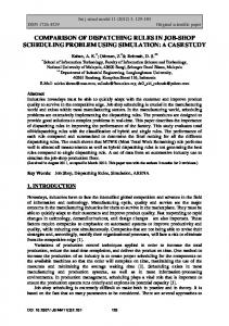
are randomly chosen points, and closer to each other than random points would be. In other words, the local optima are not randomly distributed, rather they tend to be clustered in a “central massif” (or “big valley” if we are minimising). This global structure has been observed in the abstract N K family of landscapes [14], and in many combinatorial optimisation problems, such as the traveling salesman problem [2], graph bipartitioning [15], and flowshop scheduling [17]. B. Hyper-heuristic Landscapes Our hyper-heuristic approach (described in section II), deals with two search spaces: (1) the search space of heuristics (HS), and (2) the search space of solutions to the problem at hand (P S). However, we have a single landscape, as the objective function value of a point in the heuristic search space, can only be known after calculating the objective value of the corresponding search point in the solution space. Figure 1 illustrates the two search spaces discussed and the two mappings involved, namely, g from a heuristic list to its corresponding problem solution, and f from the solution to the objective value. More formally, the objective function of a sequence of heuristics Aˆ in the heuristic space HS is given by the composition of g ˆ : HS → R. The hyper-heuristic and f , namely, f (g(A)) landscape is, therefore, defined as the triplet (HS, f (g), V ), where the first two components are defined as above, and V represents the neighbourhood produced by the minimal possible move operator on the heuristic search space (referred to as 1 − move). That is, the operator that substitutes one heuristic in the sequence by another (randomly selected) heuristic from the repository of low-level heuristics. IV. E XPERIMENTAL SETTINGS Two groups of experiments were conducted, the first group compares the performance attained by different problem representations (search spaces), defined by grouping decisions in different block sizes. A direct encoding of the problem based on permutations (i.e. a permutation search space), is a also explored. Four instances of the hybrid flowhsop problem were randomly generated with different numbers of jobs, n ∈ {50, 100}, and stages, m ∈ {5, 20}. The processing times were generated randomly using a discrete uniform distribution in the [10,100] interval. Note that the processing time of jobs in different stages may differ. The number of machines per stage were either 4 or 5, both with equal probability. For each problem instance, several ways of grouping decisions were studied. The representation that considers each decision individually, was always considered. In this representation there are n blocks of size 1 per stage; since there are m stages, there is a total of n × m decision blocks. Let us consider for example the case of 50 jobs, the distribution of decision blocks in stages is as follows: b , . . . , b , b , . . . , b , . . . , b50(m−1)+1 , . . . , b50m . 1  50 51  100    stage 1

stage 2

2009 IEEE Congress on Evolutionary Computation (CEC 2009)

Authorized licensed use limited to: UNIVERSITY OF NOTTINGHAM. Downloaded on September 14, 2009 at 10:37 from IEEE Xplore. Restrictions apply.

stage m

1875

g

f

Objective Function (makespan, completion times, max tardiness, etc)

h1 h2 h3 … hn

Heuristic space: sequence of dispatching rules

Problem space: flow shop schedules

Real numbers: objective function value of the schedule

Fig. 1. Hyper-heuristic mapping process from a sequence of heuristics to its fitness value. Two mappings are involved: g : HS → P S, and f : P S → R.

For n = 50, decisions were also grouped into 10 and 30 decision blocks per stage. When 10 blocks per stage are considered, each block contains 5 decisions, and when 30 blocks are considered, the first 20 blocks contain 2 decisions each whilst the last 10 one decision each. Similarly, for n = 100, blocks of size 25, 50, and 100 were used. A repository of 13 dispatching-rules were considered as low-level heuristics to be potentially assigned to each decision. These heuristics works as follows: whenever a machine is idle, select the job not yet scheduled and ready for processing (released from the previous stage) that best satisfies a certain criterion and assign it to the idle machine. The following rules were considered: minimum release time, shortest processing time, longest processing time, less work remaining, more work remaining, earliest due date, latest due date, weighed shortest processing time, weighted longest processing time, lowest weighted work remaining, highest weighted work remaining, lowest weighted due date and highest weighted due date. A standard GA with elitism was employed as the highlevel strategy searching on the different heuristic spaces, and the permutation space. The crossover operator implemented selects two chromosomes as parents, and sets any gene ci of the new chromosome with a probability α from the fittest parent and 1-α from the other. The mutation operator selects (n × m) × β random genes and substitutes them with a different randomly selected dispatching rule. Parameter β (0 < β < 1) controls the strength of mutation. The GA control parameters that produced the best results after an statistical tuning process [23] were used, namely: a population size of 100, and binary tournament selection with elitism. The algorithm selects the genetic operators independently to produce offspring; crossover with a probability of 0.9, and mutation with 0.1. The α and β parameters described above are set to 0.5 and 0.05, respectively. The stopping condition was set to 10 000 solution evaluations, and for each instance and representation 30 GA runs were conducted.

1876

V. R ESULTS Table I, summarises the average performance obtained after 30 GA runs for each representation and objective function on the four instances studied. The best obtained results for each instance and objective function are highlighted in bold font. Notice that the hyper-heuristic representation clearly outperformed the permutation representation in all cases, and the advantage of the heuristic representation is more noticeable for the sumW T objective function. Note also that grouping several decisions into blocks, that is, having shorter hyper-heuristic representations, seems to be favourable when considering a fixed computational effort. This was already observed in [23], where it was also found that considering too many or too few decision blocks per stage yielded comparably poor results. A large number of decision blocks per stage implies a larger search space, whereas very few decision blocks have very limited expression power, this may explain the observed behaviour. A. Landscape analysis It is clear from the results discussed above that the hyperheuristic search spaces offer an advantage when solving HFS problems. With the aim of gaining a better understanding of the structure of such search spaces, this section reports our statistical landscape analysis. 1) Heuristic space vs. permutation space: distribution of objective values: First, we compared the distribution of objective values, for both Cmax and sumW T , of a set of 10 000 randomly generated solutions on both the permutation and hyper-heuristic search spaces. The permutation space was sampled by generating random permutations which were decoded as schedules by assigning jobs in their order of appearance into the first machine to become available. The schedules were generated in such a way that there are no idle time windows on any machine that are large enough to process a job without delaying the completion time of any other job. Therefore, only active schedules were generated,

2009 IEEE Congress on Evolutionary Computation (CEC 2009)

Authorized licensed use limited to: UNIVERSITY OF NOTTINGHAM. Downloaded on September 14, 2009 at 10:37 from IEEE Xplore. Restrictions apply.

TABLE I

50 x 5

M EAN AND STANDARD DEVIATION OF 30 GA RUNS WITH BOTH OBJECTIVE FUNCTIONS (Cmax AND sumW T ), ON THE FOUR STUDIED INSTANCES . T HE DIFFERENT HEURISTIC REPRESENTATIONS ( NUMBER OF DECISION BLOCKS ), AND THE PERMUTATION REPRESENTATION , ARE REPORTED

120

.

100

80

60

60

40

40

20

20

m

representation

Cmax

stDev

sumWT

stDev

50

5

10 30 50 permutation

941.30 940.60 941.00 1042.90

3.74 3.10 3.86 11.60

41341.80 41391.20 41858.90 56107.20

562.78 745.09 392.51 2010.44

10 30 50 permutation

1755.30 1754.00 1756.50 2100.80

14.45 8.87 13.90 7.98

28481.20 28338.40 28565.50 65127.70

1272.17 728.53 1174.17 2305.55

25 50 100 permutation

1533.10 1523.80 1526.10 1610.20

3.03 2.86 4.33 7.05

250794.30 252856.80 256871.20 303553.80

3424.25 4217.34 4814.65 9260.10

80

25 50 100 permutation

2497.20 2504.70 2508.60 3072.20

6.84 11.43 11.70 20.98

195557.50 200104.20 208216.30 379926.20

4076.09 3686.10 6002.94 7898.86

40

100

5

20

0

0 5.72 7.53

50 x 5

50 x 20

140

140 hyperheuristic permutation

120

hyperheuristic permutation

120

100

100

80

80

60

60

40

40

20

20

0

0 9.98 10.7

12.8

14.4

18.7 19.5

100 x 5

22.5

24.9

100 x 20

160

200 hyperheuristic permutation

140

hyperheuristic permutation

180 160

120

140

100

120

80

100

60

80 60

40

40

20

20

0

0 16.2 16.8

18.9

21.3

26.8 28.1

32.6

36.9

Fig. 2. Distribution of Cmax values of random solutions of the hyperheuristic and permutation spaces

10.9

14.5

4.93 7.13

100 x 5

12.1

15.7

100 x 20

120

200 hyperheuristic permutation

100

hyperheuristic permutation

180 160 140 120

60

100 80 60 40

20

20 0

0 36.4 39.8

which are on average better than most random schedules [16]. The heuristic space was sampled by producing random sequences of dispatching rules, considering the maximum number of decision blocks (i.e. one heuristic per decision). Figures 2 and 3 show the empirical distributions obtained for the two objective functions (Cmax and sumW T ), respectively, on the four studied instances. Notice that for both objective functions the solutions represented as sequences of dispatching rules are significantly better than those represented as permutations. This is specially noticeable for the larger instances (i.e. with m = 20).

hyperheuristic permutation

100

80

n

20

50 x 20 120

hyperheuristic permutation

47.2

54.7

31.9 35.8

54.6

63.7

Fig. 3. Distribution of sumW T values of random solutions of the hyperheuristic and permutation spaces

2) Neighborhood of the best obtained heuristic sequences: In order to gain information about the ruggedness of the landscapes, Figures 4 and 5 illustrate the mean Cmax and sumW T values, respectively, (with 95% confidence interval) of all the 1-move neighbours of the best-known solution for each objective function. The horizontal axis denotes the position in the sequence, considering the elements from left to right, whilst the vertical axis the objective function value. A point in the plots with abscissa i represents the mean objective value of all the direct neighbours of the bestknown sequence, which differ from it in position i. Since there are 13 low-level heuristic in the heuristic space, each point in the plot represents, therefore, the average cost of 12 other sequences (each having a different heuristic in position i). These plots illustrate two interesting features of these heuristic landscapes. First, the landscapes are rugged, in that small differences in the heuristic list (1-moves) may produce a large difference in the solution objective value. Second, there is a strong positional bias in the heuristic search spaces, where changes on the list left-most positions have a much higher impact on the objective function as compared to the right-most positions. This relationship between the position in the list and the deterioration in cost is steady for the sumW T objective function (Figure 5), whereas for the Cmax function the relationship (Figure 4) is less structured but still has a decreasing trend. Another interesting observation is that some positions, especially with respect to the Cmax objective function (Figure 4), are neutral in that their modification do not produce changes in the cost value. These neutral positions tend to be located towards the right end of the sequences (Figure 5).

2009 IEEE Congress on Evolutionary Computation (CEC 2009)

Authorized licensed use limited to: UNIVERSITY OF NOTTINGHAM. Downloaded on September 14, 2009 at 10:37 from IEEE Xplore. Restrictions apply.

1877

50x5, rep. size 10

50x5, rep. size 30

50x5, rep. size 50

1060

980

960

1040

970

955

1020

950

960

1000

945

950

980

940

940

960 940

930

920

920 1

2

3

4

5

6

7

8

9 10

935 930 925 0

5

10

50x20, rep. size 10

15

20

25

30

1950 1900 1850 1800 1750 1700 2

3

4

5

6

7

8

9 10

1860 1840 1820 1800 1780 1760 1740 1720 0

5

10

100x5, rep. size 25

15

20

25

30

1580

1570

1570

1560

1560

1550

1550

1540

1540

1530

1530 1520

1510 10

15

20

25

1510 0

5 10 15 20 25 30 35 40 45 50

100x20, rep. size 25

100x20, rep. size 100

2620 2600 2580 2560 2540 2520 2500 2480 2460

2650 2600 2550 2500 2450 5

10

15

0 10 20 30 40 50 60 70 80 90 100

100x20, rep. size 50

2700

0

5 10 15 20 25 30 35 40 45 50 100x5, rep. size 100

1580

1520 5

0

100x5, rep. size 50

1610 1600 1590 1580 1570 1560 1550 1540 1530 1520 0

5 10 15 20 25 30 35 40 45 50 50x20, rep. size 50

1880 1860 1840 1820 1800 1780 1760 1740 1720 1

0

50x20, rep. size 30

20

25

2640 2620 2600 2580 2560 2540 2520 2500 2480 2460 0

5 10 15 20 25 30 35 40 45 50

0 10 20 30 40 50 60 70 80 90 100

Fig. 4. Mean and 95% confidence interval of the variation in the Cmax value of the all the 1-move neighbours of the best-known sequence. A point in the plots with abscissa i represents the mean cost of all the direct neighbours of the best-known sequence, which differ from it in position i. 50x5, rep. size 10

50x5, rep. size 30

65000

50x5, rep. size 50

48000 47000 46000 45000 44000 43000 42000 41000 40000

60000 55000 50000 45000 40000 1

2

3

4

5

6

7

8

9 10

48000 47000 46000 45000 44000 43000 42000 41000 40000 0

5

50x20, rep. size 10

10

15

20

25

30

45000 40000 35000 30000 25000 1

2

3

4

5

6

7

8

9 10

0

5

10

15

20

25

30

275000

275000

260000

255000

255000

250000 245000 20

25

250000 0 5 10 15 20 25 30 35 40 45 50

100x20, rep. size 25 240000 235000 230000 225000 220000 215000 210000 205000 200000 195000 190000

250000 240000 230000 220000 210000 200000 190000 0

5

10

15

20

0 10 20 30 40 50 60 70 80 90 100

100x20, rep. size 50

260000

25

100x20, rep. size 100 250000 245000 240000 235000 230000 225000 220000 215000 210000 205000 200000 195000

0 5 10 15 20 25 30 35 40 45 50

0 10 20 30 40 50 60 70 80 90 100

Fig. 5. Mean and 95% confidence interval of the variation in the sumW T value of the all the 1-move neighbours of the best-known sequence. A point in the plots with abscissa i represents the mean cost of all the direct neighbours of the best-known sequence, which differ from it in position i.

B. Fitness-distance correlation analysis The fitness-distance analysis requires knowledge of the optimal solution. However, given that the optimal solution is not generally known, many studies in the literature use the best-known solution instead. For the analysis, we considered

1878

5

10 30 50 permutation

0.580 0.691 0.760 0.483

0.637 0.585 0.615 0.133

0.618 0.650 0.669 0.863

0.741 0.841 0.841 0.775

20

10 30 50 permutation

0.634 0.672 0.680 0.180

0.774 0.699 0.758 0.047

0.802 0.595 0.704 0.745

0.894 0.793 0.862 0.674

5

25 50 100 permutation

0.744 0.750 0.909 0.195

0.580 0.577 0.685 0.085

0.533 0.545 0.605 0.898

0.877 0.927 0.922 0.788

20

25 50 100 permutation

0.670 0.780 0.787 0.483

0.647 0.811 0.834 0.291

0.648 0.790 0.900 0.823

0.870 0.878 0.939 0.664

100

fdc

265000

260000

15

50

270000

265000

10

100x5, rep. size 100 280000

270000

5

representation

0 5 10 15 20 25 30 35 40 45 50

100x5, rep. size 50 280000

sumWT fdc fdcls

m

44000 42000 40000 38000 36000 34000 32000 30000 28000 26000

100x5, rep. size 25 295000 290000 285000 280000 275000 270000 265000 260000 255000 250000 0

0 5 10 15 20 25 30 35 40 45 50

Cmax fdcls

n

50x20, rep. size 50

44000 42000 40000 38000 36000 34000 32000 30000 28000 26000

50000

TABLE II F ITNESS DISTANCE CORRELATION COEFFICIENT WITH RANDOM SAMPLING (f dc) AND LOCAL SEARCH SAMPLING (f dcls). REPRESENTATION ARE SHOWN .

50x20, rep. size 30

55000

both a set of random sequences and a set of empirically generated local optima. The set of random sequences where generated as follows. For a given instance, let x∗ be the bestknown solution in the heuristic search space, referred to as the optimum and obtained after the experiments reported in Table I. In order to have a wide distribution of distances to the optimum, a fixed number of solutions (10 in our experiments) were randomly generated at each distance i, for i = 1, . . . , n×m, away from x∗ . Thus, 10×(n×m) random sequences were produced for each instance, representation and objective function. The local optima were produced using a next-improvement local-search algorithm, based on the 1move neighbourhood, and starting from the set of random solutions described above. As the distance metric between the heuristic sequences, we used the Hamming distance, that is, the number of positions in which two sequences differ. Notice that our low-level heuristics set contains 13 elements {h1 , h2 , h3 , . . . , h13 }, but there is no order relationship between them. That is, h1 is not farther away from h13 than it is from h2 ; the indexing convention for heuristics is arbitrary. Therefore, Hamming distance is a good metric for gauging the distance between two sequences of heuristics.

Table II, illustrates the fitness distance correlation coefficients for both the random sample (f dc) and the local optima (f dcls) sample of solutions, with respect to the two objective functions. We may observe that all the hyper-heuristic representations show a high positive correlation between the cost and distance to the optimum for both random sequences and local optima (in the range of 0.580 to 0.927), which predicts an easy search. The correlation coefficients of the permutation representation are, on the other hand, much lower, when considering the Cmax objective function, as compared to the sumW T function. With respect to the the hyper-heuristic spaces high f dcls values implies that the lower the cost the closer the local optima are to the global optimum (or best-known solution). It also suggests a big valley structure of the underlying

2009 IEEE Congress on Evolutionary Computation (CEC 2009)

Authorized licensed use limited to: UNIVERSITY OF NOTTINGHAM. Downloaded on September 14, 2009 at 10:37 from IEEE Xplore. Restrictions apply.

50x5, perm. rep.

Cmax

50x5, rep. size 50

Cmax

Cmax

50x5, rep. size 30

Cmax

50x5, rep. size 10

50x20, perm. rep.

Cmax

distance to optimum

50x20, rep. size 50

Cmax

distance to optimum

50x20, rep. size 30

Cmax

distance to optimum

50x20, rep. size 10

Cmax

distance to optimum

100x5, rep. size 25

100x5, rep. size 50

100x5, rep. size 100

100x5, perm. rep.

Cmax

distance to optimum

Cmax

distance to optimum

Cmax

distance to optimum

Cmax

distance to optimum

100x20, rep. size 25

100x20, rep. size 50

100x20, rep. size 100

100x20, perm. rep.

distance to optimum

distance to optimum

Cmax

distance to optimum

Cmax

distance to optimum

Cmax

distance to optimum

Cmax

distance to optimum

distance to optimum

distance to optimum

Fig. 6. Fitness-distance correlation scatter-plots of local optima (Cmax objective function) of the landscapes studied.

VI. S UMMARY AND C ONCLUSIONS Hyper-heuristics approaches differ from other heuristic search techniques in that they operate on a search space of heuristics, rather than directly on a search space of solutions to the underlying problem. Our motivation was, therefore, to study the structure of an example of such

50x5, perm. rep.

sumWT

50x5, rep. size 50

sumWT

50x5, rep. size 30

sumWT

sumWT

50x5, rep. size 10

50x20, perm. rep.

sumWT

distance to optimum

50x20, rep. size 50

sumWT

distance to optimum

50x20, rep. size 30

sumWT

distance to optimum

50x20, rep. size 10

sumWT

distance to optimum

100x5, rep. size 25

100x5, rep. size 50

100x5, rep. size 100

100x5, perm. rep.

sumWT

distance to optimum

sumWT

distance to optimum

sumWT

distance to optimum

sumWT

distance to optimum

distance to optimum

100x20, rep. size 25

100x20, rep. size 50

100x20, rep. size 100

100x20, perm. rep.

distance to optimum

distance to optimum

sumWT

distance to optimum

sumWT

distance to optimum

sumWT

distance to optimum

sumWT

landscape (as discussed in Section III-A). In addition to the f dcls coefficients, fitness-distance scatter plots (shown in Figures 6, and 7) provide useful information about the landscapes for both the Cmax , and sumW T cost functions, respectively. Notice that for the hyper-heuristic representation, the plots for all instances and representation lengths have a similar general outlook: the costs of local optima and distances to the optimum show a clear positive correlation. The scatter plots for the permutation presentation (rightmost column of Figures 6, and 7) show a different overall picture. For the Cmax objective function (Figure 6) there is no observable correlation between the cost of local optima and their distances to the optimum, while for the sumW T function (Figure 7), a positive correlation seems to hold, but only for the best local optima; that is, those with a lower objective function values. There are, in this case, a large number of low-quality local optima that show no clear fitness-distance correlation and are, therefore, randomly located in the search space. Finally, notice that for some instances (i.e. that with n = 100, m = 5) , the scatter plots suggest that there are several (different) local optima having the same or very similar fitness as the best-known solution, so there seems to be a set of optimal solutions (instead of a single optimum) located in a plateau, which suggest the presence of neutrality in these landscapes.

distance to optimum

distance to optimum

Fig. 7. Fitness-distance correlation scatter-plots of local optima (sumW T objective function) of the landscapes studied.

heuristic search spaces. We formalised the notion of hyperheuristic landscapes and performed a landscape analysis of the heuristic search space induced by a dispatching-rulebased hyper-heuristic for the hybrid flowshop scheduling problem. This hyper-heuristic operates upon a set of dispatching rules widely used in production scheduling. Specifically, we conducted a fitness-distance correlation analysis of the landscapes of four instances of the hybrid flowshop problem, and employed additional visualisation techniques. We considered two different objective functions, and several hyper-heuristic representation sizes. A permutation based direct representation was also studied for the sake of comparisons. Our study confirmed the suitability of heuristic search spaces, and therefore the relevance of hyper-heuristic approaches. The prominent features of the studied landscapes can be summarised as follows: • Big valley structure: the cost of local optima and their distances to the global optimum (best-known solution) are correlated, which suggests that these landscapes has a globally convex or big valley global structure. • Large number of local optima: the landscapes contain large number of distinct local optima, many of them of low quality. • Existence of plateaus (neutrality): many local optima are located at the same level (height) in the search space, that is, they have the same cost value. • Positional bias: left-most positions in the heuristic list have a much greater impact on the produced solution cost. This implies that the decisions at the early stages of the scheduling process are more important. We suggest that search algorithms that explicitly exploit the features described above, will enhance the search on this

2009 IEEE Congress on Evolutionary Computation (CEC 2009)

Authorized licensed use limited to: UNIVERSITY OF NOTTINGHAM. Downloaded on September 14, 2009 at 10:37 from IEEE Xplore. Restrictions apply.

1879

type of heuristic search space. These performance predictions should be tested in future work. Moreover, similar and more advanced landscape analysis techniques should be conducted on both larger set of instances and types of production scheduling problems. R EFERENCES [1] A. Allahverdi and F. S. Al-Anzi. Scheduling multi-stage parallelprocessor services to minimize average response time. Journal of the Operational Research Society, 57:101–110, 2006. [2] K. D. Boese, A. B. Kahng, and S. Muddu. A new adaptive multi-start technique for combinatorial global optimizations. Operations Research Letters, 16:101–113, 1994. [3] E. K. Burke, E. Hart, G. Kendall, J. Newall, P. Ross, and S. Schulenburg. Hyper-heuristics: An emerging direction in modern search technology. In F. Glover and G. Kochenberger, editors, Handbook of Metaheuristics, pages 457–474. Kluwer, 2003. [4] E. K. Burke, B. McCollum, A. Meisels, S. Petrovic, and R. Qu. A graph-based hyper-heuristic for educational timetabling problems. European Journal of Operational Research, 176:177–192, 2007. [5] J. Carlier and E. Neron. An exact method for solving the multiprocessor flow-shop. RAIRO Research Op´erationale, 34:1–25, 2000. [6] J. Cheng, Y.i Karuno, and H. Kise. A shifting bottleneck approach for a parallel-machine flow shop scheduling problem. Journal of the Operations Research Society of Japan, 44:140–156, 2001. [7] U. Dorndorf and E. Pesch. Evolution based learning in a job shop scheduling environment. Computers and Operations Research, 22(1):25–40, 1995. [8] H.L Fang, P. Ross, and D. Corne. A promising genetic algorithm approach to job shop scheduling, rescheduling, and open-shop scheduling problems. In S. Forrest, editor, Fifth International Conference on Genetic Algorithms, pages 375–382, San Mateo, 1993. Morgan Kaufmann. [9] H. Fisher and G. L. Thompson. Probabilistic learning combinations of local job-shop scheduling rules. In Factory Scheduling Conference, Carnegie Institue of Technology, May 10-12 1961. [10] H. Fisher and G. L. Thompson. Probabilistic learning combinations of local job-shop scheduling rules. In J. F. Muth and G. L. Thompson, editors, Industrial Scheduling, pages 225–251, New Jersey, 1963. Prentice-Hall, Inc. [11] R. R. Garc´ıa and C. Maroto. A genetic algorithm for hybrid flow shops with sequence dependent setup times and machine elegibility. European Journal of Operational Research, 169:781–800, 2006. [12] J. N. D. Gupta. Two-stage hybrid flow shop scheduling problem. Operational Research Society, 39:359–364, 1988. [13] T. Jones. Crossover, macromutation, and population-based search. In L. J. Eshelman, editor, Proceedings of the Sixth International Conference on Genetic Algorithms, pages 73–80, San Francisco, CA, 1995. Morgan Kaufmann. [14] S. A. Kauffman. The Origins of Order: Self-Organization and Selection in Evolution. Oxford University Press, 1993. [15] P. Merz and B.Freisleben. Fitness landscapes, memetic algorithms, and greedy operators for graph bipartitiioning. Evolutionary Computation, 8(1):61–91, 2000. [16] M. Pinedo. Scheduling Theory, Algorithms and Systems. Prentice Hall, 2002. [17] C. R. Reeves. Landscapes, operators and heuristic search. Annals of Operations Research, 86:473–490, 1999. [18] C. R. Reeves. Fitness landscapes, chapter 19. In E. K. Burke and G. Kendall, editors, Search Methodologies: Introductory Tutorials in Optimization and Decision Support Techniques, pages 587–610. Springer, 2005. [19] D. L. Santos, J. L. Hunssucker, and D. E. Deal. FLOWMULT: Permutation sequences for flow shops with multiple processors. Journal of Information and Optimization Sciences, 16:351–366, 1995. [20] R. H. Storer, S. D. Wu, and R. Vaccari. New search spaces for sequencing problems with application to job shop scheduling. Management Science, 38(10):1495–1509, 1992. [21] R. H. Storer, S. D. Wu, and R. Vaccari. Problem and heuristic space search strategies for job shop scheduling. ORSA Journal of Computing, 7(4):453–467, 1995.

1880

[22] J. A. Vazquez-Rodriguez, S. Petrovic, and A. Salhi. A combined metaheuristic with hyper-heuristic approach to the scheduling of the hybrid flow shop with sequence dependent setup times and uniform machines. In Proceedings of the 3rd Multidisciplinary International Scheduling Conference: Theory and Applications (MISTA 2007), 2007. [23] J. A. V´azquez-Rodr´iguez, S. Petrovic, and A. Salhi. An investigation of hyper-heuristic search spaces. In Dipti Srinivasan and Lipo Wang, editors, 2007 IEEE Congress on Evolutionary Computation, pages 3776–3783, Singapore, 25-28 September 2007. IEEE Computational Intelligence Society, IEEE Press. [24] J. A. V. Rodr´iguez. Meta-hyper-heuristics for hybrid flow shops. Ph.D. thesis, University of Essex, 2007. [25] A. Vignier, D. Dardilhac, D. Dezalay, and S. Proust. A branch and bound approach to minimize the total completion time in a k-stage hybrid flowshop. In Proceedings of the 1996 Conference on Emerging Technologies and Factory Automation, pages 215–220. IEEE press, 1996. [26] S. Wright. The roles of mutation, inbreeding, crossbreeding and selection in evolution. In D. F. Jones, editor, Proceedings of the Sixth International Congress on Genetics, volume 1, pages 356–366, 1932.

2009 IEEE Congress on Evolutionary Computation (CEC 2009)

Authorized licensed use limited to: UNIVERSITY OF NOTTINGHAM. Downloaded on September 14, 2009 at 10:37 from IEEE Xplore. Restrictions apply.