Displacement and Squeeze Operators of a Three-Dimensional Harmonic Oscillator and Their Associated Quantum States
Mehdi Miri, Sina Khorasani School of Electrical Engineering Sharif University of Technology P. O. Box 11365-9363 Tehran, Iran Fax: +9821-6602-3261 Email:
[email protected]
Abstract We generalized the squeeze and displacement operators of the one-dimensional harmonic oscillator to the three-dimensional case and based on these operators we construct the corresponding coherent and squeezed states. We have also calculated the Wigner function for the three-dimensional harmonic oscillator and from the analysis of time evolution of this function, the quantum Liouville equation is also presented. Further properties of the quantum states including Mandel’s parameters are discussed as well.
Keywords: coherent states, phase space, squeezed states, operator algebra
1
and quadrature squeezing
1. Introduction The operator theory of harmonic oscillators [1] constitutes the groundwork of the elaborate quantum optical theory of photons. The quantization of electromagnetic radiation can be explained elegantly in terms of creator and annihilator operators, which operate on the corresponding energy levels [2-4]. Due to the second-order potential of harmonic oscillators, they can easily provide a direct bridge between classical optics and quantum optics through the phase-space Wigner functions [5], which are of extreme importance in the tomography of classical and non-classical lights [6-8]. Following the definition of coherent states put forward by Glauber [2-4], as the eigenstates of the annihilator operator, many studies have been done in order to generalize the concept of coherent states and the so-called squeezed states [5, 9]. Among these include an alternative definition of the generalized photon coherent states [10], which introduce a modification of the squeezing operator to describe higherorder interactions. In another report [11] the authors consider the generalization of coherent states and their superpositions connected through unitary transformations, where the transformation maps the ground state of the harmonic oscillator (vacuum state) onto an arbitrary superposition of
2 coherent states.
Since the successful demonstration of squeezed states of light in 1985 by Bell Laboratories [12], squeezed states have attracted much interest because of their possibility to significantly suppress the quantum noise, which is generally believed to be originated by the zero-point fluctuations of the vacuum [5]. Currently, squeezed states are routinely produced at laboratories using both solid-state and semiconductor lasers [13] and in high- cavities [14]. Similarly, generalizations or extensions to the concept of squeezed states have been considered in numerous researches. Nieto [15] was the first to discuss the explicit functional forms for the squeeze and time-displacement operators and their applications, as successive multiplications of exponentials of simple operators. Bialynicki-Birula [16,17] presented a discussion of squeezed states of a generalized infinitedimensional harmonic oscillator, when the ground state wave function takes on a Gaussian form. He furthermore presented the corresponding Wigner function and discussed its relativistic properties. As another generalization of the simple one-dimensional harmonic oscillator, the problem of damped harmonic oscillator because of its time-dependent Hamiltonian was proposed and considered by Um et. al. [18], and they presented closed form expressions for squeeze and displacement operators. Also, Sohn and Swanson [19] have recently obtained exact transition elements of the squeezed harmonic oscillator when
2
the generalized Hamiltonian describes two-photon processes, using Bogoliubov transformations. Fakhri [20] considered the three-dimensional (3D) harmonic oscillator and Morse potentials, and showed that the constructed Heisenberg Lie superalgebras would lead to multiple supercharges. In his analysis, he analyzed the 3D harmonic oscillator in the spherical system of coordinates. Finally, Fan and Jiang [21] have constructed three mutually commuting squeeze operators, which are applicable to three-mode states. In this paper, we revisit the 3D harmonic oscillator and obtain generalized expressions for the corresponding coherent and squeezed states, starting from the Cartesian coordinates in which the harmonic oscillator can be easily factorized. We also present closed-form simple expressions which explicitly represent the corresponding displacement and squeeze operators, and the corresponding generalized Mandel’s
parameter is obtained for the generalized squeezed state in the form of a vector.
We show that how proper definition of vector operators and variable could greatly simplify the notations of operators and eigenstates.
2. Coherent states and the displacement operator 2.1. Wigner function for 3D harmonic oscillator We can calculate wave function of three-dimensional (3D) harmonic oscillator directly from the Schrödinger equation, with the diagonalized potential given by
2.1
2
. Now let | , ,
Here, without loss of generality one may assume that
denote the
energy eigenstates of 3D harmonic oscillator, hence for the corresponding annihilation and creation operators we have | , ,
√ |
| , , | , ,
1, ,
2.2
a
√ | ,
1,
2.2
b
√| , ,
1
2.2
c
| , ,
√
1|
1, ,
2.2
d
| , ,
√
1| ,
1,
2.2
e
| , ,
√
1| , ,
2.2
f
3
1
Hence, the eigenfunctions will be
1
| , ,
Ψ
√2
!
1 2
exp
! !
H
H
H
2.3
⁄ . We can find the corresponding Wigner function for this system from the definition of
where
the Wigner function as
W|
Here,
1
,
, ,
exp
2
·
k represents the dummy integration variable. In the
is the density operator and | , ,
case of pure state with
W|
, ,
1
,
, , | gives
exp
2
2.4
·
Ψ
Ψ
2.5
The Wigner function of 3D harmonic oscillator will take the form
W|
, ,
1
, L
in which L
exp
2
L
2
L 2
2.6
is the Laguerre function of order ; see appendix A for the detailed derivation of (2.6). For
the generation of coherent states, we must apply a suitable displacement operator to the ground state of 3D harmonic oscillator. In doing so, we need to generalize the method of [15] in construction of 3D displacement operator. 2.2. Construction of coherent state The ground state of a 3D harmonic oscillator is given by
4
|
Ψ
in which the ground state |
1 2
exp
2.7
0,0,0 . Now we define the
is defined using the null integer triplet
displacement operator as exp
exp
exp , with
Here, the displacement vector
will be shown, the order of displacements along , , and
,
2.8 , and
being complex constants. As
is irrelevant. This is because of the obvious
relations ,
,
,
0, ,
,
, ,
2.9
0,
2.9
In trying to find a compact form for this operator we start from the Baker-Campbell-Hausdorff relation [5], which reads
exp
exp
exp
exp
1 2
,
2.10
given that
,
,
,
,
0
2.11
Hence the displacement operator is simplified into the compact form exp
·
·
2.12
where the vector creation and annihilation operators are defined by
5
2.13
a
2.13
b
to the ground state |
The application of the displacement operator | where |
|
results in
2.14
is defined as the generalized coherent state in 3D. Also, from the properties of
and
one can
further observe that 1 2
exp
The position representation of |
|
·
exp
exp
·
·
2.15
will be
1 2
exp
√2
√2 1 2
exp
√2
2.16
√2
The direct application of the displacement operator also can be simply shown to equally result in the triple infinite series of the generalized coherent state as
|
|
exp
exp
1 2
·
1 2
·
1 ! ! !
, ,
·
! ! !
, ,
·
| , ,
·
|
2.17
2.3. Over-completeness of coherent states As one of the important properties of coherent sates we can examine the over-completeness of the proposed coherent sates. A set of states are called over-complete if they form a complete set and are not orthogonal. We first consider the completeness of coherent states: ∞
∞
| ∞
∞
|
| ∞
|
exp ∞
6
1 2
·
exp
1 2
·
∞
, ,
| , !
, ,
Re
where
∞
Im
;
,
, , |
2.18
! ! ! ! !
, , . Using the change of variables:
exp
;
, ,
2.19
results in: ∞
, ,
∞
| , !
, ,
, , |
,
! ! ! ! !
∞
exp ∞
;
exp
It is known that
2
exp
2.20
2
, so using
;
, , , we get:
∞
|
|
∞ ∞
, ,
| ,
, !
,
, |
! !
∞
∞
exp
exp
∞
which can be easily simplified by using the identity ∞
exp
∞
∞
∞ exp ∞
! into the expression:
2.21
∞
| ∞
∞
|
| ,
,
,
, |
2.22
, ,
Therefore the proposed coherent sates constitute a complete set. Now we examine their non-orthogonality by considering the inner product of two different coherent states |
7
and |
:
|
exp
1 2
·
exp
exp exp exp
∞
,
· , ,
!
, ,
, | , ,
! ! ! ! !
∞
1 2
·
1 2
·
1 2
∞
1 2
·
!
, ,
·
·
·
! !
· 1 2
exp
·
2.23
Hence, we obtain the squared magnitude of the inner product as: | |
|
exp
·
0
2.24
which declares that 3D coherent states are not orthogonal, but their inner product tends to vanish, when |
| is sufficiently large. Equations (2.22) and (2.24), establish, therefore, that the proposed coherent
sates are over-complete.
2.4. Quantum Liouville equation in 3D Now we attempt to find the quantum Liouville equation for the generalized 3D harmonic oscillator system of interest. So we start from time evolution of our six-dimensional (6D) Wigner function. We have the Von Neumann equation for the time evolution of density operator as [1,5]
,
with
2.25
representing the Hamiltonian of the 3D harmonic oscillator. Starting from this equation we can
show that 1 2
1 2
1 2
,
1 2
With substitution of (2.19) in the definition of Wigner function we get
8
2.26
W , ,
Here,
and
2.27
respectively correspond to kinetic and potential energies in terms of Moyal functions and
introduce a Fourier transform as in [5]. The derivation closely follows the approach in [5], however, we employ the generalized 3D expressions for functions and operators. Hence,
and
will be given by the
expressions
1
1 2
exp
2 1 2
, ,
· 1 2
,
, , 2.28
a
and 1
exp
2 1 2
, ,
The potential energy operator
· 1 2
,
, , 2.28
b
is similarly defined as in [5]. Now we need to calculate
and
in terms
of the Wigner function and its higher-order derivatives. First we consider the kinetic energy term, which gives rise after some mathematical manipulations to the following equation for the kinetic energy term 1
·
W , ,
2.29
Now consider potential energy term. From the 3D Taylor expansion near , we have:
1 2
1 !
1 · 2
Therefore we obtain
9
2.30
1 2
1 2
2
2
·
!
2.31
and
1 2
1 2
2
2
·
1 !
2.32
We finally have the closed-form expression
2
1 2
·
1 !
W , ,
2.33
With substitution of (2.29) and (2.33) in (2.27) we get the Liouville's equation for the time-evolution of the Wigner function in 3D in the compact form
1
·
W , ,
2
1 2
1 !
·
W , ,
For the 3D harmonic oscillator in general case, the potential
2.34
is second-order in . So for the
harmonic oscillator, the right-hand-side of the Liouville's equation is equal to zero. Hence, the quantum Liouville's equation for 3D harmonic oscillator will be simply 1
·
·
W , ,
0
2.35
2.5. Time Evolution of Coherent State The Hamiltonian of 3D harmonic oscillator is time independent, so for the temporal evolution of the coherent state we can write down
|Ψ
| , ,
exp , ,
10
, , |Ψ
0
2.36
Defining the expansion coefficients as Ω
, , |Ψ
, ,
0
2.37
we get after some algebra
Ω
, ,
exp
1 2
·
2.38
√ ! ! !
On the other hand 3 | , , 2
| , ,
2.39
After simplifying we have
|Ψ
exp
3 2
√ ! ! !
, ,
exp
1 2
3 2
Ψ
| , ,
·
2.40
from which we obtain
|Ψ
exp
2.41
From this relation we see that the time evolution of coherent state is also a coherent state, and also after one period
of oscillation, the state vector phase change is
3 .
2.6. Position representation of coherent state In the below we try to find a compact form for position representation of coherent state of 3D harmonic oscillator. This results in
11
|Ψ exp
1 3 2
1 2
exp
·
·
exp √2
·
2.42
Using the definitions √2
Re Im
√2 3 2
Φ
· 2
1
·
2
1 2
·
2.43
a
2.43
b
2.43
c
Re
·
2.43
d
Finally, the complete form of position space representation of coherent state is Ψ
,
|Ψ exp
2
·
exp
for real
Here, as for the case in 1D problem
·
exp
Φ
2.44
will take on real values, otherwise it will be complex.
3. Squeezed states and the squeeze operator Now we try to find functional form of squeeze operator and squeezed state of 3D harmonic oscillator and position representation of this squeezed state. For 1D case, the squeeze operator is defined as
exp
1 2
1 2
where in general is a complex number
12
3.1
| |
3.2
Expanded form of 1D squeezing operator is therefore
exp
1 2
tanh| |
sech| | !
sech | |
1
1 2
exp
tanh| |
3.3
If we use notation of [15] as 1 √2 ̂
1 √2
3.4
a
3.4
b
the new form of squeezing operator will take the form
exp
1 2
3.5
2
In the expanded form we have
exp
sinh| | 2| |
exp
ln
exp
sinh| |
3.6
2| |
where
cosh| |
s sinh| | | |
| |
cos
2
| |
sin
2
3.7
In generalization of this concept to 3D case we consider 3D squeezing as independently squeezing of wave function of harmonic oscillator in the three
,
, and
dimensions. So for the 3D harmonic
oscillator this method can be applied directly resulting as 3.8
13
,
Here,
operate only on , , and
, and
dimensions, respectively, and hence the
order of their appearance is irrelevant as will be shown shortly. We have 1 2 1 exp 2 1 exp 2
1 2 1 2 1 2
1 2
1 2
exp
3.9
a
3.9
b
3.9
c
Therefore
exp
1 2
1 2
exp
1 2
1 2
exp
3.10
Now let the following definitions hold
̂
1 √2 ̂
1 √2
3.11
a
3.11
b
, , . We furthermore we can show that
in which
,
,
,
,
0
3.12
where ,
, ,
,
,
With subsequent use of (3.12) we can show that
,
,
14
0
3.13
a
,
,
,
, ,
,
,
,
0
,
,
0
,
,
,
0
3.13
b
3.13
c
3.13
d
, ,
From equation (3.13) and after using (3.12), and the Baker-Campbell-Hausdorff relation one can easily show that the squeeze operator in 3D takes the more compact form
exp
1 2
3.14
With the help of the definitions of vectors 3.15
a
3.15
b
3.15
c
we can find a rather compact form for squeezing operator as
exp
1 2
3.16
The following commutation relations clearly hold
,̂ ̂
̂, ̂
,
̂ , ̂
, ,
, ,
from which the alternate form of the squeeze operator is obtained
15
̂ , ̂
0
3.17
exp
1 2
·
·
3.18
In the last equation we have used the short-hand notations Re
3.19
a
Im
3.19
b
̂ ̂
3.19
c
3.19
d
3.19
e
4. Construction of squeezed states For the generation of squeezed state we must apply the squeeze operator and then coherent operator on the ground state of harmonic oscillator. Here in this process, we use the notation of [15] employed in (3.6). This results in |
| , |
Notice that
3.20
represents the squeezed vacuum. Following the previous definitions and after some
algebra we reach at the position representation of the squeezed state as Ψ
| , 1
exp
2
exp
·
1
exp
1
exp
Here,
·
2 1
exp
2 ,
2
, and
1
2
, where
3.22
16
a
3.21
sinh 2 exp
3.22
b
, ,
and
are elements of the vectors
and
⁄√2, and
defined in (3.19),
3.23 cosh
sinh
exp
cos
2
tan
a sin
exp 3.23
2
3.23
b
c
, , For the detailed derivation of the (3.21), please refer to the Appendix B. 4.1. Further properties of squeezed states In this section we will consider two important properties of squeezed states; quadrature squeezing parameter and Mandel’s
parameter. For 1D squeezed states these two are defined as scalars, while for
the proposed 3D states we define the generalized quadrature squeezing and Mandel’s vector form. In the following we start with Mandel’s Mandel’s
parameters in the
parameter.
“as a measure of departure of the variance of the photon number n from the variance of a
Poisson process” was first proposed and calculated by Mandel [22, 23]. Δ
For an arbitrary state,
;
Δ
3.24
can be negative, zero, or positive, which respectively infers a super-Poissonian,
Poissonian or sub-Poissonian statistics [24]. It should be added here that Mandel has shown that, one should expect the squeezed states to show sub-Poissonian photon statistics through normal detection schemes [23].
17
For our 3D squeezed states, we define a vectorial Mandel’s Mandel’s
,
parameter,
,
where
is the
parameter related to squeezing in the direction. Note that the proposed squeezed state here
can also be represented as the multiplication of three squeezed sates: Ψ
1
Ψ
, ,
Ψ
exp
Ψ
3.25
1
exp
exp
2
y Ψ
Ψ
;
2
, ,
3.26
Now by using the results of [24] for 1D squeezed state, we can show that: | |
cos | |
and
sin sinh
2 sinh
cosh
1;
, ,
3.27
are defined in (3.23) and | |
1 2
3.28
tan
3.28 3.28
2 , , In this case, Mandel’s
parameter for squeezing in each direction (
;
, , ) can be negative, zero
or positive which means the statistics of squeezed states in that particular direction is super-Poissonian, Poissonian or sub-Poissonian respectively. Surface plots of the Mandel’s Figure 1, as a function of dependence on the angle cosh
sinh
and , while retaining when
parameter are illustrated in
as a constant. As it can be seen, there is no
0. For this special case, one can easily check from (3.27) that
.
Similarly, we can also define vectorial quadrature operator: 1 2
18
3.29
a
1 2 where
and
3.29
b
are defined in (2.13). In 1D squeezed state variances of quadrature operators are measures 1/2
of squeezing. In fact for a 1D squeezed state with quadrature
and
1/2
operators squeezing exists if [25]: 1 4
Δ
1 4
Δ
3.30
Again for our 3D squeezed state, we can calculate variances of elements of vectorial quadrature operators from the results of [24] for 1D squeezed state:
Δ
Δ
, Δ
, Δ
3.31
Δ
Δ
, Δ
, Δ
3.31
Δ Δ
1 4 1 4
cos sin
sin
2
cos
2
3.31
2
3.31
2
, , , , , , squeezing exists if:
Thus for 3D squeezed state, in direction
Δ
1 4
Δ
1 4
;
Plots of squeeze parameters (3.31c) and (3.31d) versus
, ,
and
3.32
are shown in Figs. 2 and 3, respectively as
surface and contour diagrams. As it can be seen, squeezed states happen over the domains in which (3.32) 1 4
holds, and any of the squeeze parameters fall under . Evidently, the transformation subplots for Δ
and Δ
switches the
, due to the algebraic forms of the expressions (3.31c) and (3.31d).
19
Furthermore, Figure 4 shows the domain of squeezed Δ
versus de-squeezed Δ
,
states,
,
respectively, filled in with color contours, and left blank. The borders could be explicitly found by solving (3.31c) and (3.31d) for Δ
. This gives after simplifications to the fairly compact expression
,
tan
;
2
, ,
3.32
which defines the borders separating the squeezed and de-squeezed states.
5. Conclusions In this paper, we presented new closed-form expressions for coherent states and squeeze operators of a generalized harmonic oscillator potential in three spatial dimensions. We defined proper creation and annihilation operators and succeeded in presenting simple expressions for the corresponding displacement and squeeze operators.
Appendix A: Derivation of Wigner function of 3D harmonic oscillator The position representation of | , ,
| , ,
Ψ
state 3D harmonic oscillator reads:
1 √2
!
1 2
exp
! !
H
H
H
A. 1
Placing the above in the definition of Wigner function in (2.5) gives:
W|
, ,
1
,
2 ·
1
H
exp
! !
1 2
exp 1 2
!
2
1 2
exp 1 2 1
1 2
H ·
·
20
1 2
H H .2
1 2
H H
1 2
1 2
exp
! 1 2
1 2
exp 1 2
H
1
1 2
exp 1 2
H
exp √ 2
exp
1 2
1 2
H
1 2
exp
1 2
1 2
H
1 2
1 2
exp
1 2
1 2
H
.5
we have:
1 4
exp
!
1 2
. By changing
Consider for example the first integral
1 2
.4
exp
!
1 2 .3
exp
!
2
1 2
H
1 2
exp
1 2
1 2
.6
and now by using the algebraic manipulation: 1 4
1 2
2
and change of variables
2
.7
2 :
exp
1 2
!
√ exp
H
.8
H
from symmetry of Hermite polynomials we know that H
21
1 H
. So
exp
1
1 2
!
√ H
exp
H
.9
Also it is known that:
1 2
1 !√
exp
H
H
L
2
. 10
where L is the Laguerre polynomial of order n. Therefore
1 exp
L
2
. 11
Repeating the same procedure for Iy and Iz results in:
W|
, ,
1
, L
exp
2
L
2
L 2
. 12
Appendix B: Derivation of Position representation of 3D squeezed state From (2.8) and by using the notation of [15] we can write the 3D displacement operator in this new form:
exp
2
exp
̂ exp
22
;
, ,
.1
where ̂ and
are defined in (3.11) and
and
are define above the (3.23). Furthermore as it is shown
in (3.10) 3D squeeze operator can also be shown to be:
exp
1 2 ̂
̂
;
, ,
.2
Our proposed squeezed state is constructed from ground state of a 3D harmonic oscillator (vacuum state) as in (3.20). So its position representation can be calculated from: |
| ,
Ψ 1
exp
1 2
.3
From the previously used commutation relation it is obvious that:
Ψ
1
exp
1 2
1 2
exp
exp
1 2
B. 4
Using [15] gives: 1 2
1
exp
2
1
exp
exp
2
.5
, , which directly results in the position representation of the squeezed state as:
Ψ
1
exp
2 exp
·
exp
1
exp
·
2
1
exp
2
23
1 2
B. 6
References [1]
Levi, A. Applied Quantum Mechanics; Cambridge University Press: New York, 2003.
[2]
Glauber, R. J. Photon Correlations. Phys. Rev. Lett. 1963, 10, 84-86.
[3]
Glauber, R. J. The Quantum Theory of Optical Coherence. Phys. Rev. 1963, 130, 2529-2539.
[4]
Glauber, R. J. Coherent and Incoherent States of the Radiation Field. Phys. Rev. 1963, 131, 27662788.
[5]
Schleich, W. P. Quantum Optics in Phase Space; Berlin: Wiley-VCH Verlag, 2001.
[6]
Meng, X.-G.; Wang, J.-S.; Fan, H.-Y. Wigner function and tomogram of the excited squeezed vacuum state. Phys. Lett. A 2007, 361, 183-189.
[7]
Mlynek, J.; Breitenbach, G.; Schiller, S. A gallery of quantum states: tomography of nonclassical light. Physica Scripta, 1998 T76, 98-102.
[8]
Wu, J. W.; Lam, P. K.; Gray, M. B.; Bachor, H.-A. Optical homodyne tomography of information carrying laser beams. Opt. Express 1998, 3, 154-161.
[9]
Loudon, R.; Knight, P. L. Squeezed light, J. Mod. Opt. 1987, 34, 709-759.
[10]
Buzek, V.; Jex, I.; Quang, T. k-Photon coherent states. J. Mod. Opt. 1990, 37, 159-163.
[11]
Messina, A; Militello, B.; Napoli, A. Generation of Glauber Coherent State Superpositions via Unitary Transformations. Proc. Institute Math. NAS Ukraine 2004, 50, 881-885.
[12]
Slusher, R. E.; Hollberg, L. W.; Yurke, B.; Metz, J. C.; Valley, J. F. Observation of Squeezed States Generated by Four-Wave Mixing in an Optical Cavity. Phys. Rev. Lett. 1985, 55, 24092412.
[13]
Zhang, Y.; Hayasaka, K.; Kasai, K. Generation of two-mode bright squeezed light using a noisesuppressed amplified diode. Opt. Express 2006, 26, 13083-13088.
[14]
de Almeida, N. G.; Serra, R. M.; Villas-Bôas, C. J.; Moussa, M. H. Y. Engineering Squeezed States in High-Q Cavities, Phys. Rev. A 2004, 69, 035802.
[15]
Nieto, M. M.; Quantum Semiclass. Opt. Functional forms for the squeeze and the timedisplacement operators. 1996, 8, 1061-1066.
[16]
Bialynicki-Birula, I. in Frontier Tests of QED and Physics of the Vacuum eds Zavattini, E.; Bakalov, D.; Rizzo, C. Sofia: Heron Press, 1998, p. 379.
[17]
Bialynicki-Birula, I. Nonstandard introduction to squeezing of the electromagnetic field. Acta Physica Polonica B 1998, 29, 3569-3590.
[18]
Um, C.-I.; Hong, S.-K.; Kim, I.-H. Quantum Analysis of the Damped Harmonic Oscillator and its Unitary Transformed Systems. J. Korean Phys. Soc. 1997, 30, 499-505.
24
[19]
Sohn, R.; Swanson, M. S. Exact coherent state transition elements for the squeezed harmonic oscillator. J. Phys. A: Math. Gen. 2005, 38, 2511-2524.
[20]
Fakhri, H.; Superalgebras for The 3D Harmonic Oscillator and Morse Quantum Potentials. J. Nonlinear Math. Phys. 2004, 11, 361-375.
[21]
Fan, H.; Jiang, N.; The relation between three types of three-mode squeezing operators and the tripartite entangled state. J. Opt. B: Quantum Semiclass. Opt. 2004, 6, 238-242.
[22]
Mandel, L.; Sub-Poissonian photon statistics in resonance fluorescence. Opt. Lett. 1979, 4, 205207.
[23]
Mandel, L.; Squeezed States and Sub-Poissonian Photon Statistics. Phys. Rev. Lett. 1982, 49, 136–138.
[24]
Dantas, C. M. A.; de Almeida, N. G.; Baseia, B.; Statistical Properties of the Squeezed Displaced Number States. Braz. J. Phys. 1998, 28, 462-469.
[25]
Gerry, C. C.; Knight. P. L. Introductory Quantum Optics; Cambridge University Press, 2005.
25
Figure Captions Figure 1. Mandel’s
parameter plotted versus
Figure 2. Squeeze parameters versus
and for various values of .
and .
Figure 3. Contours of Squeeze parameters versus
and .
Figure 4. The domain of squeezed states (filled with contours) as separated from de-squeezed states (white).
26
α =1
Mandel Parameter Q
Mandel Parameter Q
α =0
25 20 15 10 5 2
20 10 0 2
3
0 r
-2
3
0
2
2
1 0
r
δ
-2
30 20 10 0 2 3
0 -2
30 20 10 0 2 3 2
1 0
δ
0
2 r
0
α =3
Mandel Parameter Q
Mandel Parameter Q
α =2
1
r
δ
Figure 1
27
-2
1 0
δ
Squeeze Parameter < Δ I2 2>
Squeeze Parameter < Δ I1 2> 12 10 8 6 4 2
2 0 2 3
r
r -2
-2
0
0
Figure 2
28
1
φ
12 10 8 6 4 2
2 0 2 3
1
φ
Contours of 2 5 2.5
r
1
1
0.5 0.25
0 0.05
0.1
0.15 0.2
-1
-2
0
0.5
1
1.5
2
2.5
3
φ Contours of 2 5 2.5 1
1
r
0.5 0.25
0
0.2
0.15
-1
-2
0
0.5
1
1.5
φ
Figure 3
29
2
2.5
0.1
0.05
3
Borders of Squeezed States 2 1.5 1
r
0.5 0 -0.5 -1 -1.5 -2
0
0.5
1
1.5
φ
Figure 4
30
2
2.5
3