GDC2003
Displacement Mapping Michael Doggett∗ ATI Research January 13, 2003
1
Introduction
Displacement mapping is a powerful technique for adding detail to three dimensional objects and scenes. While bump mapping gives the appearance of increased surface complexity, displacement mapping actually adds surface complexity resulting in correct silhouettes and no parallax errors. This paper presents the background to displacement mapping, current hardware implementations and how to use them, and recent research into algorithms for adaptive displacement mapping. A major benefit of displacement mapping is the ability to use it for both adding surface detail to a model and for creating the model itself. For example the detail added to the surface of a crocodile’s skin could be done with displacement mapping or all the detail required to model a piece of terrain can be stored in a displacement map and a flat plane used for the base surface. Displacement mapping can be applied to different base surfaces for example NPatches as used by DirectX 9 and subdivision surfaces as used by Lee et al [8]. Displacement mapping was first mentioned by Cook [1] as a technique for adding surface detail to objects in a similar manner to texture mapping. A base surface can be defined by a bivariate vector function P(u, v)1 that defines 3D points (x, y, z) on the surface. A corresponding scalar displacement map for that surface can be represented as d(u, v). As an alternative to the one dimensional scalar displacement vector displacements could also be used. The normals on the base surface can be represented as ˆ N(u, v). Using this representation the points on the new displaced surface P0 (u, v) are defined as: ˆ P0 (u, v) = P(u, v) + d(u, v)N(u, v)
(1)
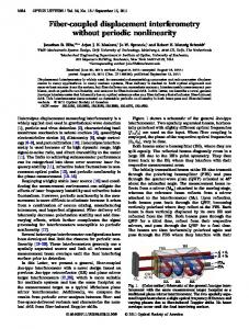
N(u,v) ˆ where N(u, v) = |N(u,v)| . A two dimensional example of a displacement map is shown in Figure 1, where N0 (u, v) is the normal to the displaced surface. ∗
[email protected] 1A
bivariate vector function is a function of two variables where the result is a vector.
1
GDC2003
P’ N’ D P N
Figure 1: Displacement mapping
2
DirectX 9.0 displacement mapping
The first API support for displacement mapping appears in DirectX 9.0. DirectX 9.0 supports two styles of displacement mapping, presampled and filtered. The presampled method is supported by ATI RADEON 9700 class hardware and filtered version by MATROX’s Parhelia hardware.
2.1
Presampled
Presampled displacement mapping allows the user to specify the values that are used at each vertex for displacement. An NPatch surface is used as the base surface. Depending on the level of detail set for NPatch tessellation, the number of vertices will be larger after tessellation. This increase from tessellation must be taken into account when generating the number of per vertex displacement values stored in the presampled set of displacement values. The total number of displacement values used is the sum of the input number of vertices plus the number of introduced vertices from tessellation. The one dimensional displacement map assigned to the vertex shader must contain the same number of presampled displacement values. As each vertex is passed into the vertex shader a displacement value is loaded into a register from the displacement map which has been set as a texture map for sampling. To displace a vertex along the normal the displacement value is loaded into a register and used to compute a new vertex position in the vertex shader.
2.2
Filtered
Filtered displacement mapping allows the user to specify a mipmap chain of displacement maps and sample them using tri-linear filtering. Using each vertex’s 2D texture coordinate, the appropriate mipmap level of the displacement map mipmap chain is bilinearly sampled based on the requied level of detail. The sampled value is placed in a register for use by the vertex shader to compute the displacement at that vertex in the same manner as that for the presampled case. The displacement map can be stored as 8bit or 16bit values.
2
GDC2003
Figure 2: The Crater Lake
3
Adaptive tessellation algorithms
Fixed tessellation inserts a fixed number of vertices into each triangle in a mesh regardless of whether the new vertices change the shape of the original triangle or are even visible within a particular rendering of the scene. Different schemes for adaptive tessellation for displacement mapping have been presented taking into account the change in the surface represented by the displacement map and screen size. A scheme using a series of tests for recursive adaptive tessellation was presented by Doggett and Hirche[3]. This scheme uses only edge based tests removing the need for global mesh information and allowing it to be implemented within the per triangle constraints of modern graphics hardware pipelines. Edge based tests also ensure that no cracking occurs when two triangles sharing the same edge introduce different tessellation levels. The edge based tests start by calculating a mid point for each edge. The first two tests are aimed at measuring the change in the curvature defined by the displacement map. Firstly the sum of displacements around the two end points and midpoint are found using a precomputed Summed-Area Table[2]. This detects any major changes in the average height surrounding each vertex. Using the summed heights around the vertex ensures that changes in height that are not located exactly at the vertices are detected. The problem with this test is that it averages the displacement values resulting in high frequency changes in the surface being missed if there is no low frequency change. To detect the low frequency change in surface curvature the normals at the two end points are compared with the new midpoint normal. Together these two simple tests detect the changes in the displacement map. Adapting tessellation level to view point is also important and this is performed by checking the pixel length of the edge in screen space. This test needs to be performed after the points are transformed into screen space. A final test is added to check that recursive tessellation is stopped once the resolution of the displacement map is reached. An example using this adaptive displacement mapping algorithm is shown in Figure 2. A similar recursive adaptive scheme is presented by Moule and McCool[9], which improves upon the robustness of the previous algorithm by using interval analysis. By
3
GDC2003
storing the minimum and maximum value in a mipmap chain, an interval that bounds an edge can be found. The naive approach would be to use the level of the interval heirarchy that bounds the desired edge, but this approach produces poor results. Instead they propose to use the union of up to four entries from the heirarchy to construct a tighter bound. This interval is compared against a threshold in screen space and if larger the edge is split. By comparing in screen space a view dependent tessellation is achieved. The combined coverage of the interval bounds on each edge of a triangle cover the entire area of the triangle. This ensures that all displacements across the surface of the triangle are taken into account. The tessellation scheme runs in real time without hardware support and is improved by preserving the results of the oracle between tessellation levels.
4
Other algorithms
Doggett, Kugler and Strasser [4] present a rasterization approach to displacement mapping where tessellation is driven by rasterization of the original triangle at an appropriate level of detail. A similar approach to using rasterization is also presented in [5], including the proposal to use the maximum height for generation of displacement map mipmap chains. Lee et al. [8] combine subdivision surfaces with displacement maps to create a surface representation that can adaptively select the level of detail by using only subdivision and bump maps, or add increasing amounts of detail by displacement mapping a subdivision surface. A volume rendering technique presented by Kautz[7] extrudes a volume along the normals of each triangle that contain the maximum extent of the displacement map. The volume is rendered using the typical hardware accelerated algorithm for volume rendering where transparent slices perpendicular to the view point are rendered. This technique requires high fill rates and large texture bandwidths. Techniques for ray tracing displacement maps are presented by Phar[10] and Heidrich[6].
References [1] Robert L. Cook. Shade Trees. Computer Graphics (Proceedings of SIGGRAPH 84), 18(3):223–231, July 1984. Held in Minneapolis, Minnesota. [2] Franklin C. Crow. Summed-Area Tables for Texture Mapping. Computer Graphics (Proceedings of SIGGRAPH 84), 18(3):207–212, July 1984. Held in Minneapolis, Minnesota. [3] Michael Doggett and Johannes Hirche. Adaptive view dependent tessellation of displacement maps. In SIGGRAPH/Eurographics Workshop on Graphics Hardware, pages 59–66, August 2000. [4] Michael Doggett, Anders Kugler, and Wolfgang Straßer. Displacement Mapping using Scan Conversion Hardware Architectures. Computer Graphics Forum, 20(1):13–26, March 2001. 4
GDC2003
[5] Stefan Gumhold and Tobias H¨uttner. Multiresolution rendering with displacement mapping. In Eurographics/SIGGRAPH Workshop on Graphics Hardware, pages 55–66, August 1999. [6] Wolfgang Heidrich and Hans-Peter Seidel. Ray-tracing procedural displacement shaders. In Graphics Interface, pages 8–16, 1998. [7] Jan Kautz and Hans-Peter Seidel. Hardware accelerated displacement mapping for image based rendering. In Graphics Interface, pages 61–70, June 2001. [8] Aaron Lee, Henry Moreton, and Hugues Hoppe. Displaced subdivision surfaces. In Computer Graphics, Proc. of SIGGRAPH 2000. ACM, 2000. [9] Kevin Moule and Michael D. McCool. Efficient bounded adaptive tessellation of displacement maps. In Graphics Interface, 2002. [10] Matt Pharr and Pat Hanrahan. Geometry caching for ray-tracing displacement maps. In Eurographics Workshop on Rendering, June 1996.
5
GDC 2003 Displacement Mapping Tom Forsyth, Muckyfoot Productions
[email protected] - www.muckyfoot.com January 12th, 2003
Principles Displacement Mapping is essentially a method of geometry compression. A low-polygon base mesh is tessellated in some way. The vertices created by this tessellation are then displaced along a vector usually the normal of the vertex. The distance they are displaced is looked up in a 2D map called a displacement map. The various hardware implementations have been well covered by Michael Doggett in his part of the talk, so I won’t go into details about those here. The main aim of this talk is to allow people to take what the industry’s current mesh and texture authoring pipelines produce, and to derive displacement map data from them. There will also be some discussion of rendering techniques on past, current and future hardware. It is worth mentioning that the problems and restrictions inherent in authoring for displacement maps are the same as the ones that occur when authoring for normal maps, because they are essentially two different representations of the same thing. Generating normal maps has recently come into fashion, and there is plenty of hardware around to support it. If you are going to be generating normal maps, it is almost certain that generating and using displacement map data is a relatively simple enhancement to the tool chain and rendering pipeline. As will be shown, there is similar widespread hardware support for at least some form of displacement mapping, and no doubt more on the way shortly.
Advantages Using displacement maps reduces the amount of memory required for a given mesh level of detail. Bulky vertex data is replaced by a 2D array of displacements – typically 8 or 16 bits in size, with most attributes such as texture positions, tangent vectors and animation weights implicit. This reduces storage requirements and the bandwidth needed to send that data to the rendering hardware, both of which are major limits on today’s platforms. Alternatively, it allows much higher detail meshes to be stored or rendered in the same amount of space or bandwidth. Reducing the mesh to a far simpler version (typically around a few hundred vertices rather than tens of thousands) means operations such as animation and morphing are cheaper. They can therefore be moved from the GPU back onto the CPU, which is a much more general-purpose processor. Because of this, the range of possible operations is expanded – more complex animations are possible and different techniques used, such as volume-preservation and cloth simulation. One other advantage is that the animation algorithms used are no longer tied to the specific GPU platform, or to the lowest-commondenominator of platforms – and indeed the animation programmer no longer needs to know the core details of the graphics platform to experiment and implement new techniques. A more general advantage is that using displacement maps turns meshes – tricky 3D entities with complex connectivity – into a few 2D entities. 2D objects (i.e. textures and images) have been studied extensively, and there are a lot of existing techniques that can now be applied to meshes. For example: • Mesh simplification becomes mipmap generation. • Compression can use JPEG-style or wavelet-based methods. • Procedural generation of meshes can use existing 2D fractal techniques. • Morphing becomes a matter of blending 2D images together. • End-user customisation involves 2D greyscale images, rather than complex meshes. Using graphics hardware and render-to-texture techniques, many of the above features can be further accelerated.
Disadvantages Displacement maps place some restrictions on the meshes that can be authored, and are not applicable everywhere. Highly angular, smooth or faceted objects do not have much fine or complex surface detail, and are better represented either by standard polygonal mesh data, or by some sort of curved surface representation such as the Bezier family of curves, or subdivision surfaces. Highly crinkled or fractal data such as trees or other plants are not easy to represent using displacement maps, since there is no good 2D parameterisation to use over their surfaces. Then again,
no other current rendering technology except volumetric representations works well for this style of objects. Meshes that overlap closely or have folds in them can be a problem, such as collars or cuffs or layers of material such as jackets over shirts, or particularly baggy bits of material. This is because a displacement map can only hold a single height value. Although this is a problem at first, if artists can author or change the mapping of displacement maps, they quickly learn to map each layer to a different part of the displacement map, and to duplicate each layer in the low-polygon base mesh. Automated tools are also easy to modify to do this correctly. Authoring displacement maps almost always requires specialised tools – it is very hard to directly author the sort of maps discussed here (large-scale ones that cover a whole object). However, the amount of work required to write or buy these tools is small compared to the benefits. The required or recommended tools are discussed below. At first glance, hardware support is very slim for displacement mapping. Currently, only two PC graphics cards support it natively (the Parhelia and the Radeon 9700), and none of the consoles. However, with a bit of thought, displacement mapping methods can be applied to a much wider range of hardware. On the PC, anything using any sort of vertex shader can use them, including software VS pipelines used by many people for animation or bump-mapping on older cards. On the consoles, the VU units of the PS2 can use displacement maps directly, and any CPU with a SIMD instruction set (such as the GameCube’s) can efficiently render displacement map data. On the consoles, the reduction in memory use and memory bandwidth is well worth the extra effort.
Required Source Data To use displacement mapping in hardware or software, you eventually need the basic ingredients: • A heightfield displacement map, for displacement of vertices. • A normal map, for lighting. • A low-polygon base mesh. • A texture mapping for the displacement and normal maps over the base mesh. Typically, displacement maps are lower-resolution than normal maps, though they may demand more precision. Additionally, displacement maps and normal maps usually share the same mapping, since the same problems must be solved by both – filtering (especially mipmapping), representation of discontinuities, texel resolution at appropriate places on a mesh, and so on. How you get these basic ingredients is almost entirely up to the art team and the available tools. They are available from many sources in many combinations. For reference, all vertex numbers given are for a human figure that would normally take around 10,000 vertices to represent with a raw mesh, with around 40 bones. Typically, there are twice as many triangles as vertices in a mesh.
Low-Polygon Base Mesh As a guide, this mesh is around 100 vertices for a human figure, depending on the quality of animation required and the complexity of their clothing. The artists can directly author this, or it can be derived from higher-polygon meshes by using a variety of techniques. Some of these may be completely automatic, or they may be semi-automatic, with visual checks and tweaks by artists. There are many methods to automatically reduce meshes in complexity. Edge-collapse based ones are popular, especially as they can also be used to directly author Progressive Mesh sequences, which are useful for rendering continuous levels of detail. Using Delaunay-style parameterisation and remeshing is also an option.
Unique Texture Mapping Displacement and normal maps generally require a mapping over the mesh that ensures that each texel is used no more than once. Although not strictly necessary in some specialised cases (for example, when an object has perfect left/right symmetry), in general the extra flexibility is well worth the effort. The unique mapping can be authored directly, using a spare mapping channel in the mesh. Automated generation is possible using the same Delaunay-style parameterisation as the above remeshing, or using the technique in Gu et al’s Geometry Images1 of a minimal number of cuts to unfold a mesh onto a flat square plane. There are also existing unique mapping solutions in 3D authoring tools, such as 3DSMax’s “flatten” mapping – these are adequate for quick prototypes, but tend to
introduce a lot of unwanted discontinuities, which hinder many of the polygon-reduction techniques used to produce the low-polygon base mesh. The unique mapping can also be used for lightmap generation or procedural textures, if applicable.
Heightfield Displacement Map and Normal Map Displacement maps can be authored directly using greyscale textures and suitable art tools. However, 8 bits per pixel is generally not sufficient for a full displacement map, and few if any art packages handle 16 bit greyscales. Even when they do, since they are designed for visual use rather than heightfield authoring, the control over them is relatively coarse, and it is hard for artists to achieve anything but an approximation of the correct shape. In practice, this leads to “caricatures” of what is desired. A better choice is to author most or all of the data using a high-polygon mesh. Using the unique mapping above, each texel on the displacement and normal maps has a single position on the lowpolygon base mesh. A ray is cast from that position along the interpolated normal, and the intersection with the high-polygon mesh is found. The normal of the high-polygon mesh is written into the normal map, and the distance along the ray to the point of intersection is written into the displacement map. When authoring the high-polygon mesh, the artists do still need to be aware that they are indirectly authoring a heightfield. Folding or overlaps of geometry will not be recorded well by a heightfield. In practice, we find it is better to have the ray-caster report difficult or ambiguous intersection cases and have the artists fix up the mesh (either the high or low-polygon ones as appropriate), than to attempt to make the ray-caster very intelligent. These tricky cases are rare, and this method highlights them, reducing unwanted surprises. Normal maps (either object-space or surface-local space) are almost impossible to author directly, but are easily generated from displacement maps or “bumpmaps”. Although a bumpmap is actually a form of heightfield, since absolute scale is far less important when generating normal maps than with displacement maps, they are routinely generated by hand. High-frequency displacement and normal maps are fairly easy to author. These are used to provide texture to a surface, or to add small ridges or creases. These are often applied to medium-polygon meshes to add fine details, rather than to the low-polygon mesh that is used in displacement mapping. It is easy to apply them to existing or generated displacement and normal maps as long as there is already a unique texture mapping. The high frequency implies small displacements, so the lack of a wellcontrolled scale for those displacements is not as much of a problem. Having a crease in clothing twice as large as desired is not a major problem, unlike having a character’s nose twice as long as it should be. Note that the mapping of these high-frequency maps is still flexible, and it is perfectly acceptable to tile a small texture over a larger surface to provide noise and detail. They will be rendered into the normal and displacement maps, and it is those that are uniquely mapped.
Muckyfoot Choices At Muckyfoot we tend to author medium-polygon meshes (around the 3,000 mark for humans) with high-frequency bumpmaps. It is more efficient to put small creases and surface texture into a bumpmap than it is to generate them with polygonal creases, and just as visually effective. It also reduces the problem of high-frequency polygon data confusing the ray-caster and causing multiple intersections. We author the unique mappings directly, and they are usually relatively quick for artists to generate using existing mapping tools. The additional control compared to automated mapping is well worth the time, since this is an area that computers seem to be particularly poor at compared to humans, and humans can make far better judgements over perceptual importance and allocate more or less texture space accordingly. Additional improvements are mentioned below in the “tools” section that make this process easier and quicker. Typical mapping time for a human mesh is around two hours, though the mapping on many different humans is virtually identical, so the effort is amortised over many meshes. To produce a low-polygon base mesh, Muckyfoot use a Quadric Error Metric-based semi-automatic edge-collapse sequence that is visually checked and manually tweaked where necessary. Fully automated reduction is generally acceptable down to around 500 vertices, and then manual tweaking can be required in around 10 places to reduce to 100 vertices. The tweaking is generally required to collapse features that are visually unimportant such as the feet, or to prevent collapse of perceptually important features such as the face, elbows, knees and hands. Automation of these (for example, taking bone weights into account) was attempted with mixed results – it seems generally quicker and better simply to allow the artists full control by this stage – frequently the extra “intelligence” of the tool gets in the way. Production of a low-polygon mesh typically takes around 30 minutes per human mesh, which compares well with the initial authoring time.
As well as producing the low-polygon base mesh, this process also generates a View Independent Progressive Mesh, which is useful when rendering the mesh on some hardware (see below). The same tool also produces VIPM sequences for objects that do not use displacement maps - simple or smooth objects such as coffee mugs, dustbins, chairs and desks. The high or mid-polygon meshes that the artists author are only used as input to the offline ray-caster – they are not used directly at runtime. Because of this, the limits imposed by the rendering pipeline on polygon counts are almost totally removed. The new limit on polygon count is simply whatever the artists have time to author. The limits on connectivity, large or small polygon sizes, and mesh complexity are also largely removed (as long as a sensible low-polygon base mesh can be produced). Games are getting bigger, and more and more limited by what we have time, talent and manpower to author, rather than by the hardware, and this extra flexibility allows the artists to optimise for their time, rather than for the peculiarities of a graphics engine.
Art Tools We found a number of tools handy when authoring displacement maps. A lot of these tools have other uses, such as the QEM-based edge collapser which also generates View-Independent Progressive Mesh data. Some of them already exist in various forms, and experimenting with these off-the-shelf solutions is a very good idea before committing to writing custom tools.
Displacement Map Previewer If displacement maps are authored directly, some sort of preview tool is usually needed. Some 3D packages may have displacement map renderers included, but if not it is fairly simple to write a bruteforce previewer that simply tessellates the base mesh to the resolution of the displacement map – one quad per texel. Although it is a lot of triangles to draw, if done on a single object at a time, it is not unreasonable. A 512x512 map requires half a million triangles to render, which can be rendered at acceptable speeds on a decent PC graphics card. If displacement maps are extracted from a high-polygon mesh, this previewer is usually not necessary.
Unique Mapping Checker When creating unique texture mappings, it is easy for a machine or artist to accidentally map two areas of mesh to the same bit of texture. This is easily solved by rendering the mesh to a texture using the UV mapping as XY co-ordinates, counting each time a particular texel is touched. Where a texel is touched more than once, render an opaque red texel. Otherwise, render a translucent blue texel. When the mesh is loaded back into a 3D modelling package and the texture applied to it, any red/opaque texels show where the problem spots are, and of course there will be red texels in both the places that conflict, making it easy to spot and correct the overlap. This tool is usually a special mode of the ray-caster, since both rasterise base-mesh polygons onto a uniquely mapped texture. The difference is that the ray-caster does a lot more work to decide what data to write to the texels.
Ray-caster The ray-caster rasterises base-mesh triangles to the displacement and normal maps. For each texel, it casts a ray from the texel’s position on the base mesh (after interpolation by whatever basis is used – linear, N-Patches, subdivision surfaces, etc) along the normal, looking for the best intersection with the high-polygon mesh. “Best” is defined by various heuristics. It is usually the nearest intersection to the base mesh, though if multiple intersections are close together, this often indicates a high-frequency part of the mesh that folds back on itself, or a mesh “decal” where smaller polygonal details have been added over a coarser part of the mesh. Usually, the furthest of these bunched intersections is used. The ray-caster takes the normal of the high-polygon mesh, modifies it by any applied bumpmap and writes it to the normal map. It takes the distance along the ray from the base mesh to the intersection and writes that value into the displacement map. Any high-frequency bumpmap applied to the high-polygon mesh will also modify the displacement at this stage as a “detail” displacement map. In theory a bumpmap should perturb the high-polygon mesh and alter where the ray intersects it. However, we have found that simply adding the bumpmap height onto the intersection distance produces perfectly acceptable results as long as the bumpmap has a small displacement scale, and is only used for creases and small bumps, rather than major features.
After the ray-caster has written texel data to the normal and displacement maps, the maps are usually sent through a dilation filter, which spreads written values outwards to any neighbouring unwritten texels. This fills in the gaps between mapped areas with sensible data, and ensures that filtering still brings in sensible data, especially when mipmapping. ATI’s “Normal Mapper”2 and Crytek’s “PolyBump”3 both do this ray-casting, though at the time of writing both only output normal maps. It would be simple to modify them to output displacement data as well. Both include a variety of heuristics to decide the “best” intersection to use for various cases.
Unique Mapping Packer There are two problems in unique mapping. One is to get a unique mapping so that no texel is used in two places, and the other is to pack the many small areas of connected triangle “patches” together in the most efficient way. The first part can be solved by automation, but humans seem to do equivalently well in the simple cases and a far better job in the tricky cases. The second part – equivalent to the problem of packing odd shapes in a box – is tedious for humans. But because it involves no perceptive judgement calls, it is simple to leave a computer crunching away through possible solutions (possibly overnight) until it finds a good one. To reduce “bleeding” between patches due to filtering (especially mipmapping), patches must be separated by certain minimum numbers of texels. After packing, these texels are filled with the value of the nearest used texel, again so that filtering does not bring in undefined values. This automatic packing allows artists to concentrate on the tricky task of uniquely-mapping an object. They do not have to simultaneously keep all the bits optimally packed – they can scatter them all over the UV domain and arrange them for easier mental labelling (all the parts of one type together, etc). A further enhancement is to analyse the frequency of the displacement and normal map data in each triangle patch and scale them up or down to allocate more texture space to the areas with the higherfrequency data. By packing the patches together after this scaling, a given size of displacement or normal map will be spread over the object with more texels applied to detailed areas. It is important not to completely remove the artist-determined scales. A maximum grow/shrink factor of two in each UV axis is sufficient to ensure good use of available space, but allows artists to deliberately allocate extra texel space to areas of high importance, such as the face and hands of people, and reduce perceptually minor parts such as the undersides of cars, which are very crinkly, but not very visible (unless it’s that sort of game of course!) Note that this scaling implies a slightly more complex pipeline. First the patches are packed together without scaling – this is just to get them all onto a single map of reasonable size – the packing does not need to be very efficient. Then the ray-caster is run to produce a first approximation of the displacement and normal map data. For quick previews, that data is then used directly for display. For final artwork, the frequency of the data in each patch is determined, and the patches are scaled accordingly and repacked with a more expensive algorithm. Then the ray-caster is run again with this new optimal mapping, usually with a very high-resolution map. The large map is then filtered down to the actual size stored on disk. This second pass is typically run on a batch job overnight, which means it can devote a lot of time to finding near-optimal packing, and use really big maps for the ray-casting phase, removing as many sampling artefacts as possible. Alternative methods of optimising texture space for signal frequency are given by Sander et al4.
Mesh Reduction Probably the trickiest tool to get right, since it usually needs to have an interactive element to it, and because it relies on a lot of heuristics. The commonest mesh-reduction techniques are based on incremental edge collapses. This technique produces a Progressive Mesh5 as it works, which can be used for rendering continuous level of detail meshes (discussed later on). Many heuristics exist to decide the order of edge collapses, most based on the Quadric Error Metric by Garland and Heckbert6 or modifications of it by Hoppe7. These are the style of Progressive Meshes generated by the Direct3DX library, and the low-polygon data it outputs can be used directly as the base mesh. Alternatively, there are various styles of re-meshing using Delaunay triangulation8
Rendering Once the basic data of a low-polygon mesh, a displacement map, a normal map, and a mapping for the maps is obtained, the data can be processed for the capabilities of the target hardware. Much of the details are either proprietary (in the case of consoles) or have been discussed elsewhere (in the case of
my “Displacement Compression” techniques9), so only brief outlines are given here. This processing rarely requires any human intervention fortunately, and is fairly simple number-crunching. I shall address each platform separately. The techniques for rendering normal maps are fairly standard between most of these platforms. The exception (as always) is the PlayStation2, but again these details are proprietary.
Adaptive Displacement Mapping • Matrox Parhelia; future hardware. Make mipmaps of the displacement map, and render the low-polygon mesh with the displacement map. If necessary, feed some distance-related or perceptual biases into the adaptive tessellator. The hardware does the rest.
Pre-sampled Displacement Mapping • ATI Radeon 9700; maybe PlayStation 2. Regularly and uniformly tessellate the base mesh in software and sample the displacement map at the generated vertices. This produces an array of n(n+1)/2 displacements for each triangle on the base mesh. These values are swizzled in a hardware-specified manner into a stream fed to the vertex shader. To perform Level of Detail transitions, repeat the above process for a variety of different tessellation amounts (generally the powers of two), giving an effective “mipmap chain” of displacement streams. This allows discrete LoD transitions, though with some popping as the mesh switches from one tessellation level to the next. To remove the popping, each displacement stream entry holds two displacements rather than one. The first holds the standard displacements, and the second holds the up-sampled displacements from the lower-LoD tessellation. In the vertex shader (or equivalent), a per-mesh global interpolates between the two sets of displacements. Just using these up-sampled values should give a mesh that is visually identical to the lower LoD version. As an object goes away from the camera, this allows the high LoD version to smoothly morph into the low LoD version, and then the low LoD version swapped in with no visual popping, but reducing the triangle and vertex count. Because this method samples the displacement map in a predictable manner, you may get some improvement in quality by ray-casting at the required positions directly rather than going via a displacement map. This also means that a unique mapping is not required for displacements, since there is no actual 2D displacement map, simply a displacement stream for each triangle of the base mesh. However, a unique mapping is still required for the normal map. The Radeon 9700 is the only current card to explicitly support this method, though it seems possible that the PlayStation2 could also implement it with a bit of work. As with all things on the PS2, it depends heavily on the rest of the rendering pipeline being used.
Displacement Compression •
nVidia GeForce 3 and above; ATI Radeon 8500; GameCube; XBox; PlayStation 2; software Vertex Shader pipelines on DX6 or better cards. The base mesh vertices are uploaded to the memory of the vertex unit, rather than in a standard mesh/vertex stream. This may need to be done in multiple sections because of limited vertex unit memory, with each section drawn before the next is uploaded. Tessellation of the mesh is performed offline to whatever degree required, and the tessellated vertices and/or indices fed in as a standard mesh. The difference is that rather than holding raw vertex position, normal, texture co-ordinates, etc, each vertex stores only the following data: • Three indices to three base-mesh vertices. • Two barycentric co-ordinates that interpolate between the base-mesh vertices. • A displacement value. This reduces the size of a vertex to 6 bytes (though many systems require padding of the vertices up to 8 bytes). The vertex unit interpolates position, normal, texture co-ordinates, tangent vectors and so on from the given three base-mesh vertices and the two barycentric coordinates. The vertex is then displaced along the interpolated normal. Interpolation can be performed using any basis, but linear and bicubic are common. Linear interpolation is fine for most objects, though highly-animated objects may benefit from using an NPatch-style basis because it is relatively smooth even under heavy mesh distortion. As with pre-sampled displacement mapping, there is no actual 2D displacement map, so the displacement for each vertex can be sampled directly using the ray-caster if desired.
Level of detail transitions can be done using the same trick as with pre-sampled displacement mapping – storing two displacements per vertex and lerping between them – or using ViewIndependent Progressive Meshes. Muckyfoot currently uses the lerping method on the PlayStation2, and on other platforms with indexed primitive support, we use “sliding window” VIPM10. It is possible to reformulate this method so that instead of sending base-mesh vertices to the vertex unit, base-mesh triangles are sent. Each displaced vertex then only needs a single index to determine which triangle it is on. This reduces the possible size of vertices down to 4 bytes. However, since there are typically more triangles then vertices in the base mesh, and more information is required to store a triangle, and vertex unit storage space is typically at a premium, this may be slower except for highlytessellated objects with simple base meshes.
Start-of-Day Tessellation •
Slow CPUs with DX5 or earlier graphics cards; software rasterisers; laptops; PDAs; mobile phones. These devices do not have enough polygon throughput and/or CPU power to use runtime displacement mapping to any useful extent. However, you can tessellate and displace the data using software either at installation time or at start of day. By tessellating according to the measured CPU speed of the machine, and tessellating multiple versions of each mesh, you still gain the advantages of adapting polygon count to the scene complexity, machine capability and the size of each mesh on the screen without having to author them directly. If the data is delivered on a format with reduced bandwidth or size – for example over a modem or on a multi-game “sampler” disk, you gain the excellent compression and space savings that come with using displacement and normal maps. On really slow hardware, the low-polygon base map is just used directly with no tessellation at all. Some software rasterisers may be able to do normal mapping, and some hardware may be able to use the displacement map data to do emboss bumpmapping. Otherwise, it is easy to do a pre-lighting phase applied to the normal map with the mesh in its default pose and light coming from above, to give lights and shadows in appropriate places. While not strictly correct, it produces images easily acceptable by the standards of the available hardware, but does not cost any extra authoring time to produce.
Summary Displacement mapping reduces memory use and increases mesh detail. Once displacement maps are authored, highly scalable content is easy to generate automatically, allowing an application to use very long view distances, more complex scenes, a wide variety of platforms, and to an extent future-proof itself and the art assets for future hardware. The difficulties of authoring displacement maps directly are reduced to a far more manageable pipeline with a few simple tools and a small amount of artist training. Previously, greater effort was frequently expended authoring and re-authoring different levels of detail for different platforms, or to rebalance processing load for specific scenes. Almost all of the difficulties with displacement maps are shared by the generation of normal maps – if generating one you can frequently get the other with very little effort. Despite appearances, there is already wide hardware support for displacement maps – all the current consoles and almost all “gamer” PC hardware. Newer hardware allows more efficient implementations of displacement mapping, but any of the methods listed gives speed and size advantages over raw mesh rendering. 1
“Geometry images.” X. Gu, S. Gortler, H. Hoppe. ACM SIGGRAPH 2002, pages 355-361 ATI Normal Mapper tool, available from http://mirror.ati.com/developer/index.html 3 Crytek PolyBump package - http://www.crytek.com/ 4 “Signal-specialized parametrization.” P. Sander, S. Gortler, J. Snyder, H. Hoppe. Eurographics Workshop on Rendering 2002. http://research.microsoft.com/~hoppe/ 5 “Progressive meshes.” H. Hoppe. ACM SIGGRAPH 1996, pages 99-108 6 “Surface simplification using quadric error metrics.” M. Garland,P. Heckbert. SIGGRAPH '97 Proceedings, Aug 1997 7 “New quadric metric for simplifying meshes with appearance attributes.” H. Hoppe. IEEE Visualization 1999, October 1999, pages 59-66 8 “Multiresolution analysis of arbitrary meshes.” M. Eck, T. DeRose, T. Duchamp, H. Hoppe, M. Lounsbery, W. Stuetzle. Computer Graphics 1995 2
9
Displacement compression presentations in Meltdown 2000 and 2001, T. Forsyth. Available from http://www.tomforsyth.pwp.blueyonder.co.uk/VIPM_papers.html 10 "Comparison of VIPM Methods." T. Forsyth. Games Programming Gems 2, Charles River Media 2001. ISBN 1584500549