M.C. Nichols, D.R. Boehme, R.W. Ryon, D. Wherry, B. Cross and G. Aden, ... B.J. Cross and D.C. Wherry, âX-ray Microfluorescence Analyzer for Multilayer Metal.
Copyright(C)JCPDS-International Centre for Diffraction Data 2000, Advances in X-ray Analysis, Vol.42
Copyright(C)JCPDS-International Centre for Diffraction Data 2000, Advances in X-ray Analysis, Vol.42
XRF MAPPING: NEW TOOLS FOR DISTRIBUTION ANALYSIS B. Scruggd, M. Haschke2, L. Herczeg’, J. Nicolosi’
‘Edax Inc; Mahwah, NJ 2RiintgenanalytikMeJtechnik GmbH; Taunusstein,Germany INTRODUCTION With the advent of x-ray micro-fluorescence (XMRF) technology some years ago (1,2,3,4), it has become feasible to map elemental distributions in samples (5,6, 7,s) using XRMF. Up to now, to the best of our knowledge, XRF mapping has been done by defining an elemental line or a region of interest (ROI) prior to data collection. This type of elemental distribution analysis is typically referred to as ROI mapping. Hence, in order to take full advantage of the energydispersive (ED) XRF technique, one must have an in-depth knowledge of all of the elements or regions of interest in a sample prior to mapping analysis. Without this knowledge, one must rely on mathematical analysis of the data to indicate where x-ray counts are deficient in the distribution map, add missing elements to the distribution analysis and reacquire the data. This approach forfeits the ED-XRF advantage to collect a full energy spectrum. To overcome this problem, we introduce the concept of Spectral Mapping for XRF elemental distribution analysis. Spectral Mapping has been used previously for distribution analysis using scanning electron microscopy-energy dispersive spectroscopy (SEM-EDS) (9). Spectral Mapping allows for the collection of a full XRF spectrum at each map pixel. Hence, when an elemental distribution analysis is found to be lacking certain elements, the spectral map data can be reprocessed to add to the distribution analysis. The actual data does not have to be collected a second time. EXPERIMENTAL Mapping data was acquired using the Edax Eagle u-Probe XRMF spectrometer. The spectrometer was equipped with a Rh micro-focus tube and 300 urn mono-capillary. The system has a 40 W maximum power output with a 40 kV maximum. The x-ray focal point is nominally 10 mm from the capillary tip. Edax Spectral Mapping and advanced image processing (IDX) software was used for this demonstration. The sample was a piece of sandstone known, prior to data collection, to contain particles of sodium feldspar (or “albite”) and quartz bound together with calcium carbonate cement (see Figure 1).
19
19
Copyright(C)JCPDS-International Centre for Diffraction Data 2000, Advances in X-ray Analysis, Vol.42
Copyright(C)JCPDS-International Centre for Diffraction Data 2000, Advances in X-ray Analysis, Vol.42
Figure 1: Video image from the Eagle p-Probe of a piece of polished sandstone embedded in epoxy. Since the sandstone was originally prepared for SEM-EDS analysis, the sandstone is embedded in epoxy and polished; however this is not necessary for XRMF analysis. The analyzed area is approximately 10 mm by 13 mm. RESULTS AND DISCUSSION From the initial information known, Na, Ca and Si would be elements chosen for ROI mapping analysis. In Figure 2, the Na, Ca and Si distribution analysis of the sandstone is shown.
A: NaKMap
B: SiKMap
I
C: CaKMap
m D: Gveriay Map: Na, Si, Ca
Figure 2: Sandstone elemental distribution analysis (nominal 13 mm by 10 mm area) assuming Na, Si and Ca elements in the distribution. In the overlay map (D), holes in the map, shown by asterisks, indicate missing data.
20
20
Copyright(C)JCPDS-International Centre for Diffraction Data 2000, Advances in X-ray Analysis, Vol.42
Copyright(C)JCPDS-International Centre for Diffraction Data 2000, Advances in X-ray Analysis, Vol.42
Mapping data was collected under the following conditions: 20 kV 128 x 100 pixels Dwell time/pixel = 5 s Total acquisition time - 18 hrs Data collection was not optimized with respect to total time of acquisition. For example, while degrading the visual quality of the images somewhat, a 64x50 pixel map would contain the same information (only a 43x33 pixel map is required to cover the analyzed area) with a factor of 4 reduction in total acquisition time. For an experienced geologist, the elements selected for analysis in Figure 2 may not be the only logical choices. But this requires the availability of someone with an in-depth knowledge of the sample or class of materials studied. In a normal ROI mapping analysis, the deficient areas in the overlay map would have to be re-examined via XRMF to identify missing elements in the initial ROI distribution analysis. The distribution analysis would then have to be re-collected. To avoid this rather problematic process, the idea to collect all of the information available at each map pixel, spectral mapping, which utilizes the full power of ED-XRF was conceived.
Spectral Mapping Spectral mapping software allows the user to collect a full XRF spectrum at each map pixel. Each spectrum is then correlated to a specific position. Currently, the spectral map data can be searched in a number of simple ways: l
l
l
Each spectrum per pixel: the spectrum from each map pixel can be displayed by mouseclicking on a pixel of interest in the video image. Summed spectrum: spectra closest to a line or within a boxed area defined in the video image can be summed and displayed. Total map spectrum: all of the spectra in the map can be summed and displayed. (see Figure 3)
21
21
Copyright(C)JCPDS-International Centre for Diffraction Data 2000, Advances in X-ray Analysis, Vol.42
Copyright(C)JCPDS-International Centre for Diffraction Data 2000, Advances in X-ray Analysis, Vol.42
Magnesium
Potassium
Iron
Figure 3: Total map spectrum of Sandstone. Elements previously “unknown” in the distribution analysis include magnesium, potassium and iron. In this particular case, the total map spectrum shown in Figure 3 revealed additional elements not included in the preliminary ROI mapping analysis. Among other peaks, magnesium, potassium and iron can be readily identified. Re-evaluating the spectral data for magnesium and iron, it can be seen that these elements are primarily associated with the calcium carbonate cement bonding the sandstone mineral particles together (see Figure 4).
B: FeMap
A: CaMap
C: Mg Map Figure 4: Sandstone spectral mapping data (nominal 13 mm by 10 mm area) reprocessed to display Fe and Mg distribution maps.
22
22
Copyright(C)JCPDS-International Centre for Diffraction Data 2000, Advances in X-ray Analysis, Vol.42
Copyright(C)JCPDS-International Centre for Diffraction Data 2000, Advances in X-ray Analysis, Vol.42
Reprocessing the spectral map data for the potassium map clearly shows that potassium completes the primary distribution analysis of the sandstone (see Figure 5).
A: Overlay: Na, Si, Ca
C: OvtllaJ.
IT=, Si, Ca, K
B: K Map Figure 5: Combination of the Na, Si, Ca Overlay map (nominal 13 mm by 10 mm area) with the K map reprocessed after data acquisition. Na (green); Si (blue); Ca (red); K (cyan) Diffraction peaks are a common phenomenon in ED-XRF spectra. An ED-XRF spectrometer for bulk-area or micro-area analysis has a fixed geometry between the x-ray tube, the sample and the x-ray detector. It is therefore possible for incident x-rays to diffract from crystal planes within the sample into the detector. Diffraction occurs when x-rays of a particular energy impinge upon crystal planes at a particular orientation such that Bragg’s law is satisfied. Diffraction peaks are typically identified by: (1.) changing the orientation of the sample (The energy of a single diffraction peak is a function of sample orientation.); (2.) comparing peak width to typical detector resolution at that energy (Diffraction peaks are broader in comparison to elemental lines.); (3.) identifying the presence of complimentary x-ray peaks within an elemental series. However, without a detailed crystallographic study of the sample, it is not possible to predict where the diffraction peaks from a sample will appear in the ED-XRF spectrum. Therefore, ROT mapping of diffraction peaks can only be accomplished after a detailed XMRF study of the sample. But with spectral mapping, diffraction peaks can be identified with the tools previously described and mapped without reacquiring data. In Figure 6, an example of the use of spectral mapping to search for and map a diffraction peak is given, The spectra associated with the boxed area on the sandstone image are summed together
23
23
Copyright(C)JCPDS-International Centre for Diffraction Data 2000, Advances in X-ray Analysis, Vol.42
Copyright(C)JCPDS-International Centre for Diffraction Data 2000, Advances in X-ray Analysis, Vol.42
Figure 6: The spectrum is the summation of all the spectra associated with the map pixels encompassed by the white box in the video image. A diffraction peak is found in this region of the spectral distribution analysis. in the figure. The predominance of the Si peak indicates that this region is primarily associated with quartz. Also, the summation spectrum from the boxed region shows a diffraction peak at 4.7 keV (10). Given the fixed geometry of the Eagle spectrometer, this diffraction peak correlates to oriented crystallites with a 2d lattice spacing of -2.84 A. In Figure 7, reprocessing the spectral map data with an ROI around 4.7 keV generates a map of these oriented crystallites.
Ca, K, DP (centroid - 4.7 keV) Figure 7: 4.7 keV Diffraction Peak (DP) map and overlay of DP map (nominal 13 mm by 10 mm area) on Sandstone elemental overlay map. Na (green); Si (blue); Ca (red); K (cyan); DP (yellow)
SUMMARY A new software tool for XRF elemental distribution analysis, spectral mapping, has been discussed. Spectral mapping can collect a full spectrum at each map pixel in the distribution and,
24
24
Copyright(C)JCPDS-International Centre for Diffraction Data 2000, Advances in X-ray Analysis, Vol.42
Copyright(C)JCPDS-International Centre for Diffraction Data 2000, Advances in X-ray Analysis, Vol.42
therefore, takes full advantage of the ED-XRF technique. This allows the user to collect the data only once and then reprocess the data for different elemental lines and ROI’s not included in the initial map data acquisition. The previous technique, ROI mapping, requires an in-depth knowledge of the sample, both composition and diffraction peak structure, to avoid having to repeat the distribution analysis.
REFERENCES
PI PI PI
M.M. Jaklevic, W.R. French, T.W. Clarkson and M.R. Greenwood, ‘“X-ray Fluorescence Analysis Applied to Small Samples”, A&. X-ray AnaZ.,21 (1978) 171-185. T.Y. Toribara, D.A. Jackson, W.R. French, A.C. Thompson and J.M. Jaklevic, ‘Nondestructive X-ray Fluorescence Spectrometry for Determination of Trace Elements Along a Single Strand of Hair”, Anal. Chem., 54 (1982) 1844- 1849. M.C. Nichols, D.R. Boehme, R.W. Ryon, D. Wherry, B. Cross and G. Aden, ‘Parameters Affecting X-ray Microfluorescence (XRMF) Analysis”, Adv. X-ray Anal., 30 (1987) 45-51.
PI [51
B.J. Cross and D.C. Wherry, “X-ray Microfluorescence Analyzer for Multilayer Metal Films”, Thin SoZ.Films, 166 (1988) 263-272. D. R. Boehme, “X-ray Microfluorescence of Geologic Materials”, A&. X-ray Anal., 30 (1987) 39-44.
Fl PI PI
D.A. Carpenter, M.A. Taylor and C. E. Holcombe, “‘Applications of Laboratory X-ray Microprobe to Materials Analysis”, 32 (1989) 115- 120. D.A. Carpenter and M.A. Taylor, “Fast, High-Resolution X-ray Microfluorescence Imaging”, 34 (1991) 217-221. J.A. Nicolosi, B. Scruggs and M. Haschke, “Analysis of Sub-mm Structures in Large Bulky Samples using Micro-X-ray Fluorescent Spectrometry”, Adv. X&y Anal., 41 (1998).
PI WI
Edax Product Profile, “Spectral Mapping”, (1997). M. ImatZu, “Development of Fast Texture Mapping System with Energy Dispersive X-ray Diffraction Method”, Ah. Xky Anal., 40 (1997).
25
25