Image Storage and Compression-Part 2. Thurman ... ing, and analyzing radiologic images on personal com- puters. ...... London, UK, Blenheim Online, 1990. 22.
Journal of Digital Imaging FEBRUARY 1994
VOL 7, NO 1
IMAGES ON PERSONAL COMPUTERS Displaying Radiologic Images on Personal Computers: Image Storage and Compression-Part 2 Thurman Gillespy III and Alan H. Rowberg This is part 2 of our article on image storage and compression, the third article of our series for radiologists and imaging scientists on displaying, manipulating, and analyzing radiologic images on personal computers. Image compression is classified as lossless (nondestructive) or lossy (destructive). Common lossless compression algorithms include variable-length bit codes (Huffman codes and variants), dictionarybased compression (Lempel-Ziv variants), and arithmetic coding. Huffman codes and the Lempel-ZivWelch (LZW) algorithm are commonly used for image compression. All of these compression methods are enhanced if the image has been transformed into a differential image based on a differential pulse-code modulation (DPCM) algorithm. The LZW compression after the DPCM image transformation performed the best on our example images, and performed almost as well as the best of the three commercial compression programs tested. Lossy compression techniques are capable of much higher data compression, but reduced image quality and compression artifacts may be noticeable. Lossy compression is comprised of three steps: transformation, quantization, and coding. Two commonly used transformation methods are the discrete cosine transformation and discrete wavelet transformation. In both methods, most of the image information is contained in a relatively few of the transformation coefficients. The quantization step reduces many of the lower order coefficients to 0, which greatly improves the efficiency of the coding (compression) step. In fractal-based image compression, image patterns are stored as equations that can be reconstructed at different levels of resolution. Copyright © 1994 by W.B. Saunders Company KEY WORDS: personal computer, image compression, differential pulse code modulation, Huffman codes, Lempel-Ziv-Welch compression, discrete cosine transformation, discrete wavelet transformation, fractal compression, tagged interchange file format.
PART 2 of our review article on and compression. Part 1 reT HISimageIS storage Journal of Digital/maging, Vol 7, No 1 (February), 1994: pp 1-12
viewed image storage and the fundamental principles of information theory and image compression. In this part, we review different methods of lossless and lossy image compression. This is the third article of our series for radiologists and imaging scientists on displaying, manipulating, and analyzing radiologic images on personal computers. LOSSLESS IMAGE COMPRESSION
Run-Length Encoding
The run-length encoding (RLE) compression algorithm replaces a sequence of pixels with the same value with an RLE code and the number of occurrences. For example, 20 consecutive zero-value pixels can be encoded by the sequence: (RLE code) (20). RLE is commonly used for bilevel or bit-mapped images in which long stretches of white and black pixels occur in series. This algorithm is not very useful for continuous-tone gray scale or color images, but is sometimes used in conjunction with other compression techniques. In addition, RLE may be useful for compressing the edges of radiologic images that are very dark (pixel values = 0) and do not contain any anatomically useful information.
From the Department of Radiology, University of Washington, Seattle, WA. Address reprint requests to Thurman Gillespy III, MD, Department of Radiology, SB-05, University of Washington, Seattle, WA 98185. Copyright © 1994 by WE. Saunders Company 0897-1889/94/0701-0010$3.00/0
2
GILLESPY AND ROWBERG
Image -Specific Compressio n Techniques
Knowledge of the specific characteristics of certain image types can be useful in designing unconventional compression techniques. For example, computed tomographic (CT) scans from some vendors are reconstructed using a roughly circular image matrix (Fig I) . A circular matrix occupies approximately 80% of the nomi nal 512 x 5 12 pixel CT image matrix. When stored as an uncompressed raster data file, the nonimage pixels outside of the circular matrix are set to zero (bl ack) or some other value . These non imag e pixels can be greatly compressed using the RLE met hod (see above), or by a simple two-column pa cking/ unpacking table that distinguishes the image and non image por tions of each row (Table 1). Huffman Coding
The Huffman algorithm uses the probabilities of each pixel's occ urrence in an image to con struct a table of codes that has the following properties: (1) the codes have varying length; (2) the codes can be uniquely decoded because they have a unique prefix ; and (3) the codes for pixels with higher probabilities have fewer bits than codes for pixels with lower probabilities.I' The algorithm is easiest to show using a text example, but the principle is the same for radiologic images . Take the following message as an example :
•
512
•
Table 1. Packing /Unpacking Table for Compression of Nonimage Regions of CT Image Files Row
1 2 3 4 5 6 7 8 9 10 256 503 504 505 506 507 508 509 510 511 512 Tota l
Colu mn 1 (nonim age pixels)
Col um n 2 (image pixe ls)
233 224
46 64
217 211 206 201
142 512
0
4
134
740 756
126 118 110 100
772 788 804 824
90 78
844 868 896
185 0
118
185
233
932
772 756 740
78 90 100 110 126 134
211 217 224
Com-
pressedt
4 4 4 4 4 4 4 4 4 4
197 193 189
189 193 197 201 206
Uncompressed*
64 46
896 868 844 824 804 788
932 55,772
4 4 4 4 4 4 4 4 4 4 2.048
A simple 512·p ixel row two-column table (column 1. column 2) defines the im age and nonimage portions of the CT image (Fig 1). For each row. column 1 specifies the number of non image pixels from the "left edge" of the 512 x 512-p ixel matrix to the beginning of the circular image matrix. Column 2 specifies the number of image pixels fo r that row. The number of nonimage pixe ls to the right of the image pixels is equal to 1512 - (co lumn 1 + column 2)]. 'Number of bytes to store the nonimage pixels. lNumbe r of bytes to store the packing /unpacking table .
NOW IS THE TIME FOR ALL GOOD COMPUTER USERS TO COM E TO THE AID OF THEIR OPERATING ,SYSTEM
NI
512
Fig 1. CT circular image matrix. The actual image data occupies a roughly cir cular region inside the nominal512 x 512 pixel CT image matrix. The image data occupies approxi· mately 79% (."./4) of the squa re image matrix. Abbreviation: NI, no nimage.
First, we construct a sor ted table of the symbols and their freque ncies (Table 2). Then we can calculate the probabilities of each symbol, and the information content per symbol (see equation 1 in part 1 of this article [Journal of Digital Imaging, November 1993, p 202]). This yields a total of 340.5 bits of information for this message, whereas the message is normally stored using 704 bits (88 characters x 8 bits per character). The difference between these two numbers is an estimate of the maximum possible compressibility of this message using an order-O statistica l model (51.6 % in this example).
IMAGE STORAGE AND COMPRESSION: PART 2
3
Table 2. Entropy (Information Content) of the Text Example Symbol
'0' 'E'
'r 'I' 'R' 'S' 'M' 'A' 'H' 'C' 'D'
Frequency
17 10 9 9 5 5 5 4 3 3
Storage Bits*
40.29 31.60 29.61
.1023 .0568 .0568 .0568
40 32 24 24
16 16
2
16
'N'
2 2 2 1
16 16 16 8
1
8 704
88
2.37 3.16
40
2 2
'Y'
.1932 .1136 .1023
40
2
Total
Contents
72 72
'F' 'G' 'L' 'P' 'U' 'W'
Entropy.
136 80
16 16
2
Information
Probabilityt
.0455 .0341 .0341 .0227 .0227 .0227 .0227 .0227 .0227 .0227 .0227 .0114 .0114 1.0000
3.29 3.29 4.14 4.14
29.61 20.70 20.70
4.14 4.46 4.87 4.87
20.70 17.84 14.61 14.61
5.46 5.46
10.92 10.92
5.46 5.46 5.46
10.92 10.92 10.92
5.46 5.46 5.46 6.45
10.92 10.92 10.92 6.45
6.45
6.45 340.53
The probabilities for all the tables in this article are calculated usinq an order-O statistical model. 'Bits required to store each symbol in the message as ASCII text (8 bits x frequency of symbol). tProbability = symbol frequency/total symbols. :l:Entropy: see equation 1. Note that the entropy is lowest for the symbols with the highest probability. §Information content = (entropy per symbol) x (symbol frequency).
The Huffman codes are calculated in the following manner. A binary tree (Fig 2) is constructed, beginning from the bottom and progressing to the top (root) of the tree. The tree begins with an ordered list of all the symbols and their frequencies (Fig 3A). Each symbol is assigned to a free node. The two free nodes with the lowest frequencies are combined
o
1
Fig 2. Binary tree. Binary trees are commonly used data structures. The top of the tree is known as the root. Below the root are two nodes. Each node has exactly two branches consisting of either another node or a free leaf. By assigning a binary 0 and 1 to each node and leaf, a unique code can be assigned to each leaf of the tree.
2
2 F
D
"
0
E T
2
G
2
L
2
N
2 P
2
U
1
W
1 y
IRS M A H C D F G L N P U W Y
Fig 3. Huffman tree. (Top) Constructing the Huffman tree. The free nodes with lowest weights are combined into a parent node. Only the right half of the tree is shown. (Bottom) The completed Huffman tree. The symbols with the highest frequency have the shortest codes (see Table 3).
into a parent node, and then removed from the list of free nodes. The combined weight of the two old nodes are assigned to the new node. Then a binary 0 and 1 are assigned to the two leaves, which become the least significant bits in the Huffman code for these symbols. The process is continued until all the nodes are assigned (Fig 3B). The Huffman codes for each symbol are calculated by traversing the tree from the root to the leaf containing that symbol, accumulating the binary O's and 1's. The codes with the fewest bits are assigned to the symbols with the highest frequency (space, 0, E, and T in this example) (Table 3). This message can be encoded with 348 bits (50.6% compression), which is only slightly worse than the 340.5 bits (51.6% compression) predicted from Table 3 (ignoring the overhead of storing the code table). There are several disadvantages to this form of compression. First, the coding table must be stored with the message because the frequencies of symbols will differ with different messages. The coding table is fairly small using an order-O model as we have done in this example, but it becomes unacceptably large if higherorder models are used. Furthermore, the Huffman codes have an integral number of bits, whereas the entropy equation usually calculates a fractional number of bits for a given symbol. Therefore, the Huffman codes are usually not optimal for a given symbol. This inefficiency appears in the slightly less-than-optimal compression ratio. However, Huffman codes have been shown to be the most efficient fixed-length coding method. Huffman codes are commonly used in conjunc-
GILLESPY AND ROWBERG
4 Table 3. Huffman Coding of the Text Example Frequency
Symbol
17
'0'
Total
Huffman Bits
00 0100
10
'E' 'T' 'I' 'R' 'S' 'M' 'A' 'H' 'C' 'D' 'F' 'G' 'L' 'N' 'P' 'U' 'W' 'Y'
Huffman Code
Total Bits*
2
34
4
40
9
0101
4
36
9
0110
4
36
5
0111
4
20
5 5
1000 1001
4 4
20 20
4
10100
5
20
3
10101
5
15
3
10110
5
15
2
10111
5
10
2
11000
5
10
2
11001
5
10
2
11010
5
10
2
11011 11100
5 5
10
2 2
11101
5
10
2
11110
5
10
10
1
111110
6
6
1
111111
6
6 348
88
*Total Huffman bits = (Huffman bits per symbol) x (frequency of symbol).
tion with differential pulse code modulation (DPCM) images because the altered-image statistics improves the Huffman coding. Although maximum compression occurs if a unique set of Huffman codes are used for each image, a combined set of codes for CT and magnetic resonance imaging (MRI) can offer very acceptable performance." An example of a Huffman code book for differential images is shown in Table 4.5 Adaptive Huffman Coding
One enhancement that works with Huffman and other forms of coding is adaptive coding.'
Instead of using a fixed table of probabilities, adaptive coding builds and alters the Huffman tree as each symbol is encountered. This scheme eliminates the need to store probability tables with the compressed file. In addition, adaptive coding also handles local changes in symbol probabilities better than fixed probability tables that are built for an entire file. Adaptive coding is commonly used with many other forms of coding. Simplified Huffman Codes
This algorithm can be considered a simplified variant of Huffman encoding. A difference image is encoded with codes that are 1 to 3 bytes long (Table 5). A unique prefix distinguishes the different codes. This algorithm is easily implemented because the codes occur on byte boundaries, and the prefixes can be quickly decoded. Although not as effective as some of the other compression algorithms considered so far, this technique permits very rapid compression and decompression of images. Arithmetic Coding
Unlike the Huffman coding that replaces a series of pixels with a series of codes, arithmetic coding generates a single floating point number. This number is less than 1 and is greater than 0, and can be uniquely decoded to regenerate the original file.s-' Using the same text example listed above, the arithmetic coding process begins with a probability table of the input symbols (Table 6). A "generic" probability table for certain image types can also be used. Each symbol (pixel) is
Table 4. Huffman Code Book for DPCM Images Code
Length
00
2
0
01xxxx*
6
10xxxx
6
1 + xxxx -1 - xxxx
1100xxxxx
9
1101xxxxx
9
11100xxxxxx
11
11101xxxxxx
11
111101xxxxxxxxxxxxxx
20
111100xxxxxxxxxxxxxx
20
Range
Value
0 1 to 17 -1 to -17
17 + xxxxx -17 - xxxxx
17 to 49 -17 to -49
49 + xxxxxx -49 - xxxxxx
-49 to -113
xxxxxxxxxxxxxx -xxxxxxxxxxxxxx
49 to 113
o to o to
16,384 -16,384
Compression occurs because most of the DPCM pixel values are tightly clustered around O.For an example of a more optimized code book for CT images, see Habbani." Table adapted from Wilson.'
*x, bits that encode the DPCM pixel value.
IMAGE STORAGE AND COMPRESSION: PART 2
5
Table 5. Simplified Huffman Codes
Table 7. Arithmetic Coding Example: Encoding the Beginning
1st
Byte
2nd Byte
3rd Byte
Pixel Value (Z's complement*)
Oxxxxxxxt
of the Text Message New Symbol
-64to+63
10xxxxxx 110#####;
xxxxxxxx xxxxxxxx
xxxxxxxx
-8192 to +8191 -32768 to +32767
A DPCM image is encoded with codes that are 1,2, or 3 bytes long. A unique prefix distinquishes the code types. Data compression occurs because the majority of the DPCM pixel values are within the range -64 to +63 (see Table 3 in part 1 of this article). '2's complement is the binary method of coding signed integers used by many different computers systems. For 8-bit signed integers, the sequence -3, -2, -1, 0, 1, 2, 3 is represented by the bit codes 11111101, 11111110, 11111111, 00000000,00000001,00000010,00000011. tx, bits that encode the DPCM pixel value. ;#, these bits are not defined.
given a portion of the "probability range" between 0 and 1 that is as wide as the probability of that symbol. Collectively, the consecutive probability ranges of all the symbols extend from 0 to 1. To encode a message (or image), a running table of two floating point numbers is kept, the lower limit and upper limit (Table 7). These two numbers represent the lower and upper bounds of the final output code. At the
Lower Limit
Upper Limit
.0000 .9090 .91338564
'N' '0' 'W'
1.0000 .9317 .91596436
.915905307312 .915905307312
'I'
'5' Output code
.915934704720 .915910986891 .915908534449 .915908431798
.915908211849 .915908413474 .91590842
Note how the lower limit and the upper limit converge as more symbols are encoded.
start, the lower limit is set to 0 and the upper limit is set to 1. For the first symbol in our text example (N), the lower limit is set to the lower number of that symbol's probability range (.9090, from Table 6), and the upper limit is set to the higher number of the symbol's probability range (.9317). For the next symbol (0), the probability range of the new symbol (.1932 S; P < .3068) is assigned to the difference of the current lower and upper limit as follows: LL new = LL oid + (Plow x Rout)
and (2)
Table 6. Arithmetic Coding of the Text Example Symbol
ProbabilityRanget
Frequency
Probability'
17
.1932
.0000
'0' 'E' 'T'
10
.1136 .1023 .1023
.1932
9 9
'I"
5 5
.0568 .0568
.5114 .5682
5 4 3 3
.0568 .0455 .0341 .0341
.6250 .6818 .7273 .7614
2 2 2
.0227
.7995
.0227 .0227
.8182 .8409
.0227
.8636
.0227 ,0227 .0227 .0227
.8863 .9090 .9317 .9544
.0114 .0114
.9771 .9885
'R'
'5' 'M' 'A' 'H' 'C' 'D' 'F' 'G'
'L' 'N' 'P' 'U'
'W' 'Y'
2 2 2 2 2 1 1
.3068 .4091
s s s s s s s s s s s s s s s s s s s s
P P P P P P P P P P P P P P P P P P P P
< < < < < < < < < < < < < < < < < < <